High dynamic range imaging with a single mode pupil remapping system : a self calibration algorithm for redundant interferometric arrays
Abstract
The correction of the influence of phase corrugation in the pupil plane is a fundamental issue in achieving high dynamic range imaging. In this paper, we investigate an instrumental setup which consists in applying interferometric techniques on a single telescope, by filtering and dividing the pupil with an array of single-mode fibers. We developed a new algorithm, which makes use of the fact that we have a redundant interferometric array, to completely disentangle the astronomical object from the atmospheric perturbations (phase and scintillation). This self-calibrating algorithm can also be applied to any – diluted or not – redundant interferometric setup. On an 8 meter telescope observing at a wavelength of 630 nm, our simulations show that a single mode pupil remapping system could achieve, at a few resolution elements from the central star, a raw dynamic range up to ; depending on the brightness of the source. The self calibration algorithm proved to be very efficient, allowing image reconstruction of faint sources (mag = 15) even though the signal-to-noise ratio of individual spatial frequencies are of the order of 0.1. We finally note that the instrument could be more sensitive by combining this setup with an adaptive optics system. The dynamic range would however be limited by the noise of the small, high frequency, displacements of the deformable mirror.
keywords:
Atmospheric effects – Instrumentation: adaptive optics – Techniques: high angular resolution – Techniques: interferometric – Stars: imaging – (Stars:) planetary systems1 Introduction
The image obtained though a telescope is a convolution between the brightness distribution of the astrophysical object and the point spread function (PSF). In the Fourier domain, it is the multiplication of the Fourier transform of the object and the Optical Transfer Function (OTF). To restore a correct image of the source, one therefore needs to know precisely the OTF. In the presence of static aberrations only, deconvolution is possible since the OTF can be obtained by observing an unresolved object. But when the OTF is changing with time – for example, in the presence of atmospheric turbulence –, calibration requires averaging the perturbations, whose parameters vary with time. This is one of the reasons why speckle interferometry (Labeyrie 1970), one of the most well known post-processing techniques, still has some difficulty to create high dynamic range maps.
This mainly explains why real-time adaptive optics (AO) systems are a fundamental feature of large telescopes. With such systems, the OTF of the telescope is controlled by the deformable mirror to be the same as the one of an uncorrupted telescope. However, technological limits appear for i) larger telescopes (e.g. extremely large telescopes), ii) shorter wavelengths (e.g. visible), or iii) extremely high dynamic range imaging (extreme adaptive optics). In these three cases it may be advantageous to contemplate a complementary approach using post-detection techniques. The combination of both could be the solution to reach major scientific results like extra-solar planetary system imaging. However, to do so, such techniques would require the knowledge of the time varying OTF.
In Perrin et al. (2006), we proposed a passive solution (i.e., requiring no real-time modification of the optical path) by using a remapping of the pupil. Single-mode fibers provide us with the technology allowing such a massive modification of the geometry of the pupil, while keeping zero optical path differences. In addition, they also provide perfect spatial filtering. Data collection and analysis are then similar to those utilized for aperture masking (Haniff et al. 1987; Tuthill et al. 2000), with the noticeable advantage of having the flux of the whole entrance pupil, and the possibility to completely disentangle instrumental from astrophysical information.
In Sect. 2 we explain why imaging through turbulence is an ill-posed problem. After a recall of the principle of the instrument, we show in Sect. 3 how what was before an ill-posed problem can become a well-posed one. This translate into an algorithm described in Sect.3.3. Finally, we show in the simulations of Sect 4 that we can therefore reconstruct perfect images with a dynamic range only limited by detector and photon noise. In Sect. 5 we conclude by giving a brief summary of our results.
2 The ill-posed problem of imaging through turbulence
The image formed in the focal plane of a telescope is the convolution of the object brightness distribution with the point spread function of the instrument:
| (1) |
In the Fourier domain, the convolution operation is transformed into a multiplication, while the Fourier transform of the point spread function is the optical transfer function (OTF):
| (2) |
We choose as the Fourier transform of the image, and as the Fourier transform of the object brightness distribution. This is to be in line with interferometric conventions, where it is also called the visibility function. The fact that the image depends on two unknown functions, and , is the problem underlying any image reconstruction algorithm; without adding further information, we have no way to disentangle the object from the PSF.
Following an interferometric approach, we discretize the OTF to reduce the problem to a system of observables and unknowns. The OTF results from the autocorrelation of the complex values of the complex amplitude transmission inside the pupil. Thus, the OTF can be discretized by considering the pupil as being made of a number of coherent patches where phase and amplitude variations are negligible. Each patch is defined by a position vector and a complex amplitude transmission:
| (3) |
with a phase (e.g. atmospheric piston), an amplitude (e.g. scintillation) and where . Each pair of patches selects one specific spatial frequency described by the frequency vector ; where and are the location vectors of the patches projected in a plane perpendicular to the line of sight and is the wavelength. Hence, the OTF at frequency vector is obtained by the relation:
| (4) |
where is the set of aperture pairs which sample the -th spatial frequency :
| (5) |
This shows that the optical transfer function can be obtained from the knowledge of the complex amplitude transmission inside the pupil. Using Eq. (2), we can deduce a direct relation between the pupil transmission, the Fourier transform of the image, and the Fourier transform of the brightness distribution of the object:
| (6) |
Or to simplify the notation:
| (7) |
where, and hereinafter, we define: , , and .
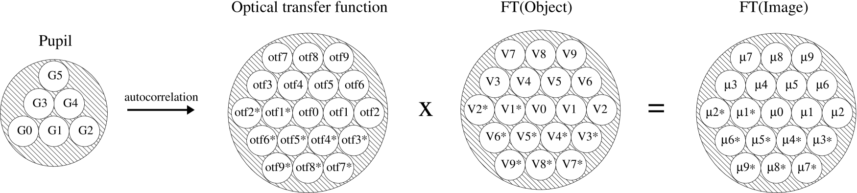
The image reconstruction problem is then reduced to finding the unknowns given the ’s. The ill-posedness of this task can be exhibited thanks to a simple example. In Fig. 1, the complex amplitude transmission in the pupil is binned into six different elements (the ’s). The autocorrelation of these six patches creates an OTF defined by a real value (at central spatial frequency) and 9 complex values . These OTF values multiplied by the visibility function of the astronomical object yield the Fourier transform of the observed image as one real value and 9 complex values . Since, by definition, the real value is equal to 1 and since the phase of one of the complex amplitude transmissions can be arbitrarily chosen, the image reconstruction involves the computation of 29 unknowns (15 complex values: , minus an arbitrary phase) given only 19 measurements (the real value and the 9 complex values ). Our example demonstrates that the image reconstruction when the PSF is unknown is an ill-posed problem termed as blind deconvolution (Thiébaut & Conan 1995). Without adding further information, disentangling astronomical from instrumental information is impossible.
To avoid having to disentangle the time-dependent OTF, a traditional solution is to average its fluctuations. Over multiple observations, the long exposure OTF is:
| (8) |
To calibrate the OTF, the astronomer can observe a point-like star (i.e. such that ) and apply the same averaging process. However, when phase variations become larger than wavelength, the average of the complex OTF tends toward 0, and deconvolution is impossible with a finite S/N ratio (Thiébaut 2005). In practice, long exposure images have a effective resolution, where in the visible is Fried’s parameter. Two solutions have been proposed to overcome this problem and achieve the diffraction limit at where is the pupil diameter. The first solution is to correct the wavefront in real time so as to keep the wavefront perturbations smaller than the wavelength. This is achieved with an adaptive optics system. The second solution, so called speckle interferometry (Labeyrie 1970), is to take short exposures with respect to the time scale of the perturbation, and to average the squared modulus of the Fourier transform of the image. This way, the transfer function for the modulus of the Fourier transform of the observed brightness distribution becomes:
| (9) |
and is attenuated for spatial frequencies higher than but different from zero up to . The Fourier phase of the observed brightness distribution can be retrieved by means of a third order technique such as the bispectrum (Weigelt 1977).
Here we propose an alternative approach. Instead of averaging the OTF, the goal is to have real time measurements of the complex amplitude transmission. Then, a post-detection algorithm can be used to obtain a calibrated OTF:
| (10) |
where and are estimated complex amplitude transmissions. We have however demonstrated in this section that this information is unavailable on a simple image of the object. In order to recover the missing information, we have proposed a system (Perrin et al. 2006), in which the telescope pupil is injected into an array of single-mode fibers, and rearranged into a new non-redundant exit pupil.
3 From an ill-posed to a well-posed problem
3.1 The instrument

The concept, proposed in Perrin et al. (2006), is summarised in Fig. 2. Briefly, entrance sub-apertures collect independently the radiation from an astronomical source in the pupil of the telescope, and focus the light onto the input heads of single-mode optical fibers (of location vectors ). The radiation is then guided by the fibers down to a recombination unit, in which the beams are rearranged into a 1D or 2D non-redundant configuration to form the exit pupil. Finally, the remapped output pupil is focused to form fringes in the focal plane where a different fringe pattern is obtained for every pair of sub-pupils.
The amplitudes and phases of the fringes are measurements of the Fourier components given by the entrance baselines vectors ; the Fourier components measured in the image are thus given by the relation:
| (11) |
where is the complex visibility of the observed object at the frequency , and and are the complex transmission factors in the telescope pupil as defined in Eq. (3). It is interesting to note the differences between this relation and Eq. (7): thanks to the remapping, each measurement now corresponds to a single pair of sub-apertures.
A second advantage of this setup comes from the fact that single-mode fibers act as spatial filters. As a consequence, the relation is exact for each sub-pupil. Indeed, after being filtered by the fiber, the complex electric field, which is otherwise a continuous function, can be characterized by only two parameters: its phase and its amplitude. The discretization introduced in the previous section is no longer an approximation which opens the way toward searching for an exact solution.
3.2 On the unicity of the solution
The fundamental idea of this paper comes from the fact that by using interferometric techniques, information can be retrieved to deconvolve an image from its PSF. As stated in Sect. 2, image restoration requires the knowledge of the complex transmission terms , which is impossible with direct imaging. However, Greenaway (1982) proved that the missing information can be encoded at higher frequencies (see also Arnot 1983; Arnot et al. 1985). Remapping enables an increase in the number of observables while keeping the number of unknowns constant. This is possible since the complex visibilities only depend on the baselines in the telescope entrance pupil. They do not change with a rearrangement of the pupil (Tallon & Tallon-Bosc 1992).
This can be well understood in terms of unknowns and observables. A remapped system is governed by Eq. (11). Providing sub-apertures and redundant entrance baselines, the number of complex unknowns are of visibilities ( terms), and transmission factors ( terms). On the other hand, the number of measurements is (the terms; with ). Hence, if , there are more observables than unknowns and the system of equations can be solved.
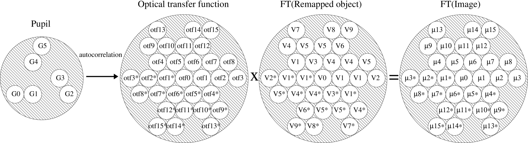
The fact that both the and the terms can be deduced from the can be illustrated in a specific case. Fig. 3 is the same sketch as in Fig. 1, but with the 6 sub-pupils rearranged into a non-redundant configuration. This configuration was chosen to have the most compact configuration, but any other non-redundant configuration could have been used (see for example Golay 1971). On the left panel are the complex transmission factors of the remapped pupil. The other panels show the Fourier transform values of, from left to right, the PSF, the astronomical object, and the image on the detector. The equation linking the observables to the unknowns and is Eq. (11). Inversion of the resulting set of equations may be possible since the number of unknowns is larger than the number of measurements. This can be demonstrated by using the logarithm of terms in Eq. (11), which becomes
| (12) |
for the real part, and
| (13) |
for the imaginary part. In these two equations, is the argument function, and , , and are as defined in Eq. (3). We obtain this way two sets of linear equations, one for for the phases:
| (14) |
and one for the amplitudes:
| (15) |
where represents column vectors. and are two matrices containing 1, 0, and -1 values. Specifically to the example of Fig. 3, Eq. (14) becomes:
The rank of this matrix is 12, while the number of unknowns is 15. The three terms of degeneracy are one for the absolute phase reference, and two for the tip and tilt. Thus, by providing an arbitrary constrain on these three terms (the absolute phase is arbitrary and the tip and tilt only depend on the location of the image centroid), we can perform a singular value decomposition of the matrix and obtain from the measurements a unique solution for the phase of the perturbations and object visibilities. The same method applies to the logarithm of the amplitude:
The rank of this matrix is 14, meaning all the amplitudes can be retrieved, except for the total brightness of the object. This parameter can easily be constrained by normalizing the flux of the reconstructed image. The measurement of the amplitudes is an important issue since we have to correct for injection variability in the single-mode fibers.
It is however clear that solving this system would require taking the logarithm of the measurements. This would be very sensitive to additive noise. To get the best out of the data, it is better to fit the measurements using their complex values and Eq. (11). To do so, we developed a self-calibration algorithm which permits the use of thousands of snapshot all together to reconstruct an image up to the photon noise limit.
3.3 A self-calibration algorithm for redundant arrays
This section presents a self-calibration algorithm adapted to single-mode pupil remapping instruments, but also more generally to any kind of redundant interferometric array. Indeed, the equation established in Sec 3.1 is common to all interferometric facilities. In the case of long baseline interferometry for example, is the measurement of the complex coherence value between telescopes and , the complex transmission factor of telescope , and the complex visibility of the astronomical object at the baseline formed by telescope and .
The particularity of this self-calibration algorithm comes from the fact that it gives complex visibility estimations without the need of a regularization term. This is possible thanks to the redundancy of the interferometric array. If one wants to make sure this algorithm is adapted to a specific interferometric facility, he would have first to establish the and matrices, and thus verify the unicity of the solution.
In the next sections, we first start deriving an algorithm in the single-exposure case (Sect. 3.3.1, 3.3.2 and 3.3.3), and then we show how to extend our algorithm to account for multiple exposures (Sect. 3.3.4, 3.3.5).
3.3.1 Log-likelihood
Following the Goodman (1985) model for the noise of measured complex visibilities, we assume that different measured complex visibilities are uncorrelated and that, for a given measured complex visibility , the real and imaginary parts are uncorrelated Gaussian random variables which have the same standard deviation. Under these assumptions and from Eq. (11), the log-likelihood of the data is:
| (16) |
where and are the complex transmissions for each sub-aperture and where is the set of sub-aperture pairs for which the interferences sample the -th spatial frequency as defined by Eq. (5). In Eq. (16), the statistical weights are:
| (17) |
Solving the image reconstruction problem, in the maximum likelihood sense, consists in seeking for the complex transmissions and the object visibilities which minimize the value of given by Eq. (16). Unfortunately, the log-likelihood being a polynomial of 6th degree with respect to the unknowns (the ’s and the ’s), proper means to minimize it have to be invented.
3.3.2 Best object visibilities
Given the complex transmissions , the expression of in Eq. (16) is quadratic with respect to the object complex visibilities . Providing the complex transmissions are known, obtaining the best object complex visibilities is then a simple linear least-squares problem. The solution of this problem is found by solving:
| (18) |
where, by linearity, the derivative of the real quantity with respect to the complex is defined as:
| (19) |
Then:
| (20) | |||||
Solving Eq. (18) with the partial derivative expression in Eq. (20) yields the best object visibilities given the data and the complex transmissions:
| (21) |
Not surprisingly, this solution is a weighted sum of the complex visibilities measured by sub-aperture pairs which sample the -th spatial frequency.
The visibilities obtained by Eq. (21) are not normalized. Assuming corresponds to the null frequency, the following normalization steps insure that the sought visibilities are normalized:
| (22) | ||||
| (23) | ||||
| (24) |
It is worth noting that the likelihood remains the same after these re-normalization steps.
3.3.3 Self-calibration stage
Since, given the complex transmission factors, the best object complex visibilities can be uniquely derived, the initial optimization problem of can be reduced to a smaller problem which consists in finding the complex transmissions which minimize the partially optimized log-likelihood:
| (25) |
where is given by Eq. (21), possibly after the re-normalization steps. The second stage of our algorithm therefore consists in fitting the complex transmissions so as to minimize with respect to the complex transmissions.
Since the criterion is continuously differentiable, its partial derivatives cancel at any extremum of the criterion. Hence the so-called first order optimality condition that at the optimum of we must have:
| (26) |
Note that, unless is strictly convex with respect to the ’s, Eq. (26) is a necessary condition but is not a sufficient one because it would be verified by all the extrema (local minima, local maxima or saddle points) of the criterion.
Since depends on , the chain rule must be applied to derive the partial derivative of with respect to the -th complex transmission. For instance, the derivative with respect to the real part of the -th complex transmission expands as:
However, since minimizes , we have:
and from the definition in Eq. (19) of the partial derivative with respect to a complex variable, we deduce that:
It follows that:
Since the same reasoning can be conducted for the derivative with respect to the imaginary part of the complex transmission and by definition of the derivation of a real quantity with respect to a complex variable given in Eq. (19), the partial derivative of the partially optimized log-likelihood finally simplifies to:
| (27) |
In words, since minimizes with respect to , the partial derivative of with respect to is simply the partial derivative of with respect to into which the is replaced (after derivation) by . This property helps to simplify the calculations to come and, more importantly, shows that the global optimum must verify the modified first order optimality condition:
| (28) |
Finally, the partial derivative of with respect to the complex transmissions can be written:
From this last expression, it is tempting to derive a simple iterative algorithm by solving Eq. (28) for assuming the other complex transmissions are known. The resulting recurrence equation is:
| (29) |
where is the -th complex transmission at -th iteration of the algorithm and is the -th best object visibility computed by Eq. (21) with the complex transmissions estimated at -th iteration:
| (30) |
3.3.4 Multiple exposure case
Our algorithm can be generalized to the processing of multiple exposures of the same object. We assume that the instrument does not undergo any significant rotation with respect to the observed object so that the sampled spatial frequencies (the ’s) and the corresponding sets of sub-aperture pairs (the ’s) remain the same during the total observing time. We also assume that the object brightness distribution is stable so that the object complex visibilities (the ’s) do not depend on the exposure time. At least because of the noise and of the turbulence, the measured complex visibilities and the instantaneous complex amplitude transmissions however do depend on the exposure index and are respectively denoted and . Under the Goodman (1985) approximation, the log-likelihood becomes:
| (31) |
where the, possibly time dependent, statistical weights are:
| (32) |
Since the object visibilities and the instrumental geometry do not depend on time, the same spatial frequency is measured at every exposure by a given pair of sub-apertures. Hence the condition given in Eq. (18) can be used to trivially obtain the best complex visibilities of the object:
| (33) |
which simplifies to Eq. (21) in the case of a single exposure.
3.3.5 Algorithm summary
Putting everything together, our algorithm consists in the following steps:
-
1.
initialization: set and choose the starting complex transmissions ;
-
2.
compute the best object visibilities given the complex transmissions according to Eq. (33) and, optionally, renormalize the unknowns;
-
3.
terminate if the algorithm converged; otherwise, proceed with next step;
-
4.
compute by updating the complex transmissions according to Eq. (34);
-
5.
let and loop to step 2;
Our iterative algorithm is very simple to implement and its modest memory requirements makes it possible to process over several thousands of snapshots all together. This is a requirement for faint objects or to achieve very high dynamic range. Yet, on a strict mathematical point of view, our algorithm may have a number of deficiencies. First, as already mentioned, the first order optimality condition is necessary but not sufficient to insure that the global minimum (or even a local minimum) of has been reached. Other non-linear image reconstruction algorithms (blind deconvolution, optical interferometry imaging, …) have the same restriction. In practice, checking that the algorithm converges toward a similar solution for different initial conditions can be used to assert the effective robustness of the method. A second possible problem results from the updating of the complex transmission by Eq. (34). If a fixed point is discovered by the recursion, then it satisfies the necessary optimality condition; but it is also possible that the recursion gives rise to oscillations for the values of the sought parameters. Note that our updating method is a non-linear one, analogous to numerical methods for solving linear equations such as the Jacobi and Gauss-Seidel methods (Barrett et al. 1994). Unlike for our specific problem, it is however possible to prove the convergence of the recursion in the linear case. Again, the behavior of the algorithm in practice can effectively prove its ability to converge to a fixed point. If it appears that the update formula leads to oscillations, this problem can be completely solved by using an iterative optimization algorithm which guarantees that the partially optimized log-likelihood is effectively reduced from one iteration to another. Since the log-likelihood is a sum of squares, a Levenberg-Marquardt algorithm (Moré 1977) coupled with a trust region method (Moré & Sorensen 1983) would completely solve this problem. In practice, none of the numerous simulations we have conducted with our iterative algorithm have given rise to any of these convergence problems.
Although derived in the specific case of a pupil remapping instrument, our algorithm shares similarities with the self-calibration method used in radio-astronomy (Cornwell & Wilkinson 1981). However, in our case, not only the phases of the complex transmissions are miscalibrated and must be recovered but also the amplitudes. Besides, we do not need a regularization term to overcome the sparsity of the coverage by radio interferometers. Our derivation of the non-linear updating formula in Eq. (34) is also quite similar to the iterative method proposed by Matson (1991) for recovering the Fourier phase from the bispectrum phase and later improved by Thiébaut (1994) to achieve better convergence capabilities.
4 Dynamic range estimations
4.1 Analytical estimation of the photon noise limitations
This system gives calibrated measurements of the spatial frequencies of the object. The advantage is straightforward. In classical imaging, phase and amplitude errors create speckles in the image plane, therefore limiting the dynamic range. With a pupil remapped instrument, and assuming we are acquiring fast enough to freeze atmospheric turbulence, statistical errors due to photon and detector noise will theoretically be the main limiting factor. Baldwin & Haniff (2002) showed that the dynamic range of a reconstructed image is linked to the errors of the Fourier components:
| (35) |
where is the total number of data points, is the fractional error in amplitude, and the phase error (in radians). For a total number of photons and a number of apertures , the amplitude of the fringe peaks in the Fourier transform of the image is equal to (assuming full coherence for the fringes). Considering a white photon noise of amplitude , the signal-to-noise of the visibility modulus can be estimated with
| (36) |
as for the phase (Goodman 1985):
| (37) |
This leads to the following approximation of the dynamic range:
| (38) |
Within these approximations, this result has the merit of clearly highlighting the advantage and the drawback of a single-mode remapping system: (i) an arbitrarily high dynamic range can be obtained anywhere in the image, providing the integration time is long enough; (ii) since additive noise is uniformly distributed on all the spatial frequencies, it is also evenly distributed across the whole field of view. To compare, an optical design isolating the photons of a bright object next to a faint companion – like a perfect adaptive optics and coronographic system – would achieve a superior photon-wise dynamic range of . Extreme dynamic range imaging, as required for detecting extra-solar earths (), would therefore also require a long integration time with our system.
4.2 Numerical simulations
4.2.1 Simulation setup
To perform these simulations, we used “YAO”, an adaptive optics simulation software written by F. Rigaut using the Yorick language. This software allows us to generate corrugated wavefront with and without adaptive optics correction. In our simulations, the instrumental setup corresponds to an 8 meter telescope under good seeing condition ( at ) caused by four different layers of turbulence at altitudes 0, 400, 6 000 and 9 000 meters. The wind speed ranges from 6 to depending on the altitude of the layer. The AO system is optimized to work in the near infrared. It consists in a classical Shack-Hartmann wavefront sensor and a actuator deformable mirror. The loop frequency has been set to , with a gain of 0.6 and a frame delay of 4 ms. The guide star is of magnitude 5.
The remapping was done by dividing the 8 meter telescope pupil into 132 hexagonal sub-pupils of 80 centimeters in diameter each. They are filtered by the fundamental mode of single-mode fibers, coupled so as to maximize the injection throughput of an uncorrupted incoming wavefront. The injection efficiency in this case would be of 78%. However, at the operating wavelength of , the diameters of the sub-pupils are large compare to the Fried parameter () and the coupling is expected to be much lower without adaptive optics ( in these simulations). The 132 sub-pupils are then rearranged in a non-redundant configuration, to produce a total of 8 646 sets of fringes on the detector.
The total integration time was set to 40 seconds. However, because of the coherence time of the atmosphere, acquisition was done by sequences of short acquisition periods. We used a snapshot time of 4 milliseconds, during which we integrated the effects of phase variations. This was a way to account for fringe blurring due to dynamic piston effects. We also added to our measurements the photon noise as a Gaussian noise of variance the number of photons on each pixel. The number of photons was computed to account for a coupling efficiency of 5% into the fibers and a spectral bandpass of .
No chromatic fringe blurring was introduced since its influence would highly depend on the chosen technical setup. Moreover, there are several ways to avoid this problem. In the case of a 1D non-redundant remapping, we recommend to spectrally disperse the fringes. If a 2D non-redundant reconfiguration is mandatory due to a large number of sub-pupils, another solution could be to use a hyper-chromatic magnifier like a Wynne lens system (as proposed by Ribak et al. 2004). At least, the use of a narrow spectral filter can completely avoid the chromatic blurring.
4.2.2 Comparison with the speckle and adaptive optics techniques
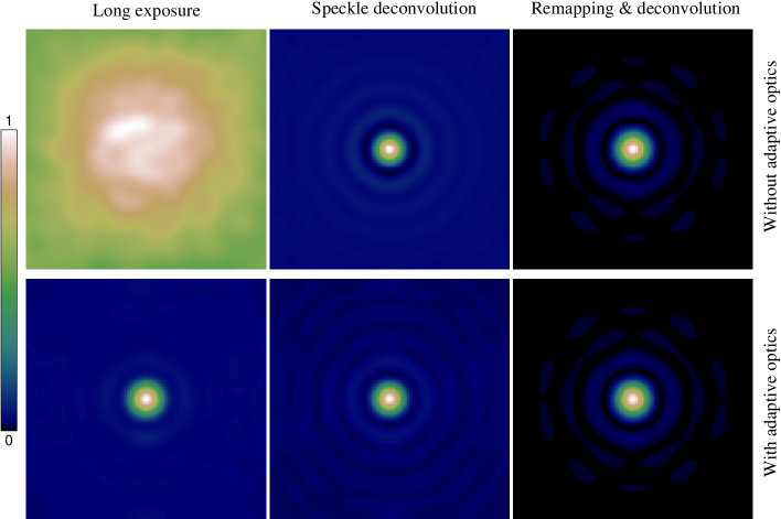
This first test was performed in order to demonstrate the reconstruction quality of the PSF. The astronomical object is a point-like source of Fourier transform values 1 (). The observing wavelength is 630 nm. As described in the previous section, the simulated dataset consists of 10 000 snapshots, each featuring 8646 fringe sets. From each set of fringes, a complex coherence value is extracted, and complex transmission factors are estimated according to the iterative algorithm described in Sect. 3.3.3. Finally, we used Eq. (10) to obtain the calibrated OTF, and thus the PSF. For comparison, the same corrugated wavefronts were used to obtain the PSF with two other techniques. The first one consists in averaging the complex instantaneous OTF by Eq. (8). The second one (speckle interferometry) consists in averaging the squared modulus, removing photon noise bias and taking the square root as in Eq. (9). In this work, we did not make use of the bispectrum or closure phase since our object is point-like and therefore purely symmetric. The four left panels of Fig. 5 represent the deduced PSF, with (lower panels) and without (upper panels) the use of an adaptive optics system.
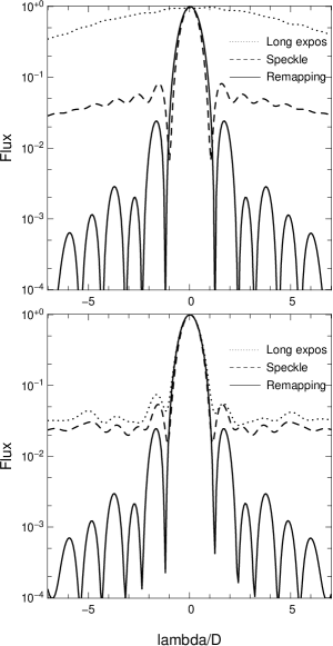
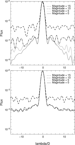
The first result confirm the usefulness of both speckle interferometry and adaptive optics systems, even though we are observing at visible wavelengths. This is clearly seen in Fig. 4; where unlike uncorrected long exposure imaging, they permit the retrieval of spatial information at the diffraction limit of the telescope. Nevertheless, the Strehl ratio in images obtained by these techniques is very low and the background pollution remains important. Without remapping, the best dynamic range achievable at visible wavelength is with a combination of AO and speckle interferometry technique, which provide a dynamic range of 40. This of course is in the case of a perfectly working near-infrared AO system with a 500 Hz frequency loop. Most current AO system are not used in that mode since any slight miss-calibration of the actuator influence function would make it useless at these wavelengths.
On the other hand, a diffraction pattern is obtained by using our remapping instrument and our image reconstruction algorithm. The pattern differs slightly from a perfect Airy disc due to the hexagonal sampling of the OTF. At a few from the central star, a dynamic range of is obtained (see Fig. 4). Using an adaptive optics system does not significantly modify the pattern, meaning that the dynamic range is limited by the shape of the perturbation free PSF. Our conclusion is therefore that the dynamic range could be further increased by choosing a different PSF. We did this in the following section over a complex astronomical object.
4.2.3 Image reconstruction
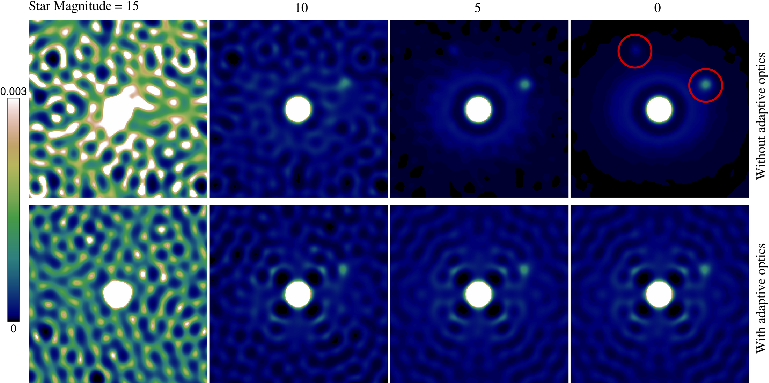
In this simulation, the astronomical object is a star surrounded by a protoplanetary disc. The disc has an exponential brightness distribution and a total flux of a hundredth of the star flux. Two companions are also present, one with a flux of a thousandth, and the other of ten thousandths the flux of the star.
As before, the complex transmissions are estimated by using iteratively Eq. (29). But unlike in Sect. 4.2.2, calibrated object visibilities are retrieved by our algorithm using Eq. (33) from 10 000 short exposure images. We used these visibilities to reconstruct an image. But instead of doing a simple Fourier transform to obtain the equivalent of a dirty map, it is possible to choose the PSF according to a scientific goal. For example, an Airy disc PSF is good to achieve high angular resolution, while a Gaussian apodization is better for the dynamic range. Of course, any other visibility apodization can also be applied to obtain the most suitable PSF. This system thus has the advantage of producing images close to what can be obtained with optically apodized pupil optics (Kuchner & Traub 2002; Guyon 2003), while completely free of any atmospheric perturbations. This way, the dynamic range is no longer limited by the Airy rings of the diffraction pattern of the telescope.
However, there is one perturbation this system cannot correct for; it is the photon noise. The phase corrugation being accounted for, the photon noise should be the theoretical limit of the dynamic range. To try to reach this limit, we used a Gaussian shape apodization on the visibilities. All of the image reconstructions in Fig. 6 are of the object described in the first paragraph of this section, but with different total brightnesses. The reconstructions from the left to the right are respectively of a central star of magnitude 15, 10, 5, and 0. The upper set of panels are for a system without AO, while the four bottom panels are with AO activated. Fig. 7 gives a summary by plotting a horizontal cut of the different reconstructions. Table 1 lists the dynamic ranges estimated on the images and compares them with the analytical approximation of the photon noise established in Sect. 4.1. The dynamic range estimations are obtained by taking the inverse of the root mean square of the background of the image normalized by its pixel of maximum flux.
When atmospheric turbulence is not corrected by an AO system, the reconstructions clearly highlights a dynamic range limited by photon noise. For an object of magnitude 10, we achieved a dynamic range of . This is comparable to what was calculated from the total photon count and the analytical relation . This theoretical value, taking into account the 5% coupling efficiency in the fibers, was of . A second interesting point is that when the brightness of the source increases by a factor 100 (delta mag = 5), the dynamic range increases by a factor around 10. This can be seen over 15 order of magnitude, indicating that the dynamic range has a roughly linear increase as a function of . This does 1) confirm the validity of the analytical estimation, and 2) prove the quality of our self calibration algorithm to restore the object visibilities.
Noteworthy is the reconstruction of the system with a brightness of 15 mag. Due to a relatively low coupling efficiency in the fibers, an average of 250 photons are detected per 4 ms snapshot. According to Eq. (36), it implies a S/N ratio of for each spatial frequency measurement. It is therefore impressive to note that even with such a vague knowledge of the , the iterative algorithm of Sect. 3.3.3 is capable of restoring images with a dynamic range limited by the photon noise. This is possible since it combines the advantage of fitting the information from all snapshots together with a small, cpu friendly, recursive algorithm.
When atmospheric turbulence is corrected by an AO system, the dynamic range does not increase linearly as a function of the brightness anymore. Indeed, in the lower panels of Fig. 6 and Fig. 7, the dynamic range is clearly limited by another factor. Thanks to the correction, the injection throughput is higher, around 23%. This allows an increase in dynamic range for the faintest source, but with a saturation around a few . The reason for this unpredicted threshold appeared clearly when analyzing our simulations. During the 4 ms integration time, mirror displacements happened twice to adapt for the atmospheric turbulence. These minor corrections, while increasing the spatial coherence (Cagigal & Canales 2000), have the drawback of introducing a phase noise overshoot at the frequency of the loop. This side effect results in a slight blurring of the fringes recorded on the detector and a bias on the measurements. To profit from the advantages of the AO, solutions could either be to increase the acquisition rate, or, better, to adjust the control loop to decrease the amplitude of the overshoot.
{
5 Summary
In this paper, we presented further investigation of the instrument introduced in Perrin et al. (2006).
- •
-
•
We developed an analytical iterative self-calibration algorithm which enables inversion of the previously established equation over several thousands of snapshots simultaneously. This algorithm happened to be robust, allowing visibility determination from Fourier component measurements with S/N ratio well below 1 (Sect. 3.3).
-
•
Simulations of this system confirmed the validity of the algorithm and produced high dynamic range, diffraction limited, images of complex astronomical objects. A dynamic range of the order of was achieved at visible wavelength on an eight meter telescope and in the presence of good seeing conditions. Compared to actual AO systems, it represents an increase of around in dynamic range. We noted that the sensitivity of the instrument would increase by using an adaptive optics system, but at the price of a limitation in the achievable dynamic range (Sect. 4).
Acknowledgments
The authors would like to thank F. Rigaut for letting “YAO” freely available to the astronomical community. “YAO” is a simulation tool for adaptive optics systems, available on the web site http://www.maumae.net/yao/. Simulations and data processing for this work have been done using Yorick language which is freely available at http://yorick.sourceforge.net/. The authors would also like to thank the many people with whom discussing helped a lot to mature this paper. These persons include F. Assemat, P. Baudoz, A. Bocalletti, V. Coudé du Foresto, E. Ribak, G. Rousset and P. Tuthill.
References
- Arnot (1983) Arnot N. R., 1983, Optics Communications, 45, 380
- Arnot et al. (1985) Arnot N. R., Atherton P. D., Greenaway A. H., Noordam J. E., 1985, Traitement du Signal, 2, 129
- Baldwin & Haniff (2002) Baldwin J. E., Haniff C. A., 2002, Phil. Trans. R. Soc. London, 360, 969
- Barrett et al. (1994) Barrett R., Berry M., Chan T. F., Demmel J., Donato J., Dongarra J., Eijkhout V., Pozo R., Romine C., der Vorst H. V., 1994, Templates for the Solution of Linear Systems: Building Blocks for Iterative Methods. SIAM, Philadelphia, PA
- Cagigal & Canales (2000) Cagigal M. P., Canales V. F., 2000, Optical Society of America Journal A, 17, 903
- Cornwell & Wilkinson (1981) Cornwell T. J., Wilkinson P. N., 1981, MNRAS, 196, 1067
- Golay (1971) Golay M. J. E., 1971, J. Opt. Soc. Am., 61, 272
- Goodman (1985) Goodman J. W., 1985, Satistical Optics. John Wiley & Sons
- Greenaway (1982) Greenaway A. H., 1982, Optics Communications, 42, 157
- Guyon (2003) Guyon O., 2003, A&A, 404, 379
- Haniff et al. (1987) Haniff C. A., Mackay C. D., Titterington D. J., Sivia D., Baldwin J. E., 1987, Nature, 328, 694
- Kuchner & Traub (2002) Kuchner M. J., Traub W. A., 2002, ApJ, 570, 900
- Labeyrie (1970) Labeyrie A., 1970, A&A, 6, 85
- Matson (1991) Matson C. L., 1991, J. Opt. Soc. Am. A, 8, 1905
- Moré (1977) Moré J. J., 1977, in Watson G. A., ed., Lecture Notes in Mathematics, Vol. 630, Numerical Analysis. Springer-Verlag
- Moré & Sorensen (1983) Moré J. J., Sorensen D. C., 1983, SIAM J. Sci. Stat. Comp., 4, 553
- Perrin et al. (2006) Perrin G., Lacour S., Woillez J., Thiebaut E., 2006, ArXiv Astrophysics e-prints
- Ribak et al. (2004) Ribak E. N., Perrin G. S., Lacour S., 2004, in Traub W. A., ed., New Frontiers in Stellar Interferometry, Proceedings of SPIE Volume 5491. Edited by Wesley A. Traub. Bellingham, WA: The International Society for Optical Engineering, 2004., p.1624 Multiple-beam combination for faint objects. pp 1624–+
- Tallon & Tallon-Bosc (1992) Tallon M., Tallon-Bosc I., 1992, A&A, 253, 641
- Thiébaut (1994) Thiébaut E., 1994, PhD thesis, Université de Paris 7
- Thiébaut (2005) Thiébaut E., 2005, in Foy R., Foy F.-C., eds, NATO ASI, Optics in Astrophysics. Kluwer Academic
- Thiébaut & Conan (1995) Thiébaut E., Conan J.-M., 1995, J. Opt. Soc. Am. A, 12, 485
- Tuthill et al. (2000) Tuthill P. G., Monnier J. D., Danchi W. C., Wishnow E. H., Haniff C. A., 2000, PASP, 112, 555
- Weigelt (1977) Weigelt G., 1977, Opt. Commun., 21, 55