Three-dimensional hydrodynamic simulations of asymmetric pulsar wind bow shocks

Abstract

We present three-dimensional, nonrelativistic, hydrodynamic simulations of bow shocks in pulsar wind nebulae. The simulations are performed for a range of initial and boundary conditions to quantify the degree of asymmetry produced by latitudinal variations in the momentum flux of the pulsar wind, radiative cooling in the postshock flow, and density gradients in the interstellar medium (ISM). We find that the bow shock is stable even when travelling through a strong ISM gradient. We demonstrate how the shape of the bow shock changes when the pulsar encounters density variations in the ISM. We show that a density wall can account for the peculiar bow shock shapes of the nebulae around PSR J2124-3358 and PSR B0740-28. A wall produces kinks in the shock, whereas a smooth ISM density gradient tilts the shock. We conclude that the anisotropy of the wind momentum flux alone cannot explain the observed bow shock morphologies but it is instead necessary to take into account external effects. We show that the analytic (single layer, thin shell) solution is a good approximation when the momentum flux is anisotropic, fails for a steep ISM density gradient, and approaches the numerical solution for efficient cooling. We provide analytic expressions for the latitudinal dependence of a vacuum-dipole wind and the associated shock shape, and compare the results to a split-monopole wind. We find that we are unable to distinguish between these two wind models purely from the bow shock morphology.

1 Introduction

After a pulsar escapes its supernova remnant, it typically travels supersonically through the interstellar medium (ISM), sometimes with speeds in excess of 1000 km s^-1 (Chatterjee et al., 2005). At the same time, pulsars emit highly relativistic winds, probably consisting of electron-positron pairs, with bulk Lorentz factor between $10^{2}$ and $10^{6}$ (Kennel & Coroniti, 1984a; Spitkovsky & Arons, 2004). The interaction of the pulsar wind with the ISM produces a characteristic multilayer shock structure (Bucciantini, 2002; van der Swaluw et al., 2003).

The multilayer structure of pulsar wind nebulae (PWN) gives rise to a variety of observable features at different wavelengths; see Gaensler & Slane (2006) for a recent review. The outer bow shock excites neutral hydrogen atoms either collisionally or by charge exchange, which then de-excite and emit optical H$\alpha$ radiation (Bucciantini & Bandiera, 2001). The microphysics of these excitation processes was treated in the context of supernova remnants by Chevalier & Raymond (1978) and Chevalier et al. (1980), while Ghavamian et al. (2001) performed detailed calculations of the ionization structure and optical spectra produced by non-radiative supernova remnants in partially neutral gas. Presently, six PWN have been detected in the optical band (Gaensler & Slane, 2006; Kaspi et al., 2004), namely around the pulsars PSR B1957+20 (Kulkarni & Hester, 1988), PSR B2224+65 (Cordes et al., 1993), also called the Guitar Nebula, PSR B0740$-$28 (Jones et al., 2002), PSR J0437$-$4715 (Bell et al., 1995), RX J1856.5$-$3754 (van Kerkwijk & Kulkarni, 2001), and PSR J2124$-$3358 (Gaensler et al., 2002).

Pulsar bow shocks directly probe the conditions in the local ISM. The size of the bow shock scales with the standoff distance (Chatterjee & Cordes, 2002; Wilkin, 1996), defined as the point where the ISM ram pressure balances the wind ram pressure. As the wind ram pressure is given directly by the (measurable) spin-down luminosity of the pulsar for both young pulsars (Kennel & Coroniti, 1984a) and recycled millisecond pulsars (Stappers et al., 2003), the size of the bow shock can put an upper limit on the ISM density, given a measurement of the pulsar’s proper motion. Furthermore, the morphology of the shock gives detailed information about the inhomogeneity of the ISM. Density gradients have been proposed to explain the peculiar shapes of the bow shocks around the pulsars PSR B0740$-$28 (Jones et al., 2002) and PSR J2124$-$3358 (Gaensler et al., 2002). Chatterjee et al. (2006) recently showed that the kink in the PWN around PSR J2124$-$3358 can be explained if the pulsar is travelling through a density discontinuity in the ISM (a “wall”).

Our theoretical understanding of the wind acceleration mechanism, in particular the angular distribution of its momentum flux, is still incomplete. Goldreich & Julian (1969) showed that a pulsar has an extended magnetosphere filled with charged particles that are accelerated into a surrounding wave zone (Coroniti, 1990). Although the nature of the energy transport in the pulsar wind is still an unsolved question, probably governed by non-ideal magnetohydrodynamics (Melatos & Melrose, 1996), all models agree that it is dominated by the Poynting flux near the star. However, observations of the Crab nebula (Kennel & Coroniti, 1984a) and PSR B1509$-$58 (Gaensler et al., 2002) imply a value for the magnetisation parameter, $\sigma$, defined as the ratio of the Poynting flux to the kinetic energy flux, satisfying $\sigma<0.01$ at the wind termination shock. In other words, a transition from high $\sigma$ to low $\sigma$ must occur between the magnetosphere and the termination shock, a problem commonly referred to as the $\sigma$ paradox. While it is generally assumed that the angular dependence of the momentum flux is preserved during this transition (Del Zanna et al., 2004), the exact dependence is unknown. The split-monopole model predicts a mainly equatorial flux (Bogovalov, 1999; Bucciantini, 2006) while wave-like dipole models (Melatos & Melrose, 1996) predict a more complicated distribution. The study of the termination shock structure, including its variability (Spitkovsky & Arons, 2004; Melatos et al., 2005), thus provides valuable information about the angular distribution of the wind momentum flux and hence the electrodynamics of the pulsar magnetosphere.

PWN also emit synchrotron radiation at radio and X-ray wavelengths (Gaensler & Slane, 2006; Kaspi et al., 2004) from wind particles which are accelerated in the inner shock and subsequently gyrate in the nebular magnetic field (Kennel & Coroniti, 1984b; Spitkovsky & Arons, 1999). If the pulsar moves supersonically, the (termination) shock is strongly confined by the ISM ram pressure (Bucciantini, 2002; van der Swaluw et al., 2003) and elongates opposite the direction of motion. X-ray-emitting particles with short synchrotron lifetimes directly probe the inner flow structure of the PWN. With the help of combined X-ray and radio observations, Gaensler et al. (2004) identified the termination shock and post shock flow in the PWN around PSR J1747$-$2958, the Mouse Nebula. They found that the data are consistent with an isotropic momentum flux distribution, a statement that holds for some other bow shocks, e.g. PSR B2224$-$65 (Chatterjee & Cordes, 2002), but not all, e.g. IC433 (Gaensler & Slane, 2006).

Before we can use PWN to probe the ISM, a precise knowledge of the inner flow structure and the response of the system to external influences is important. Although Wilkin (1996) found an analytic solution for the shape of the bow shock in the limit of a thin shock, the complexity of the problem generally requires a numerical treatment. Bucciantini (2002) performed hydrodynamic, 2.5-dimensional, cylindrically symmetric simulations to explore the validity of a two-shell approximation to the problem and elucidated the inner, multilayer shock structure. van der Swaluw et al. (2003) modelled a pulsar passing through its own supernova remnant and found that the bow shock nebula remains undisrupted.

Of course, the validity of a hydrodynamic approach is limited. To compute synchrotron maps, magnetic fields must be included. Relativistic magnetohydrodynamic (RMHD) simulations by Komissarov & Lyubarsky (2003, 2004) explain the peculiar jet-like emission in the Crab nebula by magnetic collimation of the back flow of an anisotropic pulsar wind, a result confirmed later by Del Zanna et al. (2004). RMHD simulations of bow shocks around fast moving pulsars by Bucciantini et al. (2005) and Bogovalov et al. (2005) assume cylindrical symmetry and an isotropic pulsar wind.

The chief new contribution of this paper is to relax the assumption of cylindrical symmetry. We perform fully three-dimensional, hydrodynamic simulations of PWN, focusing on observable features which can be compared directly to observations. Although pulsar winds are generally expected to be symmetric around the pulsar rotation axis (even if the momentum flux varies strongly with latitude), there are external factors, like an ISM density gradient, which destroy the cylindrical symmetry. The existence of two very different speeds, namely that of the relativistic wind and the pulsar proper motion, presents a significant numerical challenge in three dimensions, which we overcome by using a parallelised hydrodynamic code, with adaptive-mesh Godunov-type shock-capturing capabilities.

After describing the numerical method in section 2, we present the results of our simulations for different types of asymmetry, namely anisotropic momentum flux (section 3), the effects of uniform cooling (section 4), an ISM density gradient (section 5), and an ISM barrier or “wall” (section 6). We conclude by discussing what information can be deduced about the ISM and the pulsar wind when the results are combined with observations in section 7.

2 Numerical Method

2.1 Hydrodynamic model

The simulations are performed using Flash (Fryxell et al., 2000), a parallelized hydrodynamic solver based on the second-order piecewise parabolic method (PPM). Flash solves the inviscid hydrodynamic equations in conservative form,

$$0 = \frac{\partial\rho}{\partial t}+\nabla\cdot\left(\rho\mn@boldsymbol{v}\right),$$ (1)

$$0 = \frac{\partial(\rho\mn@boldsymbol{v})}{\partial t}+\nabla\cdot\left(\rho\mn@boldsymbol{v}\mn@boldsymbol{v}\right)+\nabla P,$$ (2)

$$0 = \frac{\partial(\rho E)}{\partial t}+\nabla\cdot\left[\left(\rho E+P\right)\mn@boldsymbol{v}\right],$$ (3)

together with an ideal gas equation of state,

$$P=\left(\gamma-1\right)\rho\epsilon,$$ (4)

where $\rho$, $P$, $\epsilon$ and $\mn@boldsymbol{v}$ denote the density, pressure, internal energy per unit mass, and velocity, respectively, and $E=\epsilon+|\mn@boldsymbol{v}|^{2}/2$ is the total energy per unit mass. We take advantage of the multifluid capability of Flash to treat the pulsar wind and the interstellar medium as fluids with different adiabatic indices $\gamma_{1}$ and $\gamma_{2}$, respectively. The weighted average adiabatic index $\gamma$ can then be computed from

$$\frac{1}{\gamma-1}=\frac{X_{1}}{\gamma_{1}-1}+\frac{X_{2}}{\gamma_{2}-1},$$ (5)

where $X_{i}$ is the mass fraction of each fluid, advected according to

$$\frac{\partial(\rho X_{i})}{\partial t}+\nabla\cdot\left(\rho X_{i}\mn@boldsymbol{v}\right)=0.$$ (6)

We do not consider reactive flows, so there is only a small amount of numerical mixing between the two fluids. For the problem studied here, we find empirically that the results are qualitatively the same for $\gamma_{1}=\gamma_{2}$ and $\gamma_{1}\neq\gamma_{2}$ (see section 3.2) and therefore take $\gamma_{1}=\gamma_{2}=5/3$ in most of our simulations, using the multifluid capability only to trace the contact discontinuity.

Flash manages the adaptive mesh with the Paramesh library (Olson et al., 1999). The mesh is refined and coarsened in response to the second-order error in the dynamical variables (for details, see Loehner, 1987). We perform our simulations on a three-dimensional Cartesian grid with $8\times 8\times 8$ cells per block and a maximum refinement level of five nested blocks, giving a maximum resolution of $128^{3}$ cells.

We are limited by processing capacity to simulations lasting $\sim 15\tau_{0}$, where $\tau_{0}$ is the time for the ISM to cross the integration volume. Unfortunately, this is not always sufficient to reach a genuine steady state. We occasionally encounter ripples in the shock [e.g. Figure 3 (right), discussed further in section 3] which are numerical artifacts which diminish as the simulation progresses.

2.2 Boundary and initial conditions

The simulations are performed in the pulsar rest frame. Figure 1 depicts the pulsar and the orientation of its rotation axis $\mathbf{\Omega}$ with respect to the velocity vector $\mathbf{v}_{m}$ of the ISM in this frame. The momentum flux of the pulsar wind is assumed to be cylindrically symmetric about $\mathbf{\Omega}$, in keeping with simplified theoretical models like the split monopole (Bogovalov, 1999; Komissarov & Lyubarsky, 2003) or vacuum dipole (Melatos & Melrose, 1996; Melatos, 1997, 2002).

In the pulsar’s rest frame, the ISM appears as a steady wind that enters the integration volume from the upper boundary $z=z_{\mathrm{max}}$, with velocity $\mathbf{v}_{m}=-\mathbf{v}_{p}=-4\times 10^{7}$ cm s${}^{-1}\,\mn@boldsymbol{\hat{z}}$, where $\mathbf{v}_{p}$ is the pulsar’s velocity in the observer’s frame (Hobbs et al., 2005), density $\rho_{m}=($0.33–1.30$)\times 10^{-23}$ g cm^-3, and specific internal energy $\epsilon_{m}=1.18\times 10^{12}$ erg g^-1. The sound speed $c_{m}=1.15\times 10^{6}$ cm s^-1 and Mach number $M_{m}=v_{m}/c_{m}=35$ are typical of the parameters inferred for a variety of observed PWN (Kaspi et al., 2004; Bucciantini et al., 2005). All boundaries except $z=z_{\mathrm{max}}$ act as outflow boundaries, where the values of all the dynamical variables are equalized in the boundary cells and integration region (zero gradient condition). These boundary conditions are justified provided that the flow speed across the boundaries exceeds the sound speed thus preventing a casual connection of the regions inside and outside the computational domain. We check this assumption a posteriori in section 3.2. Initially, we set $\rho=\rho_{m}$, $\mathbf{v}=(0,0,-v_{m})$, and $\epsilon=\epsilon_{m}$ in every cell.

We allow for the possibility that the pulsar travels into a density gradient. This may be either a smooth gradient perpendicular to the pulsar’s direction of motion (section 5) or an extended ridge of high density material making an angle $\alpha$ with $\mathbf{v}_{m}$, which we call a “wall”, also depicted in figure 1 (section 6). The boundary conditions corresponding to these scenarios are defined in section 5 and 6.

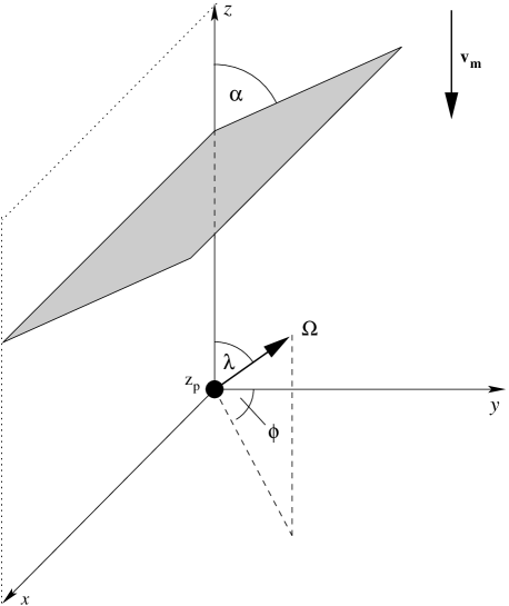
Figure 1: Orientation of the pulsar, wall, and Cartesian coordinate axes in the pulsar’s rest frame. The pulsar is located at $(0,0,z_{p}$) and the interstellar medium moves parallel to the $z$ axis with a speed $v_{m}$. The symmetry axis $\mathbf{\Omega}$ of the wind (assumed to be the pulsar’s rotation axis) is defined by its polar angle $\lambda$ and azimuthal angle $\phi$. The wall lies perpendicular to the $y$-$z$ plane, making an angle $\alpha$ with respect to the $z$ axis.

The simulation parameters for the different models are listed in table 1.

3 Anisotropic wind

Although the electrodynamics of pulsar wind acceleration and collimation remains unsolved, observations of PWN (Helfand et al., 2001; Gaensler et al., 2002; Roberts et al., 2003) as well as theoretical studies of split-monopole (Bogovalov, 1999; Komissarov & Lyubarsky, 2003, 2004) and wave-like dipole (Melatos & Melrose, 1996; Melatos, 1997, 2002) outflows seem to favor anisotropic momentum and energy flux distributions, where the wind is cylindrically symmetric about $\mathbf{\Omega}$ but varies in strength as a function of latitude. Letting $\theta$ denote the colatitude measured relative to $\mathbf{\Omega}$, the various models predict the following momentum flux distributions: $g_{w}(\theta)=\sin^{2}\theta+1/\sigma$ for the split monopole (Bogovalov, 1999; Komissarov & Lyubarsky, 2003; Arons, 2004), $g_{w}(\theta)=\cos^{2}\theta+1$ for the point dipole, and $g_{w}(\theta)=2\cos^{4}\theta+6\cos^{2}\theta+5$ for the extended dipole (Melatos 1997; see also appendix A). The normalized momentum flux $g_{w}(\theta)$ is defined precisely in appendix B.

3.1 Numerical implementation

We implement the wind anisotropy by varying the wind density $\rho_{w}$ according to

$$\rho_{w}(\theta)=\rho_{0,w}g_{w}(\theta)=\rho_{0,w}\left(c_{0}+c_{2}\cos^{p}\theta\right),$$ (7)

where $c_{0}$, $c_{2}$ and $p$ are constants, while leaving the wind velocity $\mathbf{v}_{w}$ constant. Strictly speaking, this is unrealistic, because it is likely that $\mathbf{v}_{w}$ varies with $\theta$ too in a true pulsar wind. However, it is expected to be an excellent approximation because Wilkin (1996, 2000) showed that the shape of the bow shock is a function of the momentum flux $\rho_{w}v_{w}^{2}$ only, not $\rho_{w}$ and $\mathbf{v_{w}}$ separately, at least in the thin-shell limit of a radiative shock. We deliberately choose equation (7) to have exactly the same form as in the analytic theory (Wilkin, 1996, 2000) to assist comparison below.

In equation (7), $c_{0}$ and $c_{2}$ parametrize the anisotropy of the wind, while $p$ can be used to model jet-like outflows (e.g. $p\geq 4$). For $p=2$, equation (7) is equivalent to equation (109) of Wilkin (2000). The split-monopole model corresponds to $p=2$ and $c_{2}=-1$ (Komissarov & Lyubarsky, 2003). Note that normalisation requires $c_{0}=1-c_{2}/3$ for $p=2$ and $c_{0}=1-c_{2}/5$ for $p=4$. The analytic solutions for these two cases are presented in appendix A.

Although the pulsar wind is ultrarelativistic [e.g. Lorentz factor $10^{2}-10^{6}$ in the Crab Nebula; Kennel & Coroniti (1984a); Spitkovsky & Arons (2004)], the shape is determined by the ratio of the momentum fluxes alone (Wilkin, 1996, 2000). We can therefore expect our model to accurately describe the flow structure, as long as the value of the mean flux $\rho_{0,w}v_{w}^{2}=4.6\times 10^{-8}$ g cm^-1 s^-2 is realistic (which it is), even though we have $v_{w}\ll c$. This approach was also adopted by Bucciantini (2002) and van der Swaluw et al. (2003). Bucciantini et al. (2005) performed RMHD simulations of PWN and a comparison of our results with theirs does not reveal any specifically relativistic effects; RMHD simulations with low $\sigma$ agree qualitatively with non-relativistic hydrodynamical simulations. In other words, as long as we choose $\rho_{w}$ and $\mathbf{v}_{w}$ such that $\rho_{w}v_{w}^{2}=\dot{E}/4\pi r_{w}^{2}c$, where $\dot{E}$ is the pulsar’s spin-down luminosity (and $r_{w}$ is defined in the next paragraph), we get the same final result.

The pulsar wind has density $\rho_{0,w}=4.6\times 10^{-24}$ g cm^-3, specific internal energy $\epsilon_{w}=5.9\times 10^{12}$ erg g^-1, and velocity $\mn@boldsymbol{v}_{w}=v_{w}\mn@boldsymbol{e}_{r}$, where $\mn@boldsymbol{e}_{r}$ is the radial unit vector and $v_{w}=10^{8}$ cm s^-1. This particular choice gives a sound speed $c_{w}=2.5\times 10^{6}$ cm s^-1 and Mach number $M_{w}=40$. The pulsar wind is launched by restoring the dynamical variables $\rho_{w},\mathbf{v}_{w}$ and $\epsilon_{w}$ in a spherical region with radius $r_{w}=6.2\times 10^{15}$ cm around $\mn@boldsymbol{r}_{p}=(0,0,z_{p})$ (figure 1) to their initial values after every timestep.

Table 1: Model parameters. The wind momentum flux is proportional to $1-c_{2}/3+c_{2}\cos^{p}\theta$, where $\theta$ is the colatitude measured with respect to the pulsar spin axis $\mathbf{\Omega}$, and $\lambda$ and $\phi$ define the orientation of this axis (figure 1 and section 3). $R_{0}$ is the standoff distance as measured from the simulation output, $f$ stands for the cooling efficiency (section 4), and $H$ is the scale-height of the ambient density gradient (section 5). The wall (section 6) is described by the density contrast $\eta=\rho_{w}/\rho_{m}$, the angle $\alpha$, and the distance over which the density rises ($\Delta_{r}$) and declines ($\Delta_{d}$). The dots indicate parameters that are not used in that simulation.

Model	$p$	$c_{2}$	$\lambda$ [°]	$\phi$ [°]	$R_{0}$ [cm/$10^{16}$]	$\log f$	$H/R_{0}$	$\rho_{m}$ [g cm${}^{-3}/10^{-23}$]	$\eta$	$\alpha$ [°]	$\Delta_{r}/R_{0}$	$\Delta_{d}/R_{0}$
A	2	3	45	0	1.5	…	…	1.30	…	…	…
B	2	3	90	0	1.5	…	…	1.30	…	…	…	…
C	4	3	45	0	2	…	…	1.30	…	…	…
A1	2	–1	45	0	2.2	…	…	1.30	…	…	…
C1	2	3	35	0	2	$-4$	…	1.30	…	…	…	…
C2	2	3	35	0	2	$-3$	…	1.30	…	…	…	…
C3	2	3	35	0	1.8	$-2$	…	1.30	…	…	…	…
C4	2	3	35	0	1.8	$0$	…	1.30	…	…	…	…
D	…	…	…	…	1.85	…	1.5	1.30	…	…	…	…
E	…	…	…	…	1.85	…	1.0	1.30	…	…	…	…
F	…	…	…	…	1.85	…	0.5	1.30	…	…	…	…
G	…	…	…	…	1.85	…	0.25	1.30	…	…	…	…
W1	4	1	90	45	2	…	…	0.52	2.5	26.6	0.5	…
SA	4	1	90	–45	2	…	…	0.33	4	26.6	0.5	25
SB	4	1	90	–45	2	…	…	0.33	4	63.4	0.5	25

3.2 Multilayer shock structure

Figure 2 shows the $y$-$z$ section of model A, a typical anisotropic wind with $p=2$ and $c_{2}=3$ in which $\mathbf{\Omega}$ is tilted by $45$°with respect to $\mathbf{v}_{p}$. This wind is pole-dominated, with zero momentum flux at the equator, contrary to what is inferred from observation (Gaensler & Slane, 2006). We postpone a detailed comparison between a pole-dominated and an equatorially-dominated outflow to section 3.4 and discuss here only the shock structure, which is common to both cases.

All our simulations show the characteristic multilayer structure in figure 2, described also by van der Swaluw et al. (2003) and Bucciantini (2002). The pulsar wind inflates a wind cavity that is enclosed by a termination shock (TS). The location of the TS behind the pulsar is determined by the thermal pressure in the ISM (Bucciantini, 2002; van der Swaluw et al., 2003). Ahead of the pulsar, the termination shock is confined by the ram pressure of the ISM. The wind material is thermalised at the TS and fills a cylindrical postshock region (PS), separated from the shocked ISM by a contact discontinuity (CD).

In the case of a thin shock, the shape of the CD can be described analytically (Wilkin, 2000, see also appendix A), with a global length scale $R_{0}$ which is computed by equating the ram pressures of the ISM and the wind:

$$R_{0}=\left(\frac{\dot{E}}{4\pi\rho_{m}v_{m}^{2}v_{w}}\right)^{1/2}.$$ (8)

The analytic solution is depicted by a solid curve (scaled to match the CD) and by a dotted curve (scaled to match the BS) in figure 2. As discussed below (section 3.3), it describes the location of the CD and the BS, respectively, reasonably well.

For an isotropic wind, $R_{0}$ equals the standoff distance, defined as the distance from the pulsar to the intersection point of the pulsar’s velocity vector and the bow shock apex. For an anisotropic wind, however, the standoff distance also depends on the exact distribution of momentum flux and $R_{0}$ is merely an overall length-scale parameter (Wilkin, 2000).

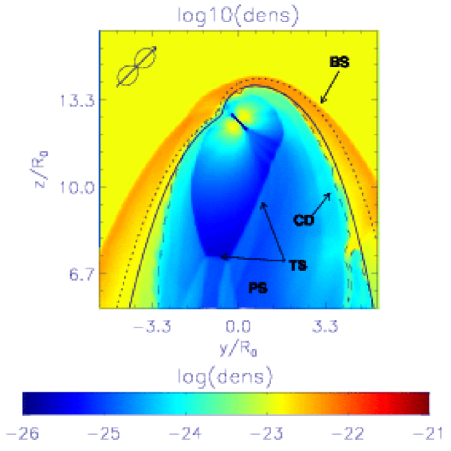
Figure 2: $y$-$z$ section of model A. The colors denote the density in logarithmic scale, as indicated by the color bar. The characteristic multilayer structure, including the bow shock (BS), termination shock (TS), contact discontinuity (CD), and postshock region (PS), can be seen clearly. The solid curve shows the analytic approximation (A), with $R_{0}$ scaled to match the CD (dashed curve), measured empirically by tracing the boundary between the two fluids in Flash. The dotted curve is the analytic solution scaled to match the BS. The projected symmetry axis and the wind momentum flux, drawn as a polar plot, appear in the top left corner of the figure.

We can observe Kelvin-Helmholtz (KH) instabilites at the CD, most prominently in the lower-right corner of figure 2. In the absence of gravity, KH instabilities occur on all wavelengths, down to the grid resolution, with growth rate merely proportional to wavelength squared. Sure enough, the length-scale of the ripples in figure 2 is indeed comparable to the grid resolution ($\Delta_{x}\approx 0.05R_{0}$, $\Delta_{y}\approx 0.125R_{0}$).

Figure 3 compares the results for model A with $\gamma_{1}=5/3$ (left) and $\gamma_{1}=4/3$ (right), while $\gamma_{2}=5/3$ in both cases. As expected, the overall shock morphology is weakly affected by adopting the adiabatic index $\gamma_{1}=4/3$ for a relativistic gas, except for the ripples which arise because the simulation has not yet reached a steady state.

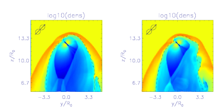
Figure 3: $y$-$z$ section of model A for $\gamma_{1}=5/3$ (left) and $\gamma_{1}=4/3$ (right), while $\gamma_{2}=5/3$. The shock morphology is the same. The system has not yet reached steady state, as can be seen by the ripples in the BS and CD.

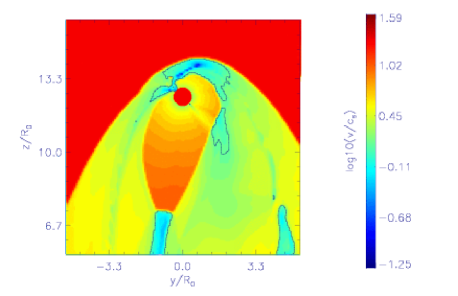
Figure 4: The ratio of total velocity $v=(v_{x}^{2}+v_{y}^{2}+v_{z}^{2})^{1/2}$ to adiabatic sound speed $c_{s}=(\gamma p/\rho)^{1/2}$ in a $y$-$z$ section of model A. The colors denote $v/c_{s}$ in logarithmic scale, as indicated by the color bar. The bulk flow is highly supersonic along, and nearly everywhere within, the boundaries. The solid lines denote the contour levels where $v/c_{s}=1$.

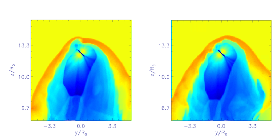
Figure 5: $y$-$z$ sections of model A with a computational domain of $x_{\mathrm{max}}-x_{\mathrm{min}}=y_{\mathrm{max}}-y_{\mathrm{min}}=z_{\mathrm{max}}-z_{\mathrm{min}}=10.6R_{0}$ (left) and the same model with a domain of $x_{\mathrm{max}}-x_{\mathrm{min}}=y_{\mathrm{max}}-y_{\mathrm{min}}=z_{\mathrm{max}}-z_{\mathrm{min}}=21.3R_{0}$ (right, zoomed-in to allow comparison with the left figure) at $t=3.38\tau_{0}$ and $t=3.35\tau_{0}$, respectively. The colors denote the density in logarithmic scale as in figure 2. The shock morphology shows slight differences that can be attributed to the different evolution of the KH instabilities (due to the different resolution of the wind region and the time when the snapshot is taken). We do not observe any back reaction effects in the larger computational domain.

Figure 4 displays the Mach number $v/c_{s}$ [where $c_{s}=(\gamma p/\rho)^{1/2}$ is the adiabatic sound speed] as a function of position in a $y$-$z$ section of model A. The flow is supersonic nearly everywhere along the boundaries and on the pulsar side of the BS. The only exception is a few small regions of subsonic flow in the PS (solid contours in figure 4) and we do not expect the back reaction from these subsonic inclusions to affect the flow structure. In order to verify this claim, we perform one simulation with the parameters of model A and a larger computational domain ($x_{\mathrm{max}}-x_{\mathrm{min}}=y_{\mathrm{max}}-y_{\mathrm{min}}=z_{\mathrm{max}}-z_{\mathrm{min}}=21.3R_{0}$, compared to $x_{\mathrm{max}}-x_{\mathrm{min}}=y_{\mathrm{max}}-y_{\mathrm{min}}=z_{\mathrm{max}}-z_{\mathrm{min}}=10.6R_{0}$ in figure 2) and compare the results in figure 5. We restrict the runtime to $t=3.38\tau_{0}$ (where $\tau_{0}$ is the time for the ISM to cross the visible domain) to keep the computation tractable. Although there are slight changes in the shock structure, which can be attributed to the different resolution of the wind region, we do not see any evidence for back reaction (e.g., matter or sound waves travelling into the visible domain).

3.3 Shock asymmetries

The analytic solution (A) (solid curve in figure 2) approximates the shape of the CD (dashed curve) reasonably well. Here, and in all the following plots, the CD in the simulation is defined by the condition $X_{2}=0.9$ [see equation (5)]. Plainly, the CD in figure 2 is asymmetric. The kink that appears in the analytic solution at the latitude where $\rho_{w}v_{w}^{2}$ is a minimum ($\theta=\pi/2$, perpendicular to $\mathbf{\Omega}$ in the figure) is less distinct in the simulations, because the thermal pressure in the wind and the ISM smoothes out sharp features. Hence, even a highly anisotropic wind does not lead to large, easily observable, kink-like asymmetries in the CD, an important (if slightly disappointing) point to bear in mind when interpreting PWN observational data.

The point of the BS closest to the pulsar is no longer along $\mathbf{v}_{p}$ but depends also on the latitude where the momentum flux is a minimum. However, the BS itself is also smoothed by thermal pressure so it is not a good gauge of the underlying anisotropy. Equally, it is difficult to infer the density of the ambient ISM from the location of the stagnation point, defined as the intersection point of $\mathbf{v}_{p}$ with the BS, since the orientation of $\mathbf{\Omega}$ cannot be inferred uniquely from the shape of the BS.

The asymmetry of the BS in figure 2, which is more extended towards the right side of the figure, is caused by the excess momentum flux along $-\mathbf{v}_{m}$ on this side. Bucciantini (2002) showed that the analytic formula (13) accurately describes the CD for isotropic momentum flux. We confirm here that the analogous formula (A) accurately describes the CD for anisotropic momentum flux. But, as the wind ram pressure decreases downstream from the apex, the thermal pressure becomes increasingly important and the analytic solution breaks down. Nevertheless, the asymmetry is preserved. Likewise, the analytic solution for the BS (dotted curve) deviates more strongly as one moves further downstream from the apex. Again, this result is expected, since the analytic approximation relies on mechanical momentum flux balance and breaks down as the thermal pressure becomes increasingly important.

Momentum flux anisotropy affects the BS weakly, but it affects the structure of the inner flow strongly. A striking feature of figure 2 is the shape of the TS. It is highly asymmetric and elongated, roughly aligned with $\mathbf{\Omega}$. As the rear surface of the TS lies well inside the BS, its position is determined by the balance between the wind ram pressure and the thermal pressure in the PS region, which is found empirically to be roughly the same as in the ISM (Bucciantini, 2002). This, combined with the small momentum flux at $\theta=-\pi/2$ (running diagonally from the upper left to bottom right in figure 2), explains why the side surfaces of the TS are confined tightly, and hence its characteristic convex shape.

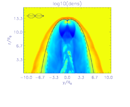
Figure 6: $y$-$z$ section of model B. The colors denote the density in logarithmic scale, as defined in figure 2. The solid curve shows the theoretical solution (A), scaled to match the CD (dashed curve). The solid and dashed curves overlap almost perfectly. The symbol in the top left indicates the projected wind symmetry axis and momentum flux (polar plot), as in the caption of figure 2. Note the butterfly-like TS and the BS almost touching the pulsar.

We now contrast the above results with a system that is axisymmetric around $z$. Figure 6 shows the $y$-$z$ section of model B, which is the same as model A, except that $\mathbf{\Omega}$ is now perpendicular to $\mathbf{v}_{m}$. Not surprisingly, the BS and CD are axisymmetric. The analytic formula (A) describes the CD reasonably well, although the BS deviates slightly near the apex for the pressure-related reasons discussed above. The butterfly-like shape of the TS directly reflects the momentum flux and is a good observational probe in this situation. Note that the CD and BS nearly touch the pulsar at $\theta=-\pi/2$ (where the momentum flux is zero). This illustrates that an estimate of $\rho_{m}$ based on equation (8) and the assumption of an isotropic wind is too low. Note again the KH instabilites at the CD and the blobs of ISM matter in the PS region, which are numerical artifacts.

An example of the difficulties arising from the degeneracy of the problem is PSR J2124$-$3358 (Gaensler et al., 2002). The PWN around this pulsar shows a clear asymmetry near the apex. Gaensler et al. (2002) showed that several combinations of an ISM density gradient (perpendicular and parallel to $\mathbf{v}_{m}$), an ISM bulk flow, and an anisotropic pulsar wind can explain the observed anisotropy, but only in combination, not alone.

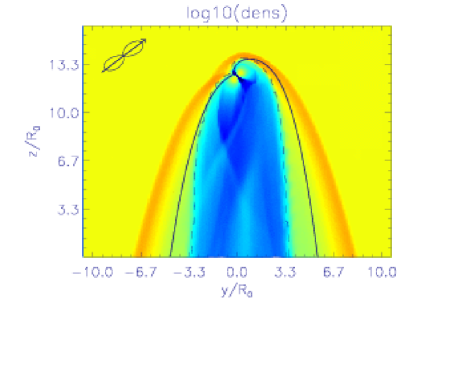
Figure 7: $y$-$z$ section of model C. The colors denote the density in logarithmic scale, as defined in figure 2. The symbol in the top left indicates the projected wind symmetry axis and momentum flux (polar plot), as in the caption of figure 2. The solid curve shows the theoretical solution (A), scaled to match the CD (dashed curve). The momentum flux in the wind is highly collimated, with $g_{w}\propto\cos^{4}\theta$.

Figure 7 demonstrates what the BS looks like when the wind is highly collimated along $\mathbf{\Omega}$, i.e. a jet ($g_{w}\propto\cos^{4}\theta$). Basically, the situation is similar to model A (figure 2): the analytic formula correctly predicts the shape of the CD. However, the kink at the latitude of the momentum flux minimum is less visible than in figures 2 and 6. Moreover, the wind cavity is smaller than in figure 2. The TS approaches the pulsar more closely from behind, where there is less wind momentum flux than in models A and B due to the high collimation. The TS is also confined more tightly by the ISM ram pressure.

3.4 Split-monopole versus wave-like wind

In principle, the results above afford a means of distinguishing between wind models with different momentum flux distributions. In reality, however, the conclusion from section 3.3 and figure 2, that the shapes of the CD and BS depend weakly on $g_{w}(\theta)$, seriously hampers this sort of experiment. For example, the wave-like dipole wind analyzed by Melatos & Melrose (1996) and Melatos (1997) predicts $g_{w}(\theta)=\cos^{2}\theta+1$ (for a point dipole, as calculated in appendix B), while the split-monopole wind analyzed by Bogovalov (1999) predicts $g_{w}(\theta)=\sin^{2}\theta+1/\sigma$, yet these models produce very similar shapes for the CD and BS, as we now show.

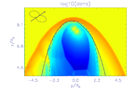
Figure 8: $y$-$z$ section of model A1. The colors denote the density in logarithmic scale, as defined in figure 2. The symbol in the top left indicates the projected wind symmetry axis and the momentum flux (polar plot), as in the caption of figure 2. The solid curve shows the theoretical solution (A), scaled to match the CD (dashed curve). This model describes a wind whose momentum flux is concentrated in the equatorial plane, with $g_{w}(\theta)=\sin^{2}\theta+7/3$

.

Consider an equatorially dominated wind, $c_{2}=-1$, implying $g_{w}(\theta)=7/3+\sin^{2}\theta$. This sort of wind is favored by some PWN observations (Chatterjee & Cordes, 2002). Figure 8 shows the $y$-$z$ section of model A1. We can hardly see any characteristic features in the bow shock. The CD is still described by the analytic solution. The TS looks similar to the TS in model A, mirrored along the $x$-$z$ plane. Indeed, this simulation strongly resembles the situation of a pole-dominated flux with $\lambda=135$° (cf. $\lambda=45\degr$ in model A). We conclude that it will be hard to distinguish these cases observationally.

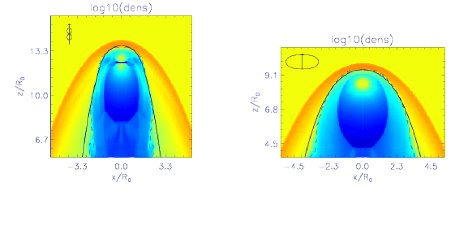
Figure 9: $x$-$z$ section of model A (left) and model A1 (right). The colors denote the density in logarithmic scale, as defined in figure 2. The symbol in the top left indicates the wind symmetry axis, as in the caption of figure 2. The solid curve shows the theoretical solution (A), scaled to match the CD (dashed curve).

Out of interest, a comparison between the $y$-$z$ section and $x$-$z$ section of these models can, in principle, reveal the underlying wind structure. Such a comparison is depicted in figure 9. The pole-dominated wind (left panel) has an anisotropic TS, while the TS in the equatorially-dominated wind (right panel) resembles a completely isotropic outflow. Unfortunately, such a comparison requires orthogonal lines of sight and is not accessible by observation. The computation of synchrotron emission maps for both situations from different angles may provide additional information, if Doppler boosting and column density effects break the degeneracy in figure 8. However, reliable synchrotron maps require RMHD simulations and lie outside the scope of this paper.

4 Cooling

4.1 Numerical implementation

The analytic solution derived by Wilkin (1996, 2000) is exact in the single-layer, thin-shock limit, where both the shocked ISM and the wind cool radiatively (via spectral line emission and synchrotron radiation respectively) faster than the characteristic flow time-scale. In this section, we quantify how rapidly such cooling must occur for the thin-shock approximation to be valid. We also present some simulations of shocks where cooling is not efficient and draw attention to how the structure of these shocks differs from the predictions of Wilkin (2000).

Flash implements optically thin cooling by adding a sink term $-\Lambda(\mathbf{x},t)$ to the right-hand side of equation (3). Radiation is emitted from an optically thin plasma at a rate per unit volume $\Lambda(T)=X_{0}(1-X_{0})\rho^{2}m_{p}^{-2}P(T)$, where $\rho$ is the density, $X_{0}$ is the ionisation fraction, $m_{p}$ is the proton mass, and $P(T)$ is a loss function that depends on the temperature only (Raymond et al., 1976; Cox & Tucker, 1969; Rosner et al., 1978). In our temperature range, $10^{4}$ K $\leq T\leq 10^{5}$ K, hydrogen line cooling dominates and we can write $P(T)\approx 10^{-22}$ erg s^-1 cm³. The postshock temperature $T_{\mathrm{PS}}$ can be extracted directly from the simulation or estimated from the Bernoulli equation and entropy conservation (Bucciantini & Bandiera, 2001). With the latter approach, the result is $k_{\mathrm{B}}T_{\mathrm{PS}}=3m_{p}v_{p}^{2}/32$, where $k_{\mathrm{B}}$ is Boltzmann’s constant.

For a slowly moving pulsar, like PSR J2124$-$3358 which has $v_{p}=61$ km s^-1 and $\rho_{m}=1.6\times 10^{-24}$ g cm^-3 (Gaensler et al., 2002), we find $T_{\mathrm{PS}}=4.2\times 10^{4}$ K and $\Lambda=6.1\times 10^{-21}$ erg s^-1 cm^-3, if we assume a moderate ionisation fraction $X_{0}=0.2$. The internal energy per unit volume in the postshock flow is $\epsilon=(\gamma-1)^{-1}(N_{a}k_{B}/\bar{A})T\rho=1.4\times 10^{-11}$ erg cm^-3 where $\bar{A}=1$ g is the average molecular mass of the hydrogen plasma, from which we deduce a cooling time $\tau=\epsilon_{p}/\Lambda=2.3\times 10^{9}$ s. In this object, the optical bow shock extends 65″or $l=2.3\times 10^{18}$ cm, implying a flow time $t_{f}=l/v_{p}=3.8\times 10^{11}$ s and hence $\tau\ll t_{f}$. This example shows that cooling is important not only in high-luminosity pulsars and in a high density ISM (Bucciantini & Bandiera, 2001), but also if the shock is sufficiently extended, i.e. if the typical flow time, depending on $\mathbf{v}_{p}$, approaches the typical cooling time, which is a function of $\mathbf{v}_{p}$ and $\rho_{m}$. While Bucciantini & Bandiera (2001) argued that the typical cooling length scale is the width of the BS plus the distance between BS and CD, we include the whole visible BS, allowing a longer time for the shocked ISM to cool. This is justified because the material in the post-BS region continues to cool and participate in the dynamics of the system.

We can perform a similar calculation for a fast pulsar, like PSR J1747$-$2958 (the Mouse) which has $v_{p}=600$ km s^-1 and $\rho_{m}=5.0\times 10^{-25}$ g cm^-3 (Gaensler et al., 2002), corresponding to $T_{\mathrm{PS}}=4.1\times 10^{6}$ K and $\Lambda=1.7\times 10^{-24}$ erg s^-1 cm^-3. The cooling efficiency here is lower than in the previous example, since hydrogen line cooling is slower at high temperatures (Raymond et al., 1976) and $\rho_{m}$ is lower. The cooling time $\tau=1.5\times 10^{14}$ s is long compared to the flow time-scale $t_{f}=1.5\times 10^{10}$ s; the length of the BS is $l=0.3$ pc.

To treat H$\alpha$ cooling properly, one must solve the Boltzmann equation for the neutral atom distribution as a function of position, including the ion-neutral reactions, a calculation which lies beyond the scope of this article. Instead, in order to quantify the overall effects of cooling and verify the validity of the analytic thin-shock approximation, we parameterize the cooling function as

$$\Lambda(\mathbf{x},t)=\Lambda_{0}f\rho\epsilon(\mathbf{x},t),$$ (9)

with $\Lambda_{0}=10^{-7}$ s^-1, such that the dimensionless parameter $f$ controls the local cooling time through $\tau=(\Lambda_{0}f)^{-1}$ (which is then spatially uniform by construction, a crude approximation).

4.2 Shock widths

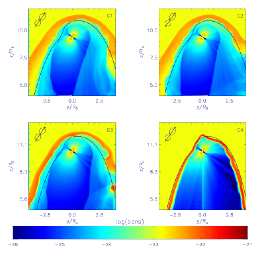
Figure 10: $y$-$z$ section of models C1 ($f=10^{-4}$, upper left), C2 ($f=10^{-3}$, upper right), C3 ($f=10^{-2}$, bottom left), and C4 ($f=1$, bottom right). The colors denote the density in logarithmic scale as indicated by the color bar (g cm^-3), while the solid curve shows the analytic solution (A). The symbol in the top left indicates the projected wind symmetry axis and momentum flux (polar plot), as in the caption of figure 2. For more efficient cooling, e.g. C4, the TS lengthens and the BS becomes thinner, until the TS and BS are no longer separated. The Wilkin (2000) solution (solid curve) matches the bow shock nearly exactly (bottom right), with a deviation of $<8$% from the actual BS position. Here, the bumps at the BS are an artifact of the discrete grid. They are not seen in C1–C3, where small density fluctuations are smoothed by the thermal pressure. However, C1–C3 exhibit strong KH instabilites at the BS.

Figure 10 shows the $y$-$z$ sections of models C1 to C4. These four models are identical ($g_{w}\propto\cos^{2}\theta$, $\lambda=35$°; see table 1), except that $f$ varies from $10^{-4}$ (C1) to $10^{0}$ (C4). For more efficient cooling, the BS becomes thinner (compare upper-left and bottom-right panels in the figure). Similarly, the TS becomes more extended with increasing cooling efficiency, until the wind cavity fills up the BS interior and the TS becomes indistinguishable from the BS for highly efficient cooling (bottom-right panel). Since the pressure in the PS region approximately equals the thermal ISM pressure, and since efficient cooling reduces the PS pressure, the wind ram pressure drives the termination shock outward as $f$ increases, as seen in figure 10. On the other hand, the thickness of the bow shock is controlled by the ratio between the thermal and ram pressures in the ISM. The BS region therefore becomes thinner for more efficient cooling, as we pass from model C1 to C4. For $f=1$, the TS and BS almost touch and the one-layer, thin-shock analytic solution given by equation (A) applies as in the lower-right panel of figure 10.

5 Smooth ISM Density Gradient

Density gradients in the ISM have been invoked to explain the asymmetric features observed in the bow shocks around PSR B0740$-$28, PSR B2224+65 (the Guitar nebula), and PSR J2124$-$3358 (Jones et al., 2002; Chatterjee & Cordes, 2002; Gaensler et al., 2002). The PWN around PSR B0740$-$28 is shaped like a key hole, with a nearly circular head and a divergent tail, starting $\sim 20R_{0}$ downstream from the apex. The Guitar nebula consists of a bright head, an elongated neck, and a limb-brightened body. The PWN around PSR J2124$-$3358 exhibits an asymmetric head and a distinct kink $\sim 10R_{0}$ downstream from the apex.

5.1 Numerical implementation

To explore the effect of a smooth density gradient, we carry out a set of four simulations (D–G in table 1) in which the ISM has an exponential density profile

$$\rho_{m}(y)=\rho_{m,0}\exp(-y/H),$$ (10)

where $H$ is a length scale, and $\rho_{m,0}$ substitutes for $\rho_{m}$ in table 1. We generally choose $H\sim R_{0}\sim 0.01$ pc, consistent with the wavelength of turbulent fluctuations in the warm ISM (Deshpande, 2000). The gradient is perpendicular to the pulsar’s motion. The density profile is initialized and then maintained at later times by setting $\rho_{m}(y)$ at the inflow boundary at $z=z_{\mathrm{max}}$ to $\rho_{m}(y)=\rho_{m,0}\exp(-y/R_{0})$, and choosing $p_{m}$ and $\epsilon_{m}$ consistently. The time-scale over which the associated pressure gradient smoothes out $\rho$, $H/c_{m}\sim 10^{10}$ s, exceeds the flow time-scale, $t_{f}=(z_{\mathrm{max}}-z_{\mathrm{min}})/v_{m}\sim 6\times 10^{9}$ s, so the density gradient remains nearly constant.

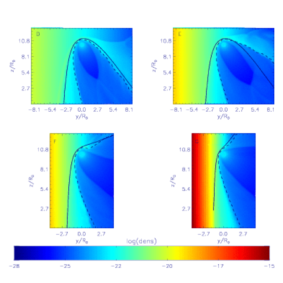
Figure 11: $y$-$z$ sections of model D ($H=1.5R_{0}$, upper left), E ($H=1.0R_{0}$, upper right), F ($H=0.5R_{0}$, lower left), and G ($H=0.25R_{0}$, lower right). The colors denote the density in $\log_{10}$(g cm^-3); note that the color scale differs from that in the other figures. The solid curve shows the theoretical solution (24), scaled to match the CD (dashed curve). The analytic approximation clearly breaks down for models D–G (see text). The BS deviates from the CD where the ISM ram pressure exceeds the thermal pressure. Axes are labelled in units of $R_{0}=1.85\times 10^{16}$ cm.

The analytic solution for the shape of a thin bow shock in an exponential density gradient is given by equation (24).

5.2 Tilted shock

Figure 11 shows the $y$-$z$ sections of models D–G, together with the analytic solution for the BS (solid curve) and the CD (dashed curve). In these models, the exponential density profile changes from shallow ($H=1.5R_{0}$ for model D, upper-left panel) to steep ($H=0.25R_{0}$ for model G, bottom-right panel). One distinctive feature is that the low-density side ($y>0$) of the shock structure, where the CD, TS, and PS are situated, is tilted with respect to $\mathbf{v}_{m}$ by an angle of up to 180° for $H/R_{0}=0.25$. This occurs because the ISM ram pressure, $\rho_{m}v_{m}^{2}$, is dominated by the wind ram pressure for $y>0$, pushing the CD further away from the pulsar. In fact, this part of the CD is approximated well by the analytic formula (24) (Wilkin, 2000). The BS separates from the CD and broadens as the thermal pressure of the ISM in the low-density region increases relative to the ISM ram pressure.

On the high-density side ($y<0$) of the bow shock, the opposite situation prevails. Here, the ram pressure of the ISM exceeds its thermal pressure, so that the BS is well approximated by the thin-shell solution. The CD curves towards the lower density region, pushed by the thermal ISM pressure. The opening angle of the CD increases as $H$ decreases: we find 40°, 60°, 103°, and 124° for models D, E, F, and G respectively, as the ISM ram pressure (for $y>0$) decreases with increasing $y$.

Applying the above results to observations of PWN, we expect the H$\alpha$ surface brightness ($\propto$ column density) to mimic the volume density contours as in Figure 11, especially where the thickness of the BS increases from $y<0$ to $y>0$. Such a variation in the H$\alpha$ flux has not been observed in the PWN around PSR B0740$-$28, PSR B2224+65, and PSR J2124$-$3358 (Jones et al., 2002; Chatterjee & Cordes, 2002; Gaensler et al., 2002). It therefore seems unlikely that a smooth density gradient is responsible for the peculiar morphologies observed in these objects (Chatterjee et al., 2006).

6 Wall in the ISM

The ISM is inhomogenous on length scales from kpc down to AU (Deshpande, 2000). Hence a fast pulsar is likely to encounter singular obstacles or barriers, such as the edges of O-star bubbles (Nazé et al., 2002), which effectively act as “walls”. A wall was invoked to explain the kink observed in the nebula around PSR J2124$-$3358 (Chatterjee et al., 2006). Unlike when a pulsar interacts with its supernova remnant (van der Swaluw et al., 2003), the pulsar does not always strike the wall head on, giving rise to a highly asymmetric interaction.

6.1 Numerical implementation

In order to model the wall, we introduce the (signed) coordinate $\varpi$ along the direction defined by $\cos\alpha\,\hat{\mathbf{y}}-\sin\alpha\,\hat{\mathbf{z}}$, perpendicular to the wall plane. In model W1, the wall is infinitely extended (i.e., a ramp). Its profile can be written as

$$\rho(\varpi)=(\rho_{\mathrm{wall}}-\rho_{m})[1+\exp(\varpi/\Delta_{r})]^{-1}+\rho_{m}.$$ (11)

In models S1 and S2, we truncate the wall on one side. Its profile can be written as

$$\rho(\varpi) = \rho_{m}+(\rho_{\mathrm{wall}}-\rho_{m})[1+\exp(\varpi/\Delta_{r})]^{-1}$$

$$+\theta(-\varpi-8\Delta_{r})(\rho_{\mathrm{wall}}-\rho_{m})\exp[(\varpi+8\Delta_{r})/\Delta_{d}],$$

where $\theta(\varpi)$ is the usual Heaviside function, defined as $\theta(\varpi)=\{0(\varpi<0),1(\varpi\geq 0)\}$. In this notation, $\varpi=0$ denotes the center of the smooth rise in equations (11) and (6.1). The maximum density is $\rho_{\mathrm{wall}}=1.30\times 10^{-23}$ g cm^-3.

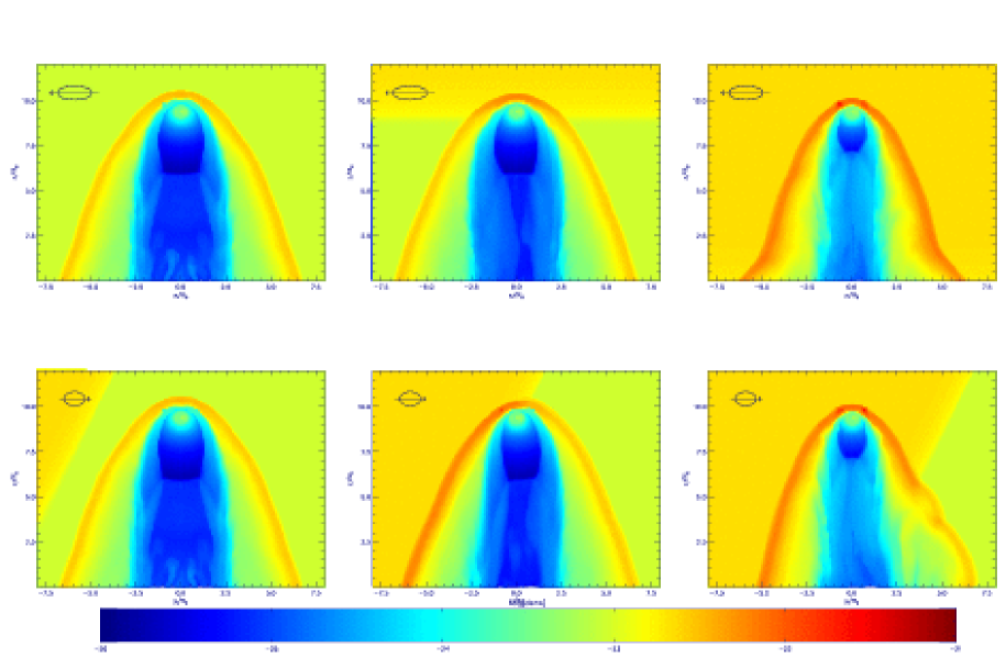
Figure 12: Time series of $x$-$z$ (top row) and $y$-$z$ (bottom row) sections of model W1. The columns are at times $t=1.7t_{f}$ (left), $t=2.5t_{f}$ (middle), and $t=3.4t_{f}$ (right), where $t_{f}=6\times 10^{9}$ s is the time for the ISM to cross the simulation volume. The colors denote the density in $\log_{10}$ (g cm^-3), while the symbol in the top left indicates the projected wind symmetry axis and momentum flux (polar plot), as in the caption of figure 2. The density of the wall is 4 times higher than the ISM density. The momentum flux is anisotropic ($\lambda=90$°) and $\mathbf{\Omega}$ is tilted towards the observer ($\phi=45$°). The bow shock is not disrupted by the wall and shows characteristic kinks and Kelvin-Helmholtz instabilities.

6.2 Kinks in the bow shock

In this section, we examine the effect of a wall on the shock structure and work out how PWN observations probe inhomogenities in the ISM. We consider both a ramp-like [equation (11)] and a truncated [equation (6.1)] wall.

Figure 12 shows a simulation (model W1) where the pulsar hits a ramp-like wall with $\alpha=26$° and density contrast $\eta=\rho_{\mathrm{wall}}/\rho_{m}=2.5$. The wind is asymmetric, with $\lambda=90$°and $\mathbf{\Omega}$ tilted towards the observer ($\phi=45$°), resulting in a slightly asymmetric PS flow. The top and bottom rows of figure 12 depict snapshots of $x$-$z$ and $y$-$z$ sections respectively. The $y$-$z$ sections demonstrate the asymmetry best. On impact, the BS is compressed by the increased ram pressure of the wall. A kink appears at the transition point between the wall and the ambient ISM. Both the gradient in H$\alpha$ brightness and the kink should be observable in principle. As the pulsar proceeds into the high-density region (see middle panels of Figure 12), the CD approaches the pulsar due to the increased ISM ram pressure. Likewise, the ISM thermal pressure increases with increasing $\rho_{m}$ and, by the argument given in section 3.3, the rear surface of the TS comes closer to the pulsar. Just as for a smooth ISM density gradient (cf. Figure 11), the shocks are tilted towards the low density side. When the pulsar proceeds into the densest part of the ISM, the BS, CD, and TS approach even closer to the pulsar until they finally reach the state in the rightmost panels.

In this stationary state, KH instabilites triggered by perturbations during the collision with the wall occur at the right hand surfaces of the CD. In the absence of gravity, the KH instability occurs for all wave numbers and hence on all length-scales down to the grid resolution ($\sim 0.1R_{0}$ in this simulation). However, the collision with the wall introduces a velocity perturbation that is large ($\sim v_{m}$) compared to the numerical noise. This explains why we see the instability in the right panels but not the left panels, where the wall has not yet reached the BS. Indeed, the length scale of the density rise due to the wall agrees with the wavelength of the observed KH instability ($\sim R_{0}$).

In the lower middle panel, the CD downstream from the apex is slightly lopsided towards the higher density (left) side. This occurs because the PS flow from the side surfaces of the TS travels faster than the ISM. The region inside the CD therefore loses pressure support by the shocked wind material, and the shocked ISM material pushes into the space. The same effect can be seen in the lower right panel on the lower density (right) side, where the KH instabilities favor the right-hand side. The top row ($x$-$z$ sections) basically resembles a head-on collision, similar to the interaction of a PWN with the pulsar’s supernova remnant (van der Swaluw et al., 2003). Note also the broadening of the lower part of the BS (top right panel), which demonstrates the delay ($\sim 5R_{0}/v_{m}$) before the shock adjusts to the higher external density $\rho_{m}$.

The H$\alpha$ emission emanates chiefly from the region between the BS and the CD (Bucciantini & Bandiera, 2001), which is only moderately affected by the passing wall. Furthermore, ISM inhomogenities often consist of highly ionised matter (Chatterjee et al., 2006), so that the H$\alpha$ luminosity observed as the wall passes is dominated by the afterglow of the neutral part of the non-wall ISM. Negligible brightness variations are observable in either case. Nevertheless, as we discuss in section 7, a comprehensive treatment of the emission requires the solution of the Boltzmann equation for the neutral and ionized species, a task beyond the scope of this article.

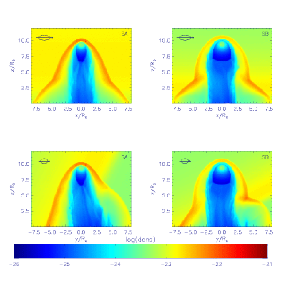
Figure 13: $x$-$z$ (top row) and $y$-$z$ (bottom row) sections of model SA (left column) and model SB (right column). The colors denote the density in $\log_{10}$ (g cm^-3), while the symbol in the top left indicates the projected wind symmetry axis and momentum flux (polar plot), as in the caption of figure 2. In these simulations, the pulsar travels into a wall with a finite width. The momentum flux is anisotropic ($\lambda=90$°) and $\mathbf{\Omega}$ is tilted away from the observer ($\phi=-45$°).

In models SA ($\alpha=26.6$°) and SB ($\alpha=63.4$°), displayed in figure 13, the density ramp is replaced by a wall of finite width, which is truncated as in equation (6.1). The top and bottom row again shows $x$-$z$ and $y$-$z$ sections respectively. As above, the $x$-$z$ sections resemble a head-on collision. The base of the BS broadens in the low-density region and narrows at the density maximum. Above the wall, the BS readjusts to the lower ISM density. Due to the smooth gradient ($\Delta_{d}\gg\Delta_{r}$), the BS looks “egg-shaped”, an effect that can been seen more clearly in the upper-right panel, where the inclination of the wall is lower ($\alpha=64$°). The kink is also more distinct, as seen in the $y$-$z$ sections (lower panels), because the BS expands in the low density region above the wall. The CD and TS approach the pulsar for the same reasons discussed above, but the smooth gradient is responsible for the bulbous shape. Again, as in figure 12, we can see in the lower-right corners of the lower panels how the shocked wind material inside the CD loses pressure support and the shocked ISM material diffuses in.

7 Discussion

In this paper, we perform three-dimensional simulations of pulsar bow shocks in the ISM under a variety of asymmetry-inducing conditions: an anisotropic pulsar wind, an ISM density gradient, and an ISM wall. We validate the analytic solution of Wilkin (1996, 2000) for an anisotropic wind and show that it remains a reasonable approximation for the thick-shock case, with a deviation of $\sim 10$% within $\sim 5R_{0}$ of the apex. We show that the basic multilayer shock structure (TS, CD and BS) obtained by Bucciantini (2002) and Bucciantini et al. (2005) for an isotropic wind is preserved in an anisotropic wind as well. We find that the thermal pressure smoothes the BS. The underlying anisotropy of the momentum flux thus remains concealed, making it difficult to gauge the ISM density from the stagnation point, since generally neither the distribution of the momentum flux nor the orientation of the pulsar spin axis is known.

Contrary to previous estimates (Bucciantini & Bandiera, 2001), we show that cooling can be important for slow pulsars in a low-density ISM, such as PSR J2124$-$3358. This is because the shocked ISM continues to take part in the dynamics of the system and thus influences the overall shape. There are observational consequences: cooling tends to increase the overall size of the TS while the BS becomes thinner. Naively, a thinner BS is expected to be brighter due to limb brightening. However, in order to quantify the effects of cooling on the optical emission, it is necessary to solve the collisionless Boltzmann equation for the neutral hydrogen atoms, a task beyond the scope of this paper.

Our simulations are non-relativistic and do not include the effects of a magnetic field. Bucciantini et al. (2005) showed that a proper relativistic treatment increases the KH instabilities arising at the CD by enhancing the velocity shear at the interface. In principle, therefore, shocked ISM material can contaminate the wind material, altering the inner flow structure and perhaps modulating the synchrotron flux in time, although no simulation has demonstrated the latter effect to date. A magnetic field affects the flow more drastically, in two ways. First, the standoff distance increases because the magnetic field adds to the pressure at the leading surface. This is a runaway process in the simulations of Bucciantini et al. (2005), who neglected resistivity. Second, the TS becomes convex because the magnetic pressure is not uniform. The azimuthal magnetic field builds up near the pulsar, increasing the magnetic pressure. This effect is strongest at $z_{p}$ and decreases as $z$ decreases.

An interesting question is whether the magnetic field in PWN can produce the torus-ring structure found by Komissarov & Lyubarsky (2003, 2004) and Del Zanna et al. (2004), where a jet is formed by circulating back flow of the shocked wind material colliminated subsequently by the magnetic field. This circulation takes place outside the TS and is suppressed by strong confinement in PWN. However, a detailed understanding of the magnetic field structure when the momentum flux is asymmetric must await future simulations.

PWN are commonly detected as radio or X-ray synchrotron sources. Charged wind leptons are accelerated at the termination shock and subsequently gyrate in the local magnetic field, emitting synchrotron radiation. Typically, the emission is observed from three different zones: the TS itself, the PS region, and the head of the BS. For an identification of these zones in the Mouse, see Gaensler et al. (2004). A further theoretical study of the synchrotron emission will be undertaken in a forthcoming paper (Chatterjee et al., 2006). Here, we simply make a few qualitative points.

1. Generally, we observe a variety of TS shapes from inclined tori (Crab Nebula, where the emission is equatorially concentrated) to cylinders (as seen in the Mouse, for a nearly isotropic wind). The emission from the TS depends strongly on the anisotropy of the wind. The more peculiar the shape, the more information it can provide about the inclination of the spin axis with respect to the direction of motion as well as the angular distribution of wind momentum flux. The asymmetry in the TS (figures 2 and 7) directly corresponds to the axis of maximum emission.

2. For isotropic wind emission, one expects the PS flow to be observed as an uncollimated X-ray tail (Bucciantini, 2002). However, if the wind is anisotropic (cf. Figures 2–7), our simulations predict overluminous and underluminous regions (corresponding to high and low densities) in the PS flow, even two separated tails in extreme cases (as in figure 6).

3. The observed appearance of the BS is strongly influenced by the emission from particles accelerated at the head of the BS and subsequently swept back along the CD. Since only the flow component normal to the shock slows down, the flow in the swept-back region is generally trans-relativistic ($\sim c$). If this part of the PS flow [region B1 in Chatterjee et al. (2006)] is laminar along the CD, Doppler beaming may render the emitted radiation invisible (Bucciantini et al., 2005). An anisotropic wind, however, may have a sufficiently large velocity component towards the line of sight to allow detection (Chatterjee et al., 2006). In the case of a jet-like wind, the BS can exhibit a one-sided X-ray tail whose receding half is suppressed by Doppler beaming, as in the PWN around PSR J2124$-$3358 (Chatterjee et al., 2006, whose model B corresponds to our model SA).

Some PWN are also detected in neutral hydrogen emission lines (Gaensler & Slane, 2006). Neutral hydrogen atoms are excited collisionally or by charge exchange and then de-excite radiatively in the region between the BS and CD. Hence, the H$\alpha$ luminosity depends crucially on $\mathbf{v}_{p}$ and $X_{0}$. A proper kinetic (Boltzmann) treatment incorporating ion-neutral reactions is discussed by Bucciantini & Bandiera (2001). It is clear that purely hydrodynamical simulations like ours cannot predict the observed surface brightness reliably. However, in a paper in preparation (Chatterjee et al., 2006), we show that the overall shape of the bow shock is predicted reliably.

If high-resolution observations of the shock apex can resolve the characteristic kink in the BS at the latitude where the momentum flux is a minimum, they will shed light on the angular distribution of the pulsar wind momentum flux and hence the electrodynamics of the pulsar magnetosphere (Bogovalov, 1999; Komissarov & Lyubarsky, 2003, 2004; Melatos & Melrose, 1996; Melatos, 1997, 2002). However, it is generally difficult to distinguish between equatorially dominated (e.g., split-monopole) and pole-dominated (e.g., wave-like dipole) wind models, beacuse the shock structure is degenerate with respect to several parameters and does not depend sensitively on the momentum flux distribution (see sections 3.3 and 3.4). Only for favored inclinations, e.g. when $\mathbf{\Omega}$ points directly towards us and the TS ring is resolved (as in the Crab nebula), can the synchrotron emission from the TS be used to make more definite statements. Again, RMHD simulations for anisotropic winds and synchrotron emission maps are needed to break the degeneracies.

Pulsar bow shocks probe the local small-scale structure of the ISM. An ISM density gradient modifies the shape of the bow shock substantially away from the Wilkin (2000) solution. Since H$\alpha$ emission is generated behind the BS, density fluctuations with a length-scale $\ga R_{0}$ should be clearly visible. If the gradient is nearly perpendicular to $\mathbf{v}_{m}$, we expect the surface brightness of the nebula to be asymmetric as well, even one-sided in extreme cases. In addition, the TS is tilted towards the low density side, producing asymmetric synchrotron emission. Steep density gradients with length-scale $\la R_{0}$ (i.e. walls) produce characteristic kink-like features. For example, a wall consisting of mainly ionized matter can account for the observed shape of the PWN associated with PSR J2124$-$3358 (Chatterjee et al., 2006). If the pulsar encounters a truncated wall with a finite width, the bow shock develops a peculiar shape: an egg-like head and a divergent tail (as in figure 13). This shape is strikingly similar to the H$\alpha$ emission observed from PSR B0740$-$28 (Jones et al., 2002). Multi-epoch observations of the Guitar nebula (Chatterjee & Cordes, 2004) reveal time-dependent behaviour of this PWN that corresponds to the overall situation shown in figure 12 (although not to the time between the snapshots in figure 12, of course, which are separated $\sim 10^{2}$ yr). When the pulsar runs into the higher density region, the wind is confined more strongly and the BS is pushed closer to the pulsar, explaining the narrow head and diverging tail. Furthermore, we note that the Guitar nebula is significantly brighter near the strongly confined head. This can be explained in terms of the increased density of the shocked ISM, if we assume that the high density region carries a neutral fraction comparable to the low density region. On the other hand, our simulations do not exhibit the rear shock seen in the Guitar nebula, which could be due to a higher $\eta$ than considered in models SA and SB.

Summarizing our results, we conclude that the anisotropy of the wind momentum flux alone cannot explain odd bow shock morphologies. Instead, it is necessary to take into account external effects, like ISM density gradients or walls. Conversely, because the shape of the bow shock is degenerate with respect to several parameters, it is difficult to infer the angular distribution of the wind momentum flux from the H$\alpha$ radiation observed. Highly resolved radio and X-ray observations, combined with synchrotron emission maps from RMHD simulations, may break these degeneracies in the future. Finally, we caution the reader that the results presented here explore a very limited portion of the (large) parameter space of the problem.

Appendix A Analytic bow shock formulas in the thin-shell limit

Wilkin (1996) showed that the shape of the CD when the pulsar wind momentum flux is isotropic can be written as:

$$R(\theta)=R_{0}\csc\theta[3(1-\theta\cot\theta)]^{1/2}$$ (13)

in the limit of a thin shock. Here, $R(\theta)$ gives the distance from the pulsar position to the bowshock, $\theta$ denotes the colatitude measured relative to the orientation of the symmetry axis (see section 3), and $R_{0}$ is the standoff distance defined in equation (8).

The formalism was extended to an anisotropic pulsar wind with $p=2$, by Wilkin (2000), who found

$$R(\theta) = R_{0}\csc\theta^{\prime}\{3(1-\theta^{\prime}\cot\theta^{\prime})[c_{0}+\frac{c_{2}}{4}(3v^{2}+w^{2})]$$

$$+\frac{3c_{2}}{4}[(v^{2}-w^{2})\sin^{2}\theta^{\prime}+vw(2\theta^{\prime}-\sin 2\theta^{\prime})]\}^{1/2},$$

with $v=\sin\phi^{\prime}\sin\lambda$, $w=\cos\lambda$, and $c_{0}=1-c_{2}/3$, if the momentum flux is of the form $\rho_{w}(\theta)=\rho_{0,w}(c_{0}+c_{2}\cos^{p}\theta)$ as in equation (7). $\theta^{\prime}$ and $\phi^{\prime}$ are the usual spherical coordinates with respect to the $z$ axis, such that

$$\cos\theta=v\sin\theta^{\prime}+w\cos\theta^{\prime}.$$ (15)

Note that this notation differs from Wilkin (2000): his $\theta_{\ast}$ corresponds to our $\theta$, while his $\theta$ and $\phi$ correspond to our $\theta^{\prime}$ and $\phi^{\prime}$ respectively.

We derive a formula for $R(\theta)$ in the case $p=4$ by applying the formalism of Wilkin (2000). The case $p=4$ is relevant to a collimated jet (Chatterjee et al., 2006) or an extended vacuum dipole (see appendix B). Inside the wind cavity, the momentum flux can be written as (Wilkin, 2000)

$$\rho_{w}(r,\theta)v_{w}^{2}=\frac{\dot{E}}{2\pi r^{2}v_{w}}g_{w}(\theta),$$ (16)

with

$$g_{w}(\theta)=c_{0}+c_{2}\cos^{4}\theta.$$ (17)

Here, the overall energy loss $\dot{E}$ is related to the simulation parameters $\rho_{0,w}$ and $r_{w}$ through $\dot{E}=2\pi r_{w}^{2}\rho_{0,w}v_{w}^{3}$. The normalisation

$$\int_{0}^{2\pi}\mathrm{d}\phi\int_{0}^{\pi}\mathrm{d}\theta\,\sin\theta\,g_{w}(\theta)=4\pi$$ (18)

requires $c_{0}=1-c_{2}/5$ for $p=4$. The incident momentum flux from the wind on the shell can then be written as

$$\mathbf{\Phi}_{w}(\theta^{\prime},\phi^{\prime})=\frac{\dot{E}}{2\pi v_{w}}\mathbf{G}_{w}(\theta^{\prime},\phi^{\prime}).$$ (19)

Here, $\mathbf{G}_{w}=G_{w,\varpi}\hat{\mn@boldsymbol{\varpi}}+G_{w,z}\hat{\mathbf{z}}$, where the cylindrical coordinates $\varpi$ and $z$ are defined with respect to the symmetry axis, is a dimensionless function given by

$$\mathbf{G}_{w}=\int_{0}^{\theta^{\prime}}\mathrm{d}\theta^{\prime\prime}\,g_{w}(\hat{\mn@boldsymbol{\varpi}}\sin\theta^{\prime\prime}+\hat{\mathbf{z}}\cos\theta^{\prime\prime})\sin\theta^{\prime\prime}.$$ (20)

From (15) and (17), we can compute $g_{w}$ and hence $\mathbf{G}_{w}$ as a function of $\theta^{\prime}$ and $\phi^{\prime}$:

$$g_{w}=c_{0}+c_{2}(\sin\theta^{\prime}v+\cos\theta^{\prime}w)^{4}.$$ (21)

It can now be shown (Wilkin, 2000) that the bow shock shape is described by

$$R(\theta^{\prime},\phi^{\prime})=R_{0}\csc\theta^{\prime}[-6(G_{w,\varpi}\cot\theta^{\prime}-G_{w,z})]^{1/2}.$$ (22)

Substituting (20) and (21) into (22) finally yields

$$R = \frac{R_{0}}{8}\csc\theta^{\prime}\{-\csc\theta^{\prime}\{c_{0}[192\theta^{\prime}\cos\theta^{\prime}-192\sin\theta^{\prime}]$$

$$+c_{2}[vw^{3}(16\cos\theta^{\prime}-12\cos 3\theta^{\prime}-4\cos 5\theta^{\prime}-96\theta^{\prime}\sin\theta^{\prime})$$

$$+v^{3}w(32\cos\theta^{\prime}-36\cos 3\theta^{\prime}+4\cos 5\theta^{\prime}-96\theta^{\prime}\sin\theta^{\prime})$$

$$+v^{2}w^{2}(144\theta^{\prime}\cos\theta^{\prime}-168\sin\theta^{\prime}+18\sin 3\theta^{\prime}-6\sin 5\theta^{\prime})$$

$$+v^{4}(120\theta^{\prime}\cos\theta^{\prime}-80\sin\theta^{\prime}-15\sin 3\theta^{\prime}+\sin 5\theta^{\prime})$$

$$+w^{4}(24\theta^{\prime}\cos\theta^{\prime}-56\sin\theta^{\prime}+9\sin 3\theta^{\prime}+\sin 5\theta^{\prime})]\}\}^{1/2}.$$

Figure 14: Comparison of the bow shock shape for $p=2$ (left) and $p=4$ (right), given $\lambda=\pi/4$, $c_{0}=0$ and $c_{2}=3$. We note the strong similarity between these solutions, the only difference being the slimmer shape for $p=4$.

Figure 14 shows the two solutions (A) and (A) for $\lambda=\pi/4$, $c_{0}=0$, and $c_{2}=3$. Although the shapes are nearly identical, the $p=4$ surface is slimmer. The difference is seen more clearly in figure 15, which shows the $y$-$z$ section of the bow shock. The $p=4$ case (dashed curve) touches the $p=2$ shock (solid curve) at the latitude of maximum momentum flux, $\theta=\pi/4$ (upper-right corner). Both surfaces show a characteristic kink at the latitude where the momentum flux is a minimum.

Figure 15: $y$-$z$ section of the bow shock for $p=2$ (solid curve) and $p=4$ (dashed curve). The strong similarity hampers efforts to distinguish between the two cases observationally.

By a similar calculation, we can derive the shape of the BS for an exponential density gradient perpendicular to $\mathbf{v}_{m}$ (Wilkin, 2000). The result is

$$R(\theta,\phi)=H\sec\phi\sin^{-1}\theta y_{s}(\theta,\phi),$$ (24)

where $y_{s}$ is the solution of

$$\frac{1}{y}\left[y-2+\exp(-y)(y+2)\right]=\frac{1}{6}y_{\mathrm{ax}}^{2}$$ (25)

and $y_{\mathrm{ax}}$ is the normalised standoff distance,

$$y_{\mathrm{ax}}=\frac{R_{0}}{H}\cos\phi[3(1-\theta\cot\theta)]^{1/2}.$$ (26)

Appendix B Angular distribution of the momentum flux for an extended vacuum dipole

Although the electrodynamics of the pulsar magnetosphere and wind remain unsolved, it is commonly assumed that the angular distribution of the energy flux at the light cylinder is preserved in the transition to a kinetic-energy-dominated outflow at the TS (Del Zanna et al., 2004). In this appendix, we calculate the far-field Poynting flux for point-like and extended dipoles rotating in vacuo.

The relevant electromagnetic far field components are given by the real parts of the following expressions (Melatos, 1997):

$$B_{\theta}=\frac{\mathrm{i}B_{0}}{2x}\left[a(x_{0})-b(x_{0})\right]\sin\alpha\cos\theta\mathrm{e}^{\mathrm{i}(x+\eta)}+O(x^{-2}),$$ (27)

$$B_{\phi}=-\frac{B_{0}}{2x}\left[a(x_{0})\cos 2\theta-b(x_{0})\right]\sin\alpha\mathrm{e}^{\mathrm{i(x+\eta)}}+O(x^{-2}),$$ (28)

$$(E_{\theta},E_{\phi})=c(B_{\phi},-B_{\theta}).$$ (29)

In (27)–(29), $x=\omega r/c$ denotes a normalized radial coordinate, $\omega$ is the pulsar’s angular velocity, $x_{0}=\omega r_{0}/c$ is the normalized effective radius of the corotating magnetosphere, $\eta=\phi-\omega t$ is the phase of the electromagnetic wave, and $B_{0}$ is the magnitude of the stellar magnetic field at the poles. Constants $a$ and $b$ are given by

$$a=\frac{x_{0}^{2}}{x_{0}h_{2}^{\prime}(x_{0})+h_{2}(x_{0})}$$ (30)

and

$$b=\frac{x_{0}}{h_{1}(x_{0})},$$ (31)

where $h_{1}(x)$ and $h_{2}(x)$ are the first and second-order spherical Hankel functions of the first kind. The $r$ component of the Poynting flux can then be computed from

$$\mathbf{S}_{r} = \frac{1}{2\mu_{0}}(\mathbf{E}\times\mathbf{B^{*}})_{r}$$ (32)

$$= S_{0}(|a-b|^{2}\cos^{2}\theta+|a\cos 2\theta-b|^{2})\sin^{2}\alpha$$

with $S_{0}=(c/2\mu_{0})(B_{0}/2x)^{2}$.

We can simplify (32) using the explicit form of the Hankel functions,

$$h_{1}(x)=\mathrm{e}^{\mathrm{i}x}\left(-\frac{1}{x}-\frac{\mathrm{i}}{x^{2}}\right)$$ (33)

and

$$h_{2}(x)=\mathrm{e}^{\mathrm{i}x}\left(\frac{\mathrm{i}}{x}-\frac{3}{x^{2}}-\frac{3\mathrm{i}}{x^{3}}\right).$$ (34)

In the case of a point dipole, we have $x_{0}\ll 1$. Retaining the leading order terms, we obtain

$$a=-\frac{\mathrm{i}}{6}x_{0}^{5}\mathrm{e}^{-\mathrm{i}x_{0}},$$ (35)

$$b=-\mathrm{i}x_{0}^{3}\mathrm{e}^{-\mathrm{i}x_{0}},$$ (36)

and hence

$$\mathbf{S}_{r}=S_{0}x_{0}^{6}(\cos^{2}\theta+1)\sin^{2}\alpha,$$ (37)

which reduces to the case $p=2$, $c_{0}=c_{2}=1$ in Wilkin (2000).

We also calculate the Poynting flux for an extended dipole, as proposed by Melatos (1997). For the special case $x_{0}=1$, an explicit calculation yields

$$\mathbf{S}_{r}=\frac{S_{0}}{17}(2\cos^{4}\theta+6\cos^{2}\theta+5)\sin^{2}\alpha.$$ (38)

References

- Arons (2004) Arons J., 2004, Advances in Space Research, 33, 466
- Bell et al. (1995) Bell J. F., Bailes M., Manchester R. N., Weisberg J. M., Lyne A. G., 1995, ApJ, 440, L81
- Bogovalov (1999) Bogovalov S. V., 1999, A&A, 349, 1017
- Bogovalov et al. (2005) Bogovalov S. V., Chechetkin V. M., Koldoba A. V., Ustyugova G. V., 2005, MNRAS, 358, 705
- Bucciantini (2002) Bucciantini N., 2002, A&A, 387, 1066
- Bucciantini (2006) Bucciantini N., 2006, astro-ph/0608258
- Bucciantini et al. (2005) Bucciantini N., Amato E., Del Zanna L., 2005, A&A, 434, 189
- Bucciantini & Bandiera (2001) Bucciantini N., Bandiera R., 2001, A&A, 375, 1032
- Chatterjee & Cordes (2002) Chatterjee S., Cordes J. M., 2002, ApJ, 575, 407
- Chatterjee & Cordes (2004) Chatterjee S., Cordes J. M., 2004, ApJ, 600, L51
- Chatterjee et al. (2006) Chatterjee S., et al., 2006, in preparation
- Chatterjee et al. (2005) Chatterjee S., Vlemmings W. H. T., Brisken W. F., Lazio T. J. W., Cordes J. M., Goss W. M., Thorsett S. E., Fomalont E. B., Lyne A. G., Kramer M., 2005, ApJ, 630, L61
- Chevalier et al. (1980) Chevalier R. A., Kirshner R. P., Raymond J. C., 1980, ApJ, 235, 186
- Chevalier & Raymond (1978) Chevalier R. A., Raymond J. C., 1978, ApJ, 225, L27
- Cordes et al. (1993) Cordes J. M., Romani R. W., Lundgren S. C., 1993, Nature, 362, 133
- Coroniti (1990) Coroniti F. V., 1990, ApJ, 349, 538
- Cox & Tucker (1969) Cox D. P., Tucker W. H., 1969, ApJ, 157, 1157
- Del Zanna et al. (2004) Del Zanna L., Amato E., Bucciantini N., 2004, A&A, 421, 1063
- Deshpande (2000) Deshpande A. A., 2000, MNRAS, 317, 199
- Fryxell et al. (2000) Fryxell B., et al., 2000, ApJS, 131, 273
- Gaensler et al. (2002) Gaensler B. M., Arons J., Kaspi V. M., Pivovaroff M. J., Kawai N., Tamura K., 2002, ApJ, 569, 878
- Gaensler et al. (2002) Gaensler B. M., Jones D. H., Stappers B. W., 2002, ApJ, 580, L137
- Gaensler & Slane (2006) Gaensler B. M., Slane P. O., 2006, Annu. Rev. of Astron. & Astrophys., 44, 17
- Gaensler et al. (2004) Gaensler B. M., van der Swaluw E., Camilo F., Kaspi V. M., Baganoff F. K., Yusef-Zadeh F., Manchester R. N., 2004, ApJ, 616, 383
- Ghavamian et al. (2001) Ghavamian P., Raymond J., Smith R. C., Hartigan P., 2001, ApJ, 547, 995
- Goldreich & Julian (1969) Goldreich P., Julian W. H., 1969, ApJ, 157, 869
- Helfand et al. (2001) Helfand D. J., Gotthelf E. V., Halpern J. P., 2001, ApJ, 556, 380
- Hobbs et al. (2005) Hobbs G., Lorimer D. R., Lyne A. G., Kramer M., 2005, MNRAS, 360, 974
- Jones et al. (2002) Jones D. H., Stappers B. W., Gaensler B. M., 2002, A&A, 389, L1
- Kaspi et al. (2004) Kaspi V. M., Roberts M. S. E., Harding A. K., 2004, to appear in: Compact Stellar X-ray Sources, ed: Lewin, W.H.G. & van der Klis, M. astro-ph/0402136
- Kennel & Coroniti (1984a) Kennel C. F., Coroniti F. V., 1984a, ApJ, 283, 694
- Kennel & Coroniti (1984b) Kennel C. F., Coroniti F. V., 1984b, ApJ, 283, 710
- Komissarov & Lyubarsky (2003) Komissarov S. S., Lyubarsky Y. E., 2003, MNRAS, 344, L93
- Komissarov & Lyubarsky (2004) Komissarov S. S., Lyubarsky Y. E., 2004, MNRAS, 349, 779
- Kulkarni & Hester (1988) Kulkarni S. R., Hester J. J., 1988, Nature, 335, 801
- Loehner (1987) Loehner R., 1987, Comp. Meth. App. Mech. Eng., 61, 323
- Luo et al. (1990) Luo D., McCray R., Mac Low M.-M., 1990, ApJ, 362, 267
- Melatos (1997) Melatos A., 1997, MNRAS, 288, 1049
- Melatos (2002) Melatos A., 2002, in Slane P. O., Gaensler B. M., eds, ASP Conf. Ser. 271: Neutron Stars in Supernova Remnants Theory of Plerions. pp 115–+
- Melatos et al. (1995) Melatos A., Johnston S., Melrose D. B., 1995, MNRAS, 275, 381
- Melatos & Melrose (1996) Melatos A., Melrose D. B., 1996, MNRAS, 279, 1168
- Melatos et al. (2005) Melatos A., Scheltus D., Whiting M. T., Eikenberry S. S., Romani R. W., Rigaut F., Spitkovsky A., Arons J., Payne D. J. B., 2005, ApJ, 633, 931
- Nazé et al. (2002) Nazé Y., Chu Y.-H., Guerrero M. A., Oey M. S., Gruendl R. A., Smith R. C., 2002, AJ, 124, 3325
- Olson et al. (1999) Olson K. M., MacNeice P., Fryxell B., Ricker P., Timmes F. X., Zingale M., 1999, Bulletin of the American Astronomical Society, 31, 1430
- Raymond et al. (1976) Raymond J. C., Cox D. P., Smith B. W., 1976, ApJ, 204, 290
- Roberts et al. (2003) Roberts M. S. E., Tam C. R., Kaspi V. M., Lyutikov M., Vasisht G., Pivovaroff M., Gotthelf E. V., Kawai N., 2003, ApJ, 588, 992
- Rosner et al. (1978) Rosner R., Tucker W. H., Vaiana G. S., 1978, ApJ, 220, 643
- Spitkovsky & Arons (1999) Spitkovsky A., Arons J., 1999, Bulletin of the American Astronomical Society, 31, 1417
- Spitkovsky & Arons (2004) Spitkovsky A., Arons J., 2004, ApJ, 603, 669
- Stappers et al. (2003) Stappers B. W., Gaensler B. M., Kaspi V. M., van der Klis M., Lewin W. H. G., 2003, Science, 299, 1372
- van der Swaluw et al. (2003) van der Swaluw E., Achterberg A., Gallant Y. A., Downes T. P., Keppens R., 2003, A&A, 397, 913
- van Kerkwijk & Kulkarni (2001) van Kerkwijk M. H., Kulkarni S. R., 2001, A&A, 380, 221
- Wilkin (1996) Wilkin F. P., 1996, ApJ, 459, L31+
- Wilkin (2000) Wilkin F. P., 2000, ApJ, 532, 400