December 24, 2006

Astrophysics of Wormholes
 
N.S. Kardashev¹, I.D. Novikov^1,2, and A.A. Shatskiy¹

¹ Astro Space Center, Lebedev Physical Institute, Russian Academy of Sciences,
Profsoyuznaya ul., 84/32, Moscow, 117997, RUSSIA.
² Niels Bohr Institute, Blegdamsvej 17, DK-2100, Copenhagen Denmark.

ABSTRACT
We consider the hypothesis that some active galactic nuclei and other compact astrophysical objects may be current or former entrances to wormholes. A broad mass spectrum for astrophysical wormholes is possible. We consider various new models of the static wormholes including wormholes maintained mainly by an electromagnetic field. We also discuss observational effects of a single entrance to wormhole and a model for a binary astrophysical system formed by the entrances of wormholes with magnetic fields and consider its possible manifestation.

1 INTRODUCTION

The purpose of this paper is to consider a possibility that some astrophysical objects may be current or former entrances to wormholes (WHs). These wormholes may be relic of the inflation epoch of the evolution of the Universe [1] - [9] and fig. 1.

It follows from WH models that their existence requires matter with a peculiar equation of state [10]-[14]. This equation must be anisotropic, and ${w_{\parallel}=p_{\parallel}/\varepsilon}$ must be smaller than ${-1}$, as in the case of phantom matter (${p_{\parallel}}$ is the total pressure along the tunnel of the WH, and ${\varepsilon}$ is the total energy density for all components of the matter in the tunnel of the WH). The existence of such matter remains hypothetical [15]. For definiteness, we will use the term ”phantom energy”  for an isotropic equation of state ${p/\varepsilon<-1}$, and the term ”phantom matter”  for an anisotropic equation of state. The units are selected so that ${c=1}$ and ${G=1}$ (with exceptions for final relations).

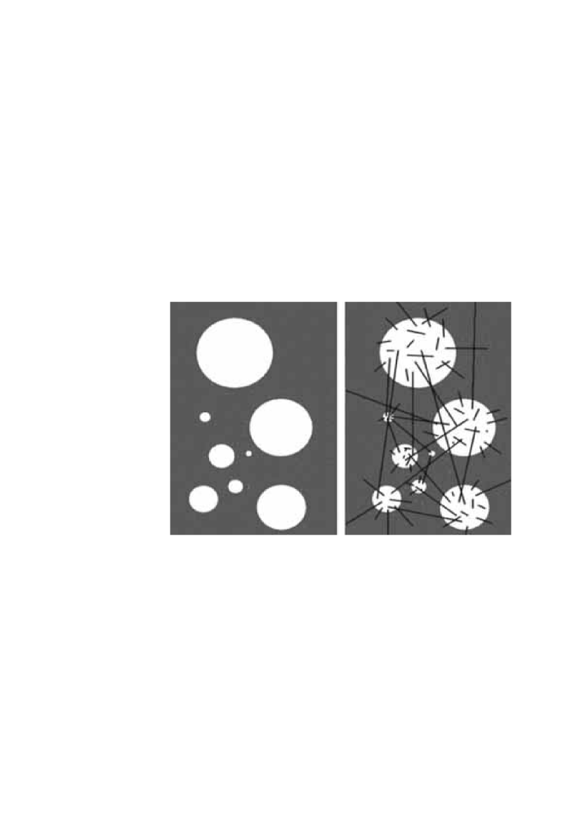
Figure 1: Model of chaotic inflation in a multi-element Universe without (left) and with (right) wormholes.

In this paper we consider a model in which the main component of a wormhole having all the necessary properties is a strong magnetic field that penetrates the WH, while phantom matter and phantom energy are required only in small amounts. We also consider a model based on phantom energy, where the equation of state is close to that for a vacuum ${(p/\varepsilon=-1)}$, with some added energy density of the magnetic field.

We do not consider here the dynamics of wormholes. Thus all conditions for the relations between the components of the stress-energy tensor correspond to the static state but not dynamics.

In particular we do not consider the problem of stability of the models of wormholes. It is necessary to emphasize that there are stable models of wormholes (see for example [16]).

We consider the corresponding model of WHs, and their properties in Appendixes. For an external observer, the entrance to the wormhole appears to be a magnetic monopole with a macroscopic size. The accretion of ordinary matter onto the entrance to the wormhole may resulting the formation of a black hole with a radial magnetic field. We consider the possibility that some active galactic nuclei and some of Galactic objects may be current or former entranced to magnetic wormholes. We consider the possible existence of a broad mass spectrum for wormholes, from several billion solar masses to masses of the order of 2 kg. The Hawking effect (evaporation) does not operate in such objects due to the absence of a horizon, making it possible for them to be retained over cosmological time intervals, even if their masses are smaller than ${10^{15}g.}$ We also discuss a model for a binary system formed by the entrances of tunnels with magnetic fields, which could be sources of non-thermal radiation and $\gamma$-ray bursts.

There is a hypothesis that the primordial wormholes probably exists in the initial state of the expanding Universe [6],[7] and can connect different regions in our Universe and other Universes in the model of Multiverse. It is possible that primordial WHs are preserved after inflation. In this case the search for astrophysical wormholes is a unique possibility to study the Multiverse.

Some aspect of the problem you can find in [17].

2 WORMHOLES AND THEIR REMNANTS IN THE UNIVERSE

As we emphasized in Section 1 our hypothesis suggests that it may be possible existence in the modern Universe entrances to the wormholes with rather strong monopole magnetic fields. Explicit models of them are in Appendix 6.1. Astrophysical accretion of ordinary matter on them may probably converts them into black holes (BHs) with strong monopole magnetic field (wormhole remnants). The monopole magnetic field of the WH remnants differs from ordinary BHs. The last ones nether have strong monopole magnetic field. Probably some of Galactic and extragalactic objects are such WH/BHs. Detecting these WH/BHs is a great challenge.

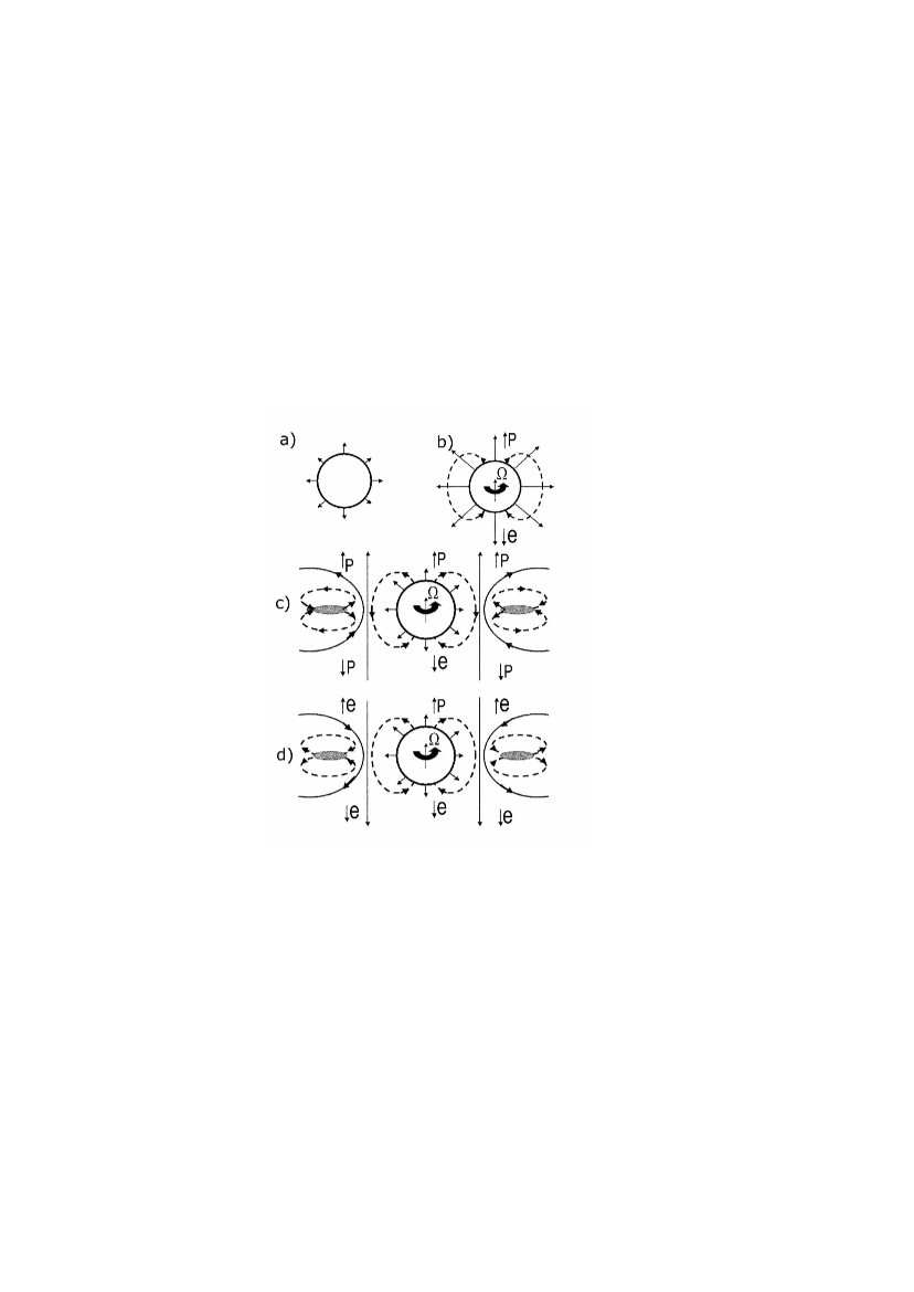
Figure 2: A schematic toy model of the WH/BH: (a) WH or BH with a radial magnetic field. (b) Same as (a), with rotation and a dipolar electric field. (c) Same as (b), with a rotating accretion disk with its dipole magnetic field and quadrupolar electric field. (d) Same as (c), with dipole magnetic and quadrupole electric fields of the opposite direction. The arrows (p) and (e) indicate the directions for proton and electron jets, respectively.

Figure 2 presents WH/BH models allowing for the possibility that they possess an evolved accretion disk with its own magnetic field (probably dipolar and substantially weaker than the field of the WH/BH themselves). This is a schematic toy model in the vacuum approximation. The presence of a radial magnetic field can be revealed by the law for the increase in the field strength ${(H\propto r^{-2})}$ and the presence of the same sign of the field on all sides. The rotation of the monopole excites a dipolar electric field, which can provide acceleration for relativistic particles. Note that the dipole electric field (in contrast to the quadruple field for a disk) accelerates electrons towards one of the poles (and protons and positrons towards the other; see Appendix 6.3). Of course such motion of electrons is possible only if there are currents providing the electro neutrality of the system. Something like this may explain the origination of one-sided jets in some sources (for example, the quasar 3C273) [18].

Actually the general picture should be much more complicated.

First of all the rarefied plasma form a complex magnetosphere around WH/BH (see [19]). In addition the presence of the accretion disk complicates the picture. In a toy model the quadrupolar electric field generates two-sided electron or proton/positron jets (depending on the sign of the quadrupole). As a result, the structure of the jets may be different:

1) electrons from the magnetic WH/BH are ejected from one pole, while protons (positrons) are ejected from the other,

2) electrons from the WH/BH and the accretion disk are ejected from one pole, while protons (positrons) from the WH/BH and electrons from the accretion disk are ejected from the other,

3) electrons from the WH/BH and protons (positrons) from the accretion disk are ejected from one pole, while protons (positrons) from the WH/BH and accretion disk are ejected from the other. The interactions between the electromagnetic fields of the WH/BH and accretion disk are likely to be very strong.

We have to remember that even in the toy model such jets are possible only under the conditions of existence of the electric currents providing the electro neutrality of the system and inducted electric field conserves.

The difference between a WH entrance and a BH may be revealed from observations indicating the absence of a horizon — a source of light falling into aWH should be observed continuously, but with a variable red, and even blue, shift. However, in this case, we must assume the tunnel is transparent. A blue shift can appear if the mass of the further WH entrance (relative to the observer) exceeds that of the closer entrance. If the tunnel is transparent and has accretion disks at both entrances, the redshift of the spectra of these disks will also be different. Thus, two different redshifts from a single source related to aWH could be distinguished.

An observed WH image may display some internal structure, whose angular size could be substantially smaller than that specified by the gravitational diameter.

In this connection, observations of the gravitationally lensed quasar Q0957+561 with the redshift ${z=1.4141}$ [20] are of great interest. The observation show that in this active galaxy exist the central compact object with mass ${3.6\cdot 10^{9}M_{\odot}}$, strong magnetic moment and without an event horizon. A specific property ofWHs, which display strong relativistic effects and also the absence of a horizon, is the possibility of periodic oscillations of a test mass relative to the throat (See TABLE 1 and Appendix 6.1). The redshift will also vary periodically. If the structure of the WH is close to the formation of the horizon, these shifts, the period, and the flux variations can be very large. We point out in this connection the quasi-periodic flux variations observed for so-called IDV sources, such as the BLLac object 0716+714 [21].

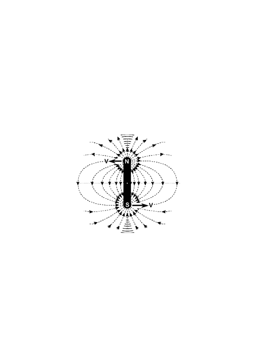
Figure 3: Schematic model of a binary system of two magnetic WHs/entrances.

When sources move along circular orbits around a WH entrance (the laws of motion see in [17] and Appendix 6.4), the flux and redshift of radiation of a compact source will also vary periodically.

Ultimately, an external observer may be able to detect some radiation at the gyrofrequencies and events related to the creation of ${e^{\pm}}$ and ${\mu^{\pm}}$ pairs (where $\mu$ designated a magnetic monopole).

Let us also consider the possibility of binary objects formed by two entrances to the same WH that interact gravitationally and electromagnetically and rotate about their common center of gravity. If the two entrances in the model with a magnetic field represent magnetic monopoles of different signs, then the binary forms a rotating magnetic dipole. Such binaries with closely-spaced entrances are also very likely to originate in the primordial scalar field, and can be preserved until the present (Fig. 3).

Let us denote: $d$ — is the distance between the WH entrances, $T$ — is the period of the circular orbit, and ${M_{\infty}}$ — is the asymptotic mass at infinity of each entrance.

As it is shown in Appendix 6.1 in our model the magnetic field ${H_{0}}$ at the throat of the WH is related with ${M_{\infty}}$:

$$H_{0}\approx\left(c^{4}/G^{3/2}\right)\,M_{\infty}^{-1}$$ (1)

Then for the circular orbit (see [17]):

$$V=\sqrt{{GM_{\infty}\over d}}\,,\quad T=\pi\sqrt{{d^{3}\over GM_{\infty}}}\,.$$ (2)

These relations are derived in the Newtonian approximation and for motion under the action of the gravitational and magnetic fields.

The intensity of magnetic-dipole ${I_{mag}}$ and gravitational ${I_{grav}}$ radiation is correspondingly [22]:

$$I_{mag}={2^{5}G^{3}M_{\infty}^{4}\over 3c^{3}d^{4}}\,,$$ (3)

$$I_{grav}={2^{9}G^{4}M_{\infty}^{5}\over 5\cdot c^{5}d^{5}}\,.$$ (4)

Gravitational radiation dominates only at very small distances ${d<(3/5)\cdot 2^{4}\cdot(GM_{\infty}/c^{2})\leq 9.6r_{0},}$ (see appendix 6.1) so that the losses of the energy and evolution of the system are determined by the magnetic-dipole radiation (3).

The characteristic time of the evolution of the system due to the radiation is ${t_{em}=|{\cal E}_{total}|/I_{mag},}$ where

$${\cal E}_{total}=-M_{\infty}V^{2}$$ (5)

Hence the system parameters preserved over time ${t_{em}}$ are no smaller than

$$d^{3}_{em}={2^{5}G^{2}M_{\infty}^{2}t_{em}\over 3c^{3}}\,,\quad T_{em}=\pi\sqrt{{2^{5}GM_{\infty}t_{em}\over 3c^{3}}}\,.$$ (6)

A rotating system of macroscopic magnetic dipole induces an electric field, which accelerate electrons and emit electromagnetic radiation along the axis of the magnetic dipole (similarly to pulsars) or even create of electron-positron pairs. Corresponding critical electric field is ${{\cal E}_{cr}=4\cdot 10^{13}.}$ Now if we specify ${t_{em}}$ equal ${t_{{}_{U}}}$ the age of the Universe ${t_{{}_{U}}\approx 13\cdot 10^{9}}$ years, we obtain the following characteristic of the system with electric field ${{\cal E}_{cr}}$ and ${t_{em}=t_{{}_{U}}}$:

$$M_{\infty}=3.2\cdot 10^{35}g\approx 160\,M_{\odot}\,,\quad d_{em}=4.2\cdot 10^{14}cm\,,\quad T_{em}=1.9\cdot 10^{8}s\approx 6\,yrs\,,\quad V_{em}\approx 70\,km/s\,.$$ (7)

All binary systems with smaller masses will generate ${e^{\pm}}$, forming two-sided jets of relativistic particles in the orbital plane, lose energy, and collapse.

TABLE 1 presents the parameters of magnetic WHs with various masses (notations see in appendix 6.1) and estimates for the intensity of magnetic-dipole radiation ${I_{mag}}$, the component separation ${d_{em}}$, the rotational period ${T_{em}}$ and velocity ${V_{em}}$ for systems preserved to the present epoch.

In this toy model binaries can be detected as strictly periodical nonthermal sources (similar to pulsars) with two jets of relativistic ${e^{\pm}}$ in the equatorial plane and a cloud of annihilating low-energy particles ${e^{\pm}}$.

The approach of the two entrances of the same magnetic WHs ends with its transformation into a BH with a mass of ${\sim M_{\infty}}$ without a magnetic field, with the radiation of the external magnetic field ${{\cal E}_{mag,\,total}\approx M_{\infty}c^{2}}$, similar to the collapse of a magnetized body [23], [24]. The electromagnetic impulse accelerates the created ${e^{\pm}}$ pairs, and may represent the basic mechanism for some type of observable $\gamma$-ray bursts. The approach of two closely spaced different WH entrances should be somewhat different: after they merge, probably one entrance or a BH is formed, with its magnetic flux equal to the sum of the original magnetic fluxes, taking into account their signs and the radiation of the difference in the flux. Thus, various merging processes could result in the formation of more massive objects, within which the entrances and magnetic fluxes from many tunnels are combined.

3 WORMHOLES AND THE MULTI-UNIVERSE

As we mentioned in section 1, there is a hypothesis that a wormholes can connect different Universes in the model of multi-universe (see fig. 1).

In this section briefly consider various aspects of such a possibility. Let us consider the possible observational differences of the two cases:

(a) both entrances of the wormhole are in our Universe and

(b) one entrance is in our Universe and another entrance is in another Universe.
In case (a) both entrances probably were formed in the very early quantum period of the existence of our Universe. It means that both of them were formed practically at the same moment of time of an external observer which is practically at rest with respect to the entrances. If during the subsequent evolution of the Universe there was not great relative velocity of the motion of the entrances and if there was not great difference in gravitational potential in their surrounding then in our epoch, time near each entrance corresponds to the same cosmological time of our epoch.

Hence an observer looking through the throat of the wormhole sees our Universe at present epoch (but another regions of it). The radiation from the wormhole would be provided mainly by the processes near both entrances rather then the cosmic microwave background which is quite weak.

In case (b) situation may be quite different. In principle the physics in our and other universe can be absolutely different and in principle we can observe it. But even if we suppose that another Universe is similar to our one there is not probably any correlation in times in these universes. Thus in this case we can see through the wormhole any epoch in the evolution of the Hot Universe: (1) very early one, or (2) close to our epoch, or (3) very late epoch.

In case (1) we would see the epoch which corresponds to very hot background radiation. The flux of the radiation through the wormhole into our Universe would rapid decrease the mass and the size of the entrance in our Universe and would lead to rapid conversion of it into (a) black hole or into a naked singularity.

The dynamics of space-time of a wormhole in the case of a strong flux of matter through it needs a special investigation and we will discuss it in a separate paper.

Here we want to mention that such an instability of a wormhole with respect to flux of energy brought it may be very important also in the case (a) at the very early epoch if there is not a good balance of the contrary fluxes of radiation in both entrances.

Case (2) would be similar to the case (a) from the point of view of observations.

In case (3) we would see a very cold Universe without any significant radiation from it.

It is worthy of consideration the following problem. The entrance, in which the flux of radiation is falling down, would increase in mass and in size. As we mentioned above the opposite entrance would shrink down and eventually probably would disappear.

The question arises: what does an observer near first entrance see when the second entrance disappears? This question is a part of the problem about the evolution of the wormhole in the case of a strong flux of energy through it and will be considered in a separate paper.

4 CONCLUSION

In this paper we propose to analyze the possibility of identifying a new type of primordial cosmological objects — WHs entrances, or BHs formed from WHs — among known Galactic and extragalactic objects that are usually identified with neutron stars or stellar-mass and super massive BHs. The implied presence of a strong radial magnetic field (the ”hedgehog”  model [24], [25], [26]) is very important, and can, together with rotation, bring about the generation of (one- and two-sided) relativistic jets. WH models suggest the specific properties of such objects related to the absence of a horizon, which makes it possible to observe sources of radiation at any point of the tunnel, if the tunnel medium is transparent. A certain behavior is expected for the variations of the spectrum, flux, and polarization of the source of radiating objects making periodic oscillations relative to a WH throat could be detected.

The observer structures of the sources that could be related To WHs entrances (or BHs) with a radial magnetic field could be studied with microarcsecond or better angular resolution, as is proposed in the ”Radioastron”  and ”Millimetron”  space-VLBI experiments [27], [28].

It may be possible to detect sources associated with binary WHs entrances, which form systems with strong magnetic-dipole radiation and the ejection of relativistic ${e^{\pm}}$. The final stage in the evolution of such systems is the formation of a BH, accompanied by strong electromagnetic impulses.

Note also that the possible existence of WHs with strong magnetic fields suggests that theoretically predicted elementary magnetic monopoles [27], [28] could have merged with these objects in the course of their cosmological evolution.

Another direction for future studies is related to spectral and polarization monitoring of these sources.

The detection of tunnels will open the way to studies of the entire Multiverse.

In the Appendixes we consider the explicit mathematical models of the WHs with magnetic field which are the theoretical basis of our hypothesis.

5 ACKNOWLEDGEMENTS

This work was supported by the Russian Foundation for Basic Research (project numbers: ${05-02-17377}$, ${05-02-16302-a}$, ${04-02-16987-a}$, ${04-02-17257-a}$) and the Program in Support of Leading Scientific Schools of the Russian Federation ${(NSH-1653.2003.2)}$ and program ”stellar evolution”.

The authors are grateful to S.P. Gavrilov [29], B.V. Komberg, M.B. Mensky, D.I. Novikov, V.I. Ritus, and A.E. Shabat for useful discussions and comments.

6 APPENDIXES

6.1 Spherically symmetrical wormhole with radial magnetic field

The metric of a spherical WH can be presented in the form (see [30]):

$$ds^{2}=e^{2\phi(r)}\,dt^{2}-{dr^{2}\over 1-b(r)/r}-r^{2}\,d\Omega^{2}\,,$$ (8)

where $r$ is the radial coordinate, ${\varphi(r)}$ the so-called redshift function, and ${b(r)}$ the form function. The WH neck corresponds to the minimum ${r=r_{0}=b(r_{0})}$ and ${b_{(r_{0})}\leq 1}$. The presence of a horizon corresponds to the condition ${\varphi\to-\infty}$ or ${e^{\varphi}\to 0}$; for WH $\varphi$ must be finite everywhere.

Let us introduce the mass ${M(r)}$ of the WH for an external observer:

$$M(r)=M_{0}+\int\limits_{r_{0}}^{r}4\pi\varepsilon r^{2}\,dr\,,$$ (9)

where ${M_{0}=r_{0}/2}$ and ${\varepsilon(r)}$ — is the energy density. For convenience in graphical representation and calculations, we introduce the variable ${x=r_{0}/r}$. The entire interval ${r_{0}\leq r<\infty}$ will then be transformed into ${0<x\leq 1}$, and we obtain the equation for a static WH:

$$\begin{array}[]{lll}8\pi\varepsilon r_{0}^{2}=-b^{\prime}x^{4}/r_{0}\,,\\ \\ 8\pi p_{\parallel}r_{0}^{2}=-bx^{3}/r_{0}-2x^{3}(1-bx/r_{0})\phi^{\prime}\,,\\ \\ 8\pi p_{\perp}r_{0}^{2}=(1-bx/r_{0})\left[x^{4}\phi^{\prime\prime}+x^{3}\phi^{\prime}+x^{4}(\phi^{\prime})^{2}\right]+0.5x^{3}(xb^{\prime}+b)(1-x\phi^{\prime})/r_{0}\,.\end{array}$$ (10)

where the derivatives are taken with respect to $x$. It was shown in [31] that, in a spherically symmetrical WH with ${w_{\parallel}=const}$ and ${w_{\perp}=const}$, an inequality specifying possible equations of state and their anisotropy must be satisfied:

$$-2w_{\perp}<w_{\parallel}<-1$$ (11)

The left-hand side of the inequality specifies the finiteness of the WH mass as ${r\to\infty}$, while the right-hand side indicates the absence of a horizon.

It is of great interest that condition (11) is ”almost”  satisfied for a magnetic (or electric) field. If the field is in the $r$ direction, the energy-momentum tensor specifies the equation of state

$$w_{\parallel}=-1\,,\quad w_{\perp}=1\,,\quad\varepsilon=(H^{2}+E^{2})/(8\pi)\,,$$ (12)

which satisfies the conditions (11) for a WH to within a small negative increment in ${w_{\parallel}}$.

In [32], a model for a phantom-matter WH with an anisotropic equation of state is considered:

$$1+\delta=-p_{\parallel}/\varepsilon=p_{\perp}/\varepsilon\,,$$ (13)

and it is shown that even an arbitrarily small $\delta$ is sufficient for a WH to exist.

Let us denote ${x_{h}=r_{0}/r_{h}>1}$ to be the ratio of the radii of the WH throat and the horizon of the corresponding Reissner-Nordstrem black hole (BH) [33] with magnetic charge ${Q=r_{h}}$ (see [17]). $\varepsilon$ is specified by the relation

$$\varepsilon=\varepsilon_{0}\,x^{4}\,\left[(x_{h}-1)/(x_{h}-x)\right]^{\delta}\,,\quad\varepsilon_{0}=1/(8\pi r_{0}^{2}(1+\delta))\,.$$ (14)

For an observer far from the throat, the WH mass ${M_{\infty}}$ is in the interval

$$M_{0}\leq M_{\infty}\leq 2M_{0}$$ (15)

The left-hand side of the inequality follows from (9), and the right-hand side from (14).

In this connection, it may be concluded that the electromagnetic (EM) field may be an appreciable or even predominant part of the WH. Let us consider three types of models:

(1) an EM field is the main component of the WH matter. In addition a small amount of the phantom energy is necessary to provide conditions above,

(2) an EM field plus phantom energy with an isotropic equation of state,

(3) an EM field plus phantom matter with an anisotropic (vector-type) equation of state.

Common to all three models is the assumption that the WH is penetrated by an initial magnetic field, which should display a radial structure for an external observer in the spherically symmetrical case; i.e., it should be correspond to a macroscopic magnetic monopole (${r\to\infty}$, ${H\propto r^{-2}}$, and ${\varepsilon_{{}_{H}}\propto r^{-4}}$). The two entrances to the WH should have opposite signs of the magnetic field.

In model 1 there is the magnetic field plus a small amount of phantom energy or phantom matter. Under real conditions, this model is specified by a strong magnetic field. The fact that $\delta$ is small indicates that the configuration is close to a BH. The accretion of normal matter onto the WH entrance results in the growth of ${w_{\parallel}}$, and the condition of the absence of a horizon can be violated (the right-hand side of (11)). The WH entrance can then turn into a BH with the radial magnetic field. The opposite is also true: the accretion of phantom energy makes the WH more different from a BH [34]. Overall, model 1 is close to a BH with an extremely strong magnetic field [35], which, however, displays a monopole rather than a dipole structure.

TABLE 1 presents the parameters for the throats of magnetic WHs with various masses ${M_{0}}$. We can use (14) (and the constants $c$ and $G$) to derive expressions for $r_{0}$, $H_{0}$, $\rho_{0}$ (the mass density), ${\nu_{{}_{G}}}$ (the frequency of oscillations with a small amplitude for a sample particle), and ${\nu_{{}_{H}}}$ (the gyrofrequency) in the throat and its rest frame; $\nu_{c}$ is the frequency of revolution along the lower stable circular orbit for an external observer. Then,

$$\begin{array}[]{l}r_{0}=(G/c^{2})\cdot M_{\infty}\,;\\ H_{0}=(c^{4})/(G^{3/2})\cdot M_{\infty}^{-1}\,;\\ \rho_{0}=(c^{6})/(8\pi G^{3})\cdot M_{\infty}^{-2}\,;\\ \nu_{{}_{G}}=(c^{3})/(2\sqrt{2}\pi G)\cdot M_{\infty}^{-1}\,;\\ \nu_{{}_{H}}=(ec^{3})/(2\pi m_{e}G^{3/2})\cdot M_{\infty}^{-1}\,;\\ \nu_{c}=(\sqrt{3}c^{3})/(32\pi G)\cdot M_{\infty}^{-1}=\sqrt{(3/128)}\cdot\nu_{{}_{G}}\,.\end{array}$$ (16)

TABLE 1

Parameters of the throats of magnetic WHs with various masses^∗:

$M_{\infty}=2M_{0}$	$r_{0}$, cm	$H_{0}$, Gs	$\rho(r_{0})$, g/cm3	$\nu_{{}_{G}}$, Hz	$\nu_{{}_{H}}$, Hz	$\nu_{c}$, Hz
$6\cdot 10^{42}$ g$=3\cdot 10^{9}M_{\odot}$	$4.5\cdot 10^{14}$	$7.8\cdot 10^{9}$	$2.7\cdot 10^{-3}$	$7.6\cdot 10^{-6}$	$2.2\cdot 10^{16}$	$1.16\cdot 10^{-6}$
(Quasar)				(1.5 Days)		($9.8$ Days)
$10^{39}$ g$=5\cdot 10^{5}M_{\odot}$	$7.4\cdot 10^{10}$	$4.4\cdot 10^{13}$	$9.7\cdot 10^{4}$	$0.045$	$1.3\cdot 10^{20}$	$6.9\cdot 10^{-3}$
($e^{\pm}$ pair creation)				($22$ s)		($2.4$ min)
$2\cdot 10^{33}$ g$=M_{\odot}$	$1.5\cdot 10^{5}$	$2.3\cdot 10^{19}$	$2.4\cdot 10^{16}$	$2.3\cdot 10^{4}$	$6.6\cdot 10^{25}$	$3.5\cdot 10^{3}$
(Sun)
$6\cdot 10^{27}$ g$=M_{\oplus}$	$0.45$	$7.8\cdot 10^{24}$	$2.7\cdot 10^{27}$	$7.6\cdot 10^{9}$	$2.2\cdot 10^{31}$	$1.16\cdot 10^{9}$
(Earth)
$5\cdot 10^{10}$ g	$3.5\cdot 10^{-18}$	$10^{42}$	$4.4\cdot 10^{61}$	$9.7\cdot 10^{26}$	$2.7\cdot 10^{48}$	$1.5\cdot 10^{26}$
(positronium)
$1.8\cdot 10^{3}$ g	$1.3\cdot 10{-25}$	$2.6\cdot 10^{49}$	$3\cdot 10^{76}$	$2.6\cdot 10^{34}$	$7.3\cdot 10^{55}$	$4\cdot 10^{33}$
($\mu^{\pm}$ pair creation)
$2\cdot 10^{-5}$ g	$1.5\cdot 10^{-33}$	$2.3\cdot 10^{57}$	$2.4\cdot 10^{92}$	$2.3\cdot 10^{42}$	$6.6\cdot 10^{63}$	$3.5\cdot 10^{41}$
(Planck mass)

Binary WH entrances^∗:

${M_{\infty}}$	${I_{mag}}$, erg/s	${d_{em}}$, cm	${T_{em}}$, s	${V_{em}}$, km/s
$6\cdot 10^{42}$ g$\approx 3\cdot 10^{9}M_{\odot}$	$7.0\cdot 10^{40}$	$3.0\cdot 10^{19}$	$8.2\cdot 10^{11}$	${1100}$
(quasar)
$3.2\cdot 10^{35}$ g$\approx 160\cdot M_{\odot}$	$4.0\cdot 10^{31}$	$4.2\cdot 10^{14}$	$1.9\cdot 10^{8}$	${70}$
($e^{\pm}$ pair creation)
$2\cdot 10^{33}$ g$=M_{\odot}$	$4.6\cdot 10^{28}$	$1.4\cdot 10^{13}$	$1.5\cdot 10^{7}$	${30}$
(Sun)
$9\cdot 10^{18}$ g ∗∗	$3.4\cdot 10^{9}$	$3.8\cdot 10^{3}$	$1$	${120}$ m/s
(Micropulsar)
$1.8\cdot 10^{3}$ g	$4.0\cdot 10^{-12}$	$1.3\cdot 10^{-7}$	$1.4\cdot 10^{-8}$	${30}$ cm/s
($\mu^{\pm}$ pair creation)
$2.2\cdot 10^{-5}$ g	$1.1\cdot 10^{-22}$	$7.0\cdot 10^{-13}$	$1.6\cdot 10^{-12}$	${1.4}$ cm/s
(Planck mass)

^∗See appendix 6.1.

^∗∗Binary WH with orbital period 1 s.

In TABLE 1, WH parameters are estimated for quasar cores, as well as for objects with the field (and corresponding WH mass) critical for the creation of electron-positron pairs, with masses of the order of the Sun’s and the Earth’s, with the magnetic field (and WH mass) critical for stability of the positronium atom, with the magnetic field (and WH mass) critical for the creation of monopole-anti-monopole pairs, and with the Planck mass.

The magnetic field for a model described by (14) with a small $\delta$ will be

$$H\approx M_{\infty}\sqrt{G}/r^{2}$$ (17)

Assuming that the electric field is small, the constraint associated with the creation of electron-positron pairs is removed (although we present it in the TABLE 1 for the limiting case). This field, ${H=m^{2}_{e}c^{3}/\mu_{{}_{H}}\approx 4.4\cdot 10^{13}\,G}$, specifies specific conditions related to the fact that, at large fields, the Landau excitation level exceeds the electron rest energy. The positronium atom becomes stable in fields above ${10^{42}\,G}$, and the medium becomes filled with such atoms created from the vacuum [36], [37]. In magnetic fields stronger than the critical value ${H_{max}}$, a vacuum puncture and the creation of monopole pairs occur [38]-[41]. If the mass of a stable, colorless monopole [42]-[44] is ${m_{\mu}\sim 10^{16}\,GeV\sim 10^{-8}g}$ and the magnetic charge ${\mu=(3/2)\hbar c/e\sim 10^{-7}}$, then ${H_{max}=m^{2}_{\mu}c^{3}/\mu\hbar\approx 2.6\cdot 10^{49}\,G}$, and, according to (15), the maximum mass of a magnetic WH with this field in its throat is ${M_{\infty}\approx 1.8\,kg}$. The created monopoles will be ejected from the WH, decreasing its mass. It is not obvious whether such small WHs are stable against other quantum processes, and the minimum mass of the WH may turn out to be substantially higher than $1.8\,kg$. The lower limit for the mass of a WH with a composite constitution is obviously even lower. Note also that the absence of a horizon for the WH results in the absence of evaporation (Hawking radiation). Therefore, primordial low-mass WHs could be preserved until the current epoch, unlike primordial BHs (for which the lower limit for the mass is ${\sim 10^{15}g}$).

Model 2 corresponds to the case of phantom energy, similar to that used in cosmological models. Since the equation of state is isotropic, phantom energy alone cannot satisfy the left-hand side of (11), and a larger fraction of magnetic field is needed. Let us denote the fraction of the magnetic-energy density ${\eta_{{}_{H}}=\varepsilon_{{}_{H}}/\varepsilon}$ and the fraction of the phantom-energy density ${\eta_{w}=\varepsilon_{w}/\varepsilon}$, ${\varepsilon=\varepsilon_{{}_{H}}+\varepsilon_{w}}$. If the pressure is ${p_{w}=w\varepsilon_{w}}$ and ${\eta_{{}_{H}}+\eta_{w}=1}$ for the phantom matter, then ${p_{\parallel}=-\varepsilon_{{}_{H}}+w\varepsilon_{w}}$, ${p_{\perp}=\varepsilon_{{}_{H}}+w\varepsilon_{w}}$, and it follows from (11) with conditions ${w_{\parallel}=const}$ and ${w_{\perp}=const}$ that

$$3w/(3w-1)<\eta_{{}_{H}}<1\,,\quad 0<\eta_{w}<1/(1-3w)$$ (18)

As ${w\to-1}$, the fractions of the magnetic and phantom energies are ${0.75<\eta_{{}_{H}}<1}$ and ${0<\eta_{w}<0.25}$. As ${w\to-\infty}$, ${\eta_{{}_{H}}\to 1}$, and ${\eta_{w}\to 0}$. Thus, for an electromagnetic WH, it is necessary and sufficient to include an arbitrarily small fraction of phantom energy with an isotropic equation of state, with w arbitrarily close, but smaller than ${-1}$.

Figure 4 presents the results of calculating equations (10) for all three models. It shows the dependence of the fractions of ${\eta_{{}_{H}}}$, ${\eta_{w}}$, and ${\eta_{{}_{CDM}}}$ on ${x=r_{0}/r}$ for the models with a radial magnetic field, phantom energy (with ${w\to-1}$), and ordinary matter with ”zero”  pressure (the fraction ${\eta_{{}_{CDM}}}$). The limiting conditions are ${\eta_{{}_{H}}=\eta_{w}=0.5}$ in the throat, ${\eta_{w}\to\eta_{{}_{CDM}}\to 0}$ for ${x\to 0\,\,(r\to\infty)}$. Here, in the three-component model, unlike (13), ${w_{\parallel}}$ and ${w_{\perp}}$ depend on $r$.

Model 3 can provide any relation between the magnetic and phantom matter density, while, according to [32], $\delta$ can be arbitrarily small.

We want to emphasize that the relations between $p$ and $\varepsilon$ correspond to the static state and we do not consider the static state and we do not consider the dynamics. Particularly we do not consider the problem of stability of wormholes.

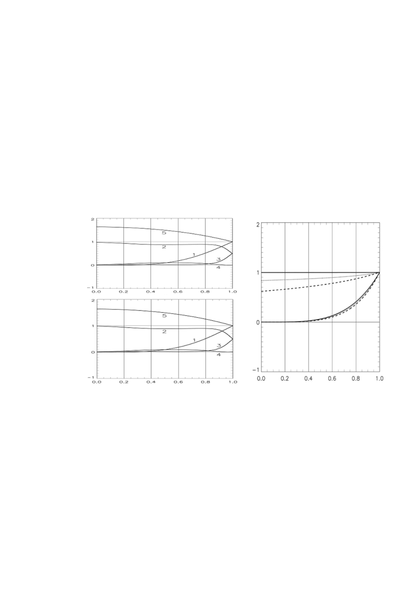
Figure 4: Basic model parameters as functions WH of ${x=r_{0}/r}$. The top-left plots shows the three-component model with ${w_{{}_{H}}=1,\,\,w=-1}$, and ${\eta_{{}_{H}}(1)=\eta_{w}(1)=0.5}$. The dependences are indicated for (1) the total density in a throat, (2) the magnetic-field density from the total density, (3) the phantom-energy density, (4) the ordinary-matter density, and (5) the total density in a throat not divided by ${x^{4}}$ (this characterizes the difference of distribution for the density from that for a magnetic monopole). The bottom-left plots show the same dependences for the three-component model for ${w_{{}_{H}}=1,\,\,w=1.02}$, and ${\eta_{{}_{H}}(1)=\eta_{w}(1)=0.5}$. The right-hand-side plots show the model for a WH supported mainly by a magnetic field (or by phantom matter with the same $\delta$). The three lower curves represent the dependence of the fractional density on the density in the throat ${\eta=\varepsilon/\varepsilon_{0}}$ for ${\delta=0.5}$ (dashed), ${\delta=0.1}$ (dotted), and ${\delta=0.001}$ (solid); the three upper curves correspond to the lower curves with ${\eta/x^{4}}$ (characterizing the difference of the structure from a monopole). As ${\delta\to 0\,\,\eta/x^{4}\to 1}$. About notations see the end of section 6.1.

6.2 DIPOLAR ELECTRIC FIELD INDUCED IN A WH

In the case of a rotating WH with a magnetic field, the electric field that is induced should display a dipolar structure, due to the monopolar WH magnetic field.

Characteristic estimates for the induced WH electric field can be obtained from the exact solution corresponding to a BH [19]. Making the substitution ”electricity $\longleftrightarrow$ magnetism”  in the solution, we obtain for the electric field:

$$\vec{E}(r,\theta)\approx H(r_{h})\cdot{a\cdot r_{h}^{2}\over r^{3}}\cdot\left(2\,\cos\theta\cdot\vec{e}_{r}+\sin\theta\cdot\vec{e}_{\theta}\right)$$ (19)

Observationally, the existence of such a field in the vacuum approximation in a toy model will result in the ejection of electrons from one of the poles and protons from the other. Standard Blandford-Znajek type [45] hydrodynamical models or models with a quadrupolar electric field predict two-sided jets for BHs. In addition, even in the case of slow rotation, such a jet should display a higher energy, since its acceleration results from a larger electric potential then in the case of a BH: ${\varphi_{e}\sim H(r_{0})a}$ for a WH, while ${\varphi_{e}\sim H(r_{h})a^{2}/r_{h}}$ for a BH, where $a$ is the rotation parameter in the Kerr metric.

6.3 OBSERVATIONS OF BODY OSCILLATING THROUGH A WH THROAT

Oscillations of bodies in the vicinity of a WH throat (radial orbits) could give rise to a peculiar observational phenomenon. Signals from such sources detected by an external observer will display a characteristic periodicity in their spectra. All objects (stars, BHs) other than WHs absorb bodies falling onto them irrecoverably. Periodic radial oscillations are a characteristic feature of WHs.

For simplicity, let us consider a test body with zero angular momentum. We will solve the equations of motion using the Hamilton-Jacobi method in a curved space [22].

We then obtain for the velocity of the body:

$${\partial r\over\partial t}=\pm\exp(\phi)\cdot\sqrt{\left[1-b/r\right]\cdot\left[1-\exp(2\phi)\cdot(m_{0}/E_{0})^{2}\right]}$$ (20)

Here, ${m_{0}}$ and ${E_{0}}$ are the rest mass and total energy of the body.

Expression (20) does not correspond to the physical velocity of the body, since $r$ is not the physical radial coordinate. The physical velocity of the body along the radius, ${\dot{l}}$ (with respect to time $t$) is

$$\dot{l}=\pm\exp(\phi)\cdot\sqrt{1-\exp(2\phi)\cdot(m_{0}/E_{0})^{2}}$$ (21)

The redshift of a signal radiated by the body is specified by the following two factors.

(1) The Doppler shift due to the motion of the source yields the factor ${\sqrt{1-v^{2}}/(1\pm v)}$, where ${v=\dot{r}\sqrt{|g_{rr}/g_{tt}|}}$ is the physical velocity of the body in its proper time (here, the signs $\pm$ correspond to motion of the body from and toward the observer).

(2) The gravitational redshift yields the factor ${\exp\varphi}$.

Thus, the frequency of the signal received by a distant observer will be given by the expression

$$\nu=\nu_{0}\cdot{\exp(2\phi)\cdot(m_{0}/E_{0})\over 1\pm\sqrt{1-\exp(2\phi)\cdot(m_{0}/E_{0})^{2}}}$$ (22)

Here, ${\nu_{0}}$ is the frequency of the signal measured on the moving body. It follows that, unlike a BH horizon, the frequency of the signal in the WH throat does not become equal to zero for a distant observer.

In order to find the time dependence of the redshift ${\nu/\nu_{0}}$ of the body for an external observer, time ${\Delta t}$ for the light to propagate from point $r$ to point ${r_{max}}$ of the body must be added to time $t$. Figure 5 presents these dependencies.

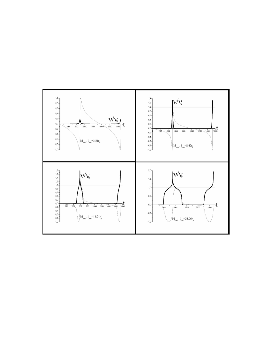
Figure 5: Time dependences of the frequency shift ${\nu/\nu_{0}}$ (thick curve) and physical radial coordinate ${l/l_{max}}$ (thin curve); time $t$ is in units of ${r_{h}/c}$. The graphs are plotted for ${\delta=0.001}$.

For extremely small amplitudes ${(r_{1}-r_{0})}$, the test-body oscillations become harmonic. This situation is reached when the following inequality is satisfied:

$$r-r_{0}\leq r_{1}-r_{0}<<r_{0}-r_{h}\,,\qquad 1-x\leq 1-x_{1}<<x_{h}-1\,,$$ (23)

where $x_{1}=r_{0}/r_{1}$. In this case, in the vicinity of the points where the body stops, the components of its velocity ${\dot{r}}$ (20) can be expanded in a series in ${1-x}$ (or ${x-x_{1}}$). Restricting the expansion to the main terms yields

$$e^{\phi}\approx(x_{h}-1)\,,\quad(1-{b\over r})\approx(x_{h}-1)(1-x)\,,\quad 1-e^{2\phi}(m_{0}/E_{0})^{2}\approx{2(x-x_{1})\over x_{h}-1}\,.$$ (24)

Hence,

$$(\dot{r})^{2}\approx 2(x_{h}-1)^{2}(1-x)(x-x_{1})\,,\quad r_{h}\ddot{r}=\dot{r}{\partial\dot{r}\over\partial x}={1\over 2}{\partial(\dot{r})^{2}\over\partial x}\,,\quad(1-x)\,\ddot{}=-\omega_{0}^{2}(1-x)\,,$$ (25)

where ${w_{0}=\sqrt{2}(x_{h}-1)/r_{h}}$. This is the equation for harmonic oscillations with the body stopping at ${x=1}$ and ${x=x_{1}}$; therefore, the period of these oscillations measured by an external observer will be

$$T_{1}={\sqrt{2}\pi r_{h}\over c(x_{h}-1)}.$$ (26)

In this case, the oscillations of the physical coordinate $l$ are also harmonic, as follows from (21) and (24). The body oscillates from ${-l_{1}}$ to ${+l_{1}}$; the condition that ${l_{1}}$ be small, corresponding to (20), is ${l_{1}<<r_{h}}$ (thus, in these coordinates, the amplitude does not have to be extremely small).

The oscillations of coordinate l have a period that is twice this value ${(T_{2}=2T_{1})}$.

6.4 CIRCULAR ORBIT AROUND A WH

The difference of the metric of the limiting Reisner-Nordstrem and our model of the WH is negligible at ${r=2r_{h}}$ (or more). Thus all conclusions about circular orbit around a WH are the same as in the limiting Reisner-Nordstrem geometry at the corresponding distances.

We obtain (see [46],[47]) for the period at the circular orbit with respect to time $t$:

$$\tau=\int\limits_{0}^{2\pi}{d\varphi\over\dot{\varphi}}={2\pi r^{2}E_{0}/L\over c^{2}(1-r_{h}/r)^{2}}\,,$$ (27)

where ${E_{0}}$ — is the energy and $L$ — is the angular momentum.

Hence, the periods of the last stable and unstable circular orbits (according to a distant observer) are

$$\tau(4r_{h})={32\pi r_{h}\over\sqrt{3}c}\,,\quad\tau(2r_{h})={8\pi r_{h}\over c}\,.$$ (28)

References

- [1] J. A. Wheeler, Phys. Rev. 97, 511 (1955).
- [2] C. W. Misner and J. A. Wheeler, Ann. Phys. (N.Y.) 2, 525 (1957).
- [3] J. A. Wheeler, Ann. Phys. (N.Y.) 2, 604 (1957).
- [4] A. Vilenkin, Phys. Rev. D 27, 2848 (1983).
- [5] A. Linde, Phys. Lett. B 175, 395 (1986).
- [6] S. W. Hawking, Black Holes and the Structure of the Universe, Eds. by C. Teitelboim and J. Zanelli (World Sci., Singapore, 2000), p. 23.
- [7] M. Visser, Lorential Wormholes: from Einstein to Hawking (Springer, AIP, 1996).
- [8] F. S. N. Lobo, Phys. Rev. D 71, 084011, (2005).
- [9] H. Shinkai and S. A. Hayward, Phys. Rev. D 66, 4005, (2002).
- [10] F. Rahaman, M. Kalam, M. Sarker, and K. Gayen, gr-qc/0512075, (2005).
- [11] P. K. F. Kuhfittig, gr-qc/0512027, (2005).
- [12] F. S. N. Lobo, gr-qc/0506001 (2005).
- [13] M. Visser, S. Kar, and N. Dadhich, gr-qc/0301003, (2003).
- [14] F. Rahaman, at al, gr-qc/0607061, (2006).
- [15] H. K. Jassal, J. S. Bagla, and T. Padmanabhan, Phys. Rev. D 72, 103503, (2005).
- [16] C. Armendariz-Picon, gr-qc/0201027, (2002).
- [17] N. S. Kardashev, I. D. Novikov, and A. A. Shatskiy, Astronomy Reports, Vol.50, N8, pp. 601-611, (2006) [published in Astronomicheski’i Zhurnal, (RUS), 2006, Vol.83, N8, pp. 675-686].
- [18] L. Stawarz, Astrophys. J. 613, 119, (2004).
- [19] Black Holes: the Membrane Paradigm, Ed. by K. S. Thorne, R. H. Price, and D. A. Macdonald (Yale Univ. Press, New Haven, 1986, Mir, Moscow, 1988).
- [20] R. E. Schild, D. J. Leiter, and L. Robertson, astro-ph/0505518, (2005).
- [21] L. Ostorero, S. J. Wagner, J. Gracia, et al., astro-ph/0602237, (2006).
- [22] L. D. Landau and E. M. Lifshitz, Course of Theoretical Physics, Vol. 2: The Classical Theory of Fields (Nauka, Moscow, 1995; Pergamon, Oxford, 1975).
- [23] V. L. Ginzburg and L. M. Ozernoi, Zh. Eksp. Teor. Fiz. 47, 1030 (1964) [Sov. Phys. JETP 20, 689, (1964)].
- [24] I.D. Novikov, Astron. Tsirk., N290, (1964).
- [25] N. S. Kardashev, Epilogue to the Russian Eddition of the Monograph by G.P. Burbidge and E.M. Burbidge ”Quasars”, (Mir, Moscow, 1969) [in Russian].
- [26] Yu. A. Kovalev and Yu. Yu. Kovalev, Publ. Astron. Soc. Jpn. 52, 1027, (2000).
- [27] Project ”Radioastron”, http://www.asc.rssi.ru/radioastron/description/intro_eng.htm.
- [28] Project ”Millimetron”, http://www.asc.rssi.ru/millimetron/millim_eng.htm.
- [29] S. P. Gavrilov, hep-th/0510093, (2005).
- [30] M. Morris and K. S. Thorne, Am. J. Phys. 56, 395, (1988).
- [31] A. A. Shatskiy, Astron. Zh. 81, 579, (2004) [Astron. Rep. 48, 525, (2004)].
- [32] A. A. Shatskiy, Astron. Zh. (2006, in press).
- [33] C.W. Misner, K. S. Thorne, and J. A. Wheeler, it Gravitation (Freeman, San Francisco, 1973; Mir, Moscow, 1977), Vol. 3.
- [34] P. F. Gonzalez-Diaz, astro-ph/0510771, (2005).
- [35] N. S. Kardashev, Mon. Not. R. Astron. Soc. 276, 515, (1995).
- [36] A. E. Shabad and V. V.Usov, hep-th/0512236, (2005).
- [37] A. E. Shabad and V. V. Usov, astro-ph/0601542, (2006).
- [38] M. Bander and H. R. Rubinstein, Phys. Lett. B 280, 121, (1992).
- [39] M. Bander and H. R. Rubinstein, Phys. Lett. B 289, 385, (1992).
- [40] R. C. Duncan, astro-ph/0002442, (2000).
- [41] Qiu-He Peng and Chih-Kang Chou, Astrophys. J. 551, L23, (2001).
- [42] G. Hooft, Nucl. Phys. B 79, 276, (1974).
- [43] A.M. Polyakov, Zh. Eksp. Teor. Fiz. 20, 194, (1974).
- [44] T.W. Kibble, J. Phys. A 9, 1387, (1976).
- [45] R. D. Blandford and R. L. Znajek, Mon. Not. R. Astron. Soc. 179, 433, (1977).
- [46] V. P. Frolov and I. D. Novikov, Black Hole Physics. Basic Concepts and New Developments (Kluwer, 1998).
- [47] B. Carr, astro-ph/0511743, (2005).