Dynamical behavior of generic quintessence potentials: constraints on key dark energy observables

Abstract

We perform a comprehensive study of a class of dark energy models – scalar field models where the effective potential can be described by a polynomial series – exploring their dynamical behavior using the method of flow equations that has previously been applied to inflationary models. Using supernova, baryon oscillation, CMB and Hubble constant data, and an implicit theoretical prior imposed by the scalar field dynamics, we find that the $\Lambda$CDM model provides an excellent fit to the data. Constraints on the generic scalar field potential parameters are presented, along with the reconstructed $w(z)$ histories consistent with the data and the theoretical prior. We propose and pursue computationally feasible algorithms to obtain estimates of the principal components of the equation of state, as well as parameters $w_{0}$ and $w_{a}$. Further, we use the Monte Carlo Markov Chain machinery to simulate future data based on the Joint Dark Energy Mission, Planck and baryon acoustic oscillation surveys and find that the inverse area figure of merit improves nearly by an order of magnitude. Therefore, most scalar field models that are currently consistent with data can be potentially ruled out by future experiments. We also comment on the classification of dark energy models into “thawing’” and “freezing” in light of the more diverse evolution histories allowed by this general class of potentials.

I Introduction

Is the universe accelerating because it is dominated by vacuum energy? The answer to this question has become a holy grail of cosmology; in addition to the increasing improvements in existing constraints Perlmutter et al. (1999); Riess et al. (1998); Knop et al. (2003); Riess et al. (2004); Astier et al. (2006), there are multiple ambitious experimental efforts currently planned to help find the answer. Vacuum energy would be spatially homogeneous and time-invariant, possessing a dark energy equation of state, $w\equiv p_{\rm DE}/\rho_{\rm DE}$, equal to $-1$ identically and at all times. Finding robust evidence for a deviation from this prediction would be tremendously important and would suggest yet another cosmological mystery: it would indicate that dark energy is more complicated than the simplest model, Einstein’s cosmological constant.

Mapping out the history of the equation of state of DE (or dark energy density), and in particular any variation in redshift of $w(z)$, is therefore one of the fundamental goals in cosmology. The simplest way to do this is to measure a single parameter that describes the time-dependence of $w(z)$, such as its derivative (e.g. Cooray and Huterer (1999); Linder (2003); Corasaniti and Copeland (2003); Hannestad and Mortsell (2004)), while the most general approach is to directly reconstruct $w(z)$ from the distance-redshift or expansion rate-redshift data Huterer and Turner (1999); Nakamura and Chiba (1999); Starobinsky (1998). With any given test, a difficult question arises: if we measure that the equation of state at some pivot redshift is consistent with $-1$ with some error, is it worth spending a large amount of time and resources in measuring the temporal variation of $w$ — which, one could naively guess, would then be small or zero in any realistic model of dark energy?

In this paper we address the following question: given the current constraints on the equation of state of dark energy that are increasingly tightening around the $\Lambda$CDM value of $-1$, and assuming a well-defined class of models that allows diverse behavior in the dark energy sector, is it worth pursuing better and more expensive cosmological probes in hope of detecting any deviation from the $\Lambda$CDM value? Our analysis differs from a large body of previous work in that we approach the question in a very general way. Instead of considering very specific examples of DE models (say, specific power law scalar field potentials), we encompass all models within a prescribed framework, constrain this entire class with the currently available data, and address how future improvements upon these constraints will affect our ability to test the $\Lambda$CDM paradigm for dark energy. To perform these tasks, we use the formalism of dynamical trajectories in model parameter space that was previously applied to slow-roll inflation models.

We make no attempt to study the individual or comparative merits of specific cosmological probes; nor do we consider optimal survey design for any particular probe. Such studies have been carried out by various authors in the past (e.g., Eisenstein et al. (1999); Huterer and Turner (2001); Weller and Albrecht (2002, 2001); Maor et al. (2002); Kujat et al. (2002); Bassett et al. (2004); Bassett (2005); Knox et al. (2006); Virey and Ealet (2006)), and many others have obtained constraints on standard descriptions of the dark energy sector Melchiorri et al. (2003); Corasaniti et al. (2004); Spergel et al. (2003, 2006); Tegmark et al. (2004); Seljak et al. (2005); Upadhye et al. (2005); Xia et al. (2006); Zhao et al. (2006); Nesseris and Perivolaropoulos (2005); Jarvis et al. (2006); Doran et al. (2006) as well as various parametric descriptions of the energy density Saini et al. (2000); Huterer (2002); Takada and Jain (2004); Seo and Eisenstein (2003); Alam et al. (2004); Jonsson et al. (2004); Feng et al. (2005); Jassal et al. (2005); Wang and Tegmark (2005); Wang and Mukherjee (2006); Shafieloo et al. (2006); Huterer and Cooray (2005). Moreover, comparison of cosmological probes strongly depends on the correct characterization of the systematic errors. Instead, we concentrate on asking specific questions about a large, precisely defined physical class of dark energy models using a compilation of current and (simulated) future data. In the process we propose several recipes for converting between different relevant parameter bases, and also for describing the cosmological data. In this sense, we significantly extend the work of Sahlen et al. Sahlen et al. (2005) who adopted a similar approach of Monte Carlo reconstruction of the scalar field dark energy models.

The paper is organized as follows. In Sec. II we describe the motivation for this work and briefly describe the class of dark energy models that we consider. In Sec. III we lay out the equations necessary to compute the dark energy history of each model, and outline our main assumptions that further define our framework. In Sec. IV we describe the Markov Chain formalism we adopt, specify the initial conditions, and discuss extrapolation between the low redshift and the CMB era. In Sec. V we define some of the derived parameters that describe the dark energy history, such as the principal components and $w_{0}$, $w_{a}$ and $w_{\rm pivot}$. In Sec. VI we present the cosmological constraints on the various parameters and functions, while in Sec. VII we discuss the cosmological implications and figures of merit. We conclude in Sec. VIII. Appendices A and B describe in detail, respectively, the current and future cosmological data we have used, as well as the likelihoods assigned to them.

II Motivation and Framework

We would like to “scan” through a variety of dark energy models with a time-dependent equation of state in order to explore the generic allowed ranges of dark energy sector parameters at redshifts where the observations are powerful, and then test how well $\Lambda$CDM can be distinguished from dark energy models in terms of current and future constraints. In most general sense, scanning through dark energy models is impossible as a single physical framework for dark energy is currently nonexistent. Therefore, we have to specialize to one of the several classes of dark energy models, or else describe the background evolution of the universe without recourse to a physical model of dark energy. Here we adopt the former approach and choose perhaps the most widely considered model: a rolling scalar field, or quintessence Ratra and Peebles (1988); Wetterich (1988); Frieman et al. (1995); Coble et al. (1997); Ferreira and Joyce (1998); Zlatev et al. (1999); Liddle and Scherrer (1998). To scan through the space of scalar field models, we adapt the Monte Carlo reconstruction formalism that has previously been applied to inflationary dynamics. Note that the application of the flow equations to the DE case requires some modifications compared to the case of inflation. Even though the acceleration of the universe implies that we recently entered an inflationary period, the densities of other components such as matter are not negligible, and this prevents us from relating the Hubble parameter to the slow-roll parameters in an easy way as with inflation. In particular, so-called Hubble slow roll parameters (e.g., Liddle et al. (1994); Kinney (2002)) cannot be used since the Hubble parameter is not changing very slowly because of the matter component. In fact, there are no small parameters in the DE flow equation formalism, as the potential slow-roll parameters are not necessarily small. Even for a steep potential with large “slow-roll” parameters much greater than unity, Hubble friction may still enable slow roll with small kinetic energy of the field and $w(z)\simeq-1$. Therefore, the allowed ranges for the analogous parameters in the dark energy case are determined entirely by the data.

III Methodology

III.1 Scalar field equations

We start with the Klein-Gordon equation for the single scalar field

$$\ddot{\phi}+3H\dot{\phi}+{dV\over d\phi}=0,$$ (1)

where the overdot represents a time-derivative. We impose two requirements on the rolling field:

1. The field is not allowed to turn around during its roll on the potential (i.e. models where $d\phi$ changes sign are rejected). If the turnaround happens, the model is assigned zero likelihood.

2. At initial time, the field is only allowed to roll down the potential slope.

These requirements are in general not required; however they simplify the initial assumptions while not weakening the generality of the framework. Fields with rapidly changing sign of $d\phi$ — violating (1) — describe potentials with the time-averaged equation of state near zero (e.g., an axionic field), therefore not describing the DE. Dark energy models therefore obey the first requirement. The requirement (2) was imposed to speed up scanning of the models. We have explicitly considered fields initially rolling up the potential, and found that nearly all of them turn around, thereby violating requirement (1).

We can rewrite Eq. (1) in terms of dark energy’s equation of state and energy density as a function of scale factor

$${d^{2}\tilde{\phi}\over d\ln a^{2}}+{3\over 2}\left[1-w\Omega_{\rm DE}\right]{d\tilde{\phi}\over d\ln a}+\frac{3}{16\pi}\,\left({V^{\prime}\over V}\right)\Omega_{\rm DE}(1-w)=0$$ (2)

where $\tilde{\phi}\equiv\phi/m_{\rm pl}$. Hereafter, we consider all dimensionful quantities in units of $m_{\rm pl}$ and drop the tilde for simplicity.

We integrate Eq. (2) starting at some redshift $z_{\rm start}$. To do so, we apply initial conditions as values of the equation of state and energy density of the field at $z_{\rm start}$, $w^{\rm start}\equiv w(z_{\rm start})$ and $\Omega_{\rm DE}^{\rm start}\equiv\Omega_{\rm DE}(z_{\rm start})$. Using the Friedman equation and the definitions of $w$ and $\Omega_{\rm DE}$, we find the expressions for $w$ and $\Omega_{\rm DE}$ at any given time as

$$w = {2B(1+A)\over 2A+B}-1$$ (3)

$$\Omega_{\rm DE} = {2A+B\over 2(1+A)}$$ (4)

where

$$A \equiv {V(\phi)\over V_{0}}\,{\Omega_{\rm DE}^{\rm start}(1-w^{\rm start})\over 2(1-\Omega_{\rm DE}^{\rm start})}\left({a\over a_{\rm start}}\right)^{3}$$ (5)

$$B \equiv {8\pi\over 3}\left({d\phi\over d\ln a}\right)^{2}.$$ (6)

and where $a_{\rm start}$ is scale factor at the initial time and $V_{0}=V(\phi=0)$ is the potential at initial time of integration. We need one further initial condition:

$$\left({d\phi\over d\ln a}\right)_{\rm start}=\left[{3\over{8\pi}}\Omega_{\rm DE}^{\rm start}(1+w^{\rm start})\right]^{1/2}.$$ (7)

Integrating Eq. (2) with initial conditions $w^{\rm start}$, $\Omega_{\rm DE}^{\rm start}$ and Eq. (7), together with relations (3-6), gives the full dark energy history out to arbitrary redshift. In this work, we integrate the equation starting at $z_{\rm start}=3$. While we can obtain constraints on the parameters of interest at any given redshift, we choose to consider them at $z=0$ which is close to the redshift where the sensitivity of observations is greatest. We have checked that the constraints at $z=0$ do not change appreciably if we start integrating either at $z_{\rm start}=2$ or $z_{\rm start}=5$.

Eq. (2) can be integrated forward or backward in time. We have explicitly checked that the forward and backward integration give precisely the same dark energy history (and values of all parameters as a function of redshift) provided that the final conditions of integration forward in time were used as initial conditions of the integration backward in time, or vice versa. While is it not explicitly needed to solve the system of equations specified above, we will also need the following quantity

$${dw\over d\ln a} = {1\over\Omega_{\rm DE}}\left[{16\pi\over 3}\left({d\phi\over d\ln a}\right)\left({d^{2}\phi\over d\ln a^{2}}\right)\right.$$ (8)

$$\left.+3w(1+w)\Omega_{\rm DE}(1-\Omega_{\rm DE})\right].$$

III.2 The flow equations as a potential generator

The one extra ingredient we require in order to incorporate this formalism into cosmological parameter estimation is a potential generator which parameterizes the potential $V(\phi)$ in as general a manner as possible Grivell and Liddle (2000). In order to accomplish this task we adapt the inflationary flow equation formalism. Since it was first proposed a few years ago Hoffman and Turner (2001); Kinney (2002), this formalism has been used to generate a large number of inflationary models in a relatively model-independent way for the purpose of Monte-Carlo reconstruction (e.g. Easther and Kinney (2003); Peiris et al. (2003)). Its principal advantage is that it does not rely on any specific particle physics model, but rather starts with the slow-roll formalism and provides an approximate expansion of the effective potential in a hierarchy of slow-roll parameters. It has recently been incorporated directly into cosmological parameter estimation in a way minimizes the effects of the lack of knowledge of the measure of initial conditions Peiris and Easther (2006a); Peiris and Easther (2006b), and we follow the spirit of this latter work.

The dark energy case differs from the inflationary case because it is not described by slow roll parameters. However we can still specify an infinite hierarchy of parameters in terms of the derivatives of the potential:

$$\epsilon = {m_{\rm pl}^{2}\over 16\pi}\left({V^{\prime}\over V}\right)^{2}$$

$${}^{\ell}\lambda = \left({m_{\rm pl}^{2}\over 8\pi}\right)^{\ell}{(V^{\prime})^{\ell-1}\over V^{\ell}}{d^{\ell+1}V\over d\phi^{\ell+1}};\ \ell\geq 1,$$ (9)

where prime denotes derivatives with respect to $\phi$, and later we will refer to ${}^{1}\lambda$ as $\eta$ and ${}^{2}\lambda$ as $\xi$. These parameters are related to each other through an infinite system of coupled first order differential equations. The trajectory specified by this infinite system is exact; however, in practice we must truncate it at some finite order, and obtain an approximate potential. Truncating the hierarchy of flow parameters at the term ${}^{M}\lambda$ means that ${}^{M+1}\lambda=0$ at all times as well. From Eq. (9), it also follows that $d^{(M+2)}V/d\phi^{(M+2)}=0$ at all times. This truncated hierarchy is therefore closed and has an analytic solution Liddle (2003); it simply describes a polynomial of order $M+1$ in $V(\phi)$ with

$$V(\phi)=V_{0}\left[1+A_{1}\phi+A_{2}\phi^{2}+\ldots+A_{M+1}\phi^{M+1}\right].$$ (10)

The coefficients $A_{i}$, with $i>1$, are written in terms of the starting values of the flow parameters as

$$A_{\ell+1} = \frac{(8\pi)^{\ell}\ {}^{\ell}\lambda_{\rm start}}{(\ell+1)!\ A_{1}^{\ell-1}}\,,$$ (11)

where $A_{1}=-\sqrt{16\pi\epsilon^{\rm start}}$ specifies the direction the field is rolling initially (an opposite choice of this direction and $A_{1}$ will lead to identical results provided the initial velocity in Eq. (7) is given a minus sign). The expansion is in field space, not redshift space, and without loss of generality we assign $\phi=0$ at the starting redshift, $z_{\rm start}$. As you move away from $z_{\rm start}$, different $\phi$ values correspond to different redshifts for different models; thus the expansion is not coeval between models. Further, the specification of the parameters ${}^{\ell}\lambda_{\rm start}$ at $z_{\rm start}$ specifies the potential over all redshifts. Constraints obtained can be translated to any desired redshift, and therefore the formalism does not contain an additional assumption of a pivot-redshift.

In the inflationary context, the fact that the flow parameters are small (because the inflaton has to roll slowly over $\sim 60$ e–folds of inflation) means that one can make an argument for retaining terms to a high order in the hierarchy (say $M+1=10$), assuming that successive higher order flow parameters can be chosen from narrower and narrower priors. That is, a slow roll expansion like Eq. (10) must describe any generic smooth, flat potential quite accurately over a wide range of the field roll.

In the dark energy formalism, on the other hand, the flow parameters are not necessarily small any more, and one can no longer make the assumption that successive higher order flow parameters can be chosen from narrower and narrower priors – i.e. the potential is not necessarily described by a slow roll expansion. However the dark energy field does not need to roll for a large number of e–folds in order to explain the observed acceleration (unlike in inflation), and therefore Eq. (10) only needs to describe the field over a narrow range in its evolution. Also, there are no currently conceived cosmological observations that can provide us with information to constrain more than a handful of potential parameters. Therefore we don’t necessarily need to make a slow roll expansion valid over a wide range of field evolution.

Instead, Eq. (10), truncated at a low order, now serves as a generator of potentials, where the values of the flow parameters at $z_{\rm start}$ are generated in a Monte-Carlo fashion to simulate large numbers of potentials valid over the redshift range $\left[0,z_{\rm start}\right]$. We explicitly check below, using wide ranges for the priors on the initial values of the potential parameters (i.e. making no assumptions of smallness), that the $w(z)$ histories generated by truncating the hierarchy at $M+1=2$, $M+1=3$ and $M+1=5$ are generically qualitatively similar, and therefore our parameter estimation is not very sensitive to the order of this truncation. We posit that this similarity is due to two reasons: firstly because the $w(z)$ history only captures a very limited amount of information about the detailed shape of the potential, and secondly because such dysmorphic potentials have a greater chance of the scalar field changing direction, thus causing those models to be excluded due to our theoretical prior.

In the parameter estimation we carry out below, we choose to close the hierarchy at $M+1=2$ and $M+1=3$ and consider the models defined in Table 1. This is equivalent to setting $V^{(3)}(\phi)$ and all higher derivatives to zero in the first case, and setting $V^{(4)}(\phi)$ and all higher derivatives to zero in the second. Finally, note that proxies for the initial potential energy of the field (equivalently, parameter $V_{0}$) and initial field velocity $\dot{\phi}_{0}$ are the parameters $\Omega_{\rm DE}^{\rm start}$ and $w^{\rm start}$, respectively.

Table 1: The classes of dark energy models are shown in the first column. The second and third columns list the numbers and names of the parameters describing the effective potential. Note that proxies for the initial field value and initial potential energy of the field are parameters not listed in this table — $\Omega_{\rm DE}^{\rm start}$ and $w^{\rm start}$, respectively.

Model	M+1	Potential Parameters
2 $V(\phi)$ parameters	2	$\epsilon^{\rm start}$, $\eta^{\rm start}$
3 $V(\phi)$ parameters	3	$\epsilon^{\rm start}$, $\eta^{\rm start}$, $\xi^{\rm start}$

IV Markov Chain Monte Carlo Analysis

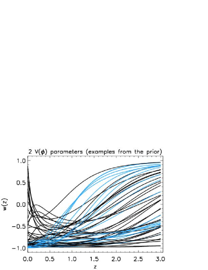
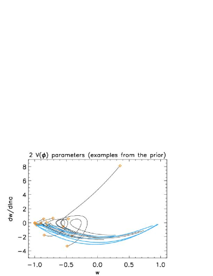
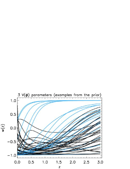
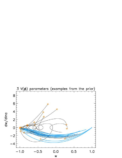
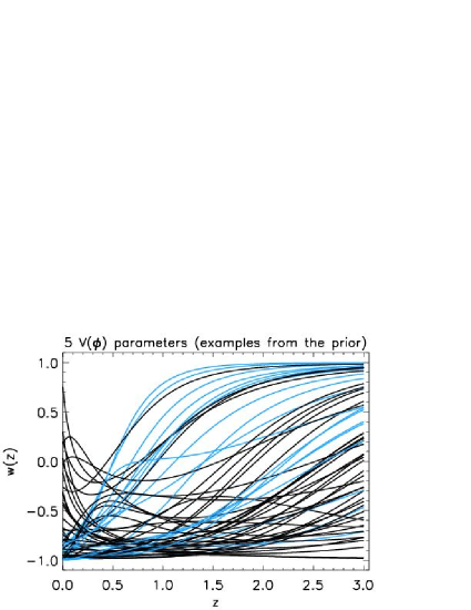
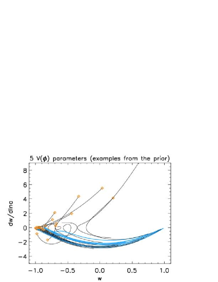
Figure 1: Left panels: representative histories $w(z)$ for a number of randomly chosen sets of initial conditions, shown for illustration without applying cosmological data constraints. Models which are freezing (see Sec. VII.2) are color-coded in blue, while the models color-coded in black are neither thawing nor freezing. We find that thawing models are very rare. Right panels: the corresponding phase plots in the $w-dw/d\ln a$ plane, showing the evolution of these parameters as a function of redshift. The evolution histories originate at $z_{\rm start}=3$. The orange diamonds represent $z=0$. The parameterization assumes 2-parameter (top row), 3-parameter (middle row) and 5-parameter (bottom row) descriptions of $V(\phi)$.

We use a Markov Chain Monte Carlo (MCMC) technique Christensen and Meyer (2000); Christensen et al. (2001); Knox et al. (2001); Lewis and Bridle (2002); Kosowsky et al. (2002); Verde et al. (2003) to evaluate the likelihood function of model parameters. The MCMC is used to simulate observations from the posterior distribution ${\cal P}({\bf\alpha}|x)$, of a set of parameters $\theta$ given event $x$, obtained via Bayes’ Theorem,

$${\cal P}(\mbox{\boldmath$\mbox{\boldmath$\theta$}$}|x)=\frac{{\cal P}(x|\mbox{\boldmath$\theta$}){\cal P}(\mbox{\boldmath$\theta$})}{\int{\cal P}(x|\mbox{\boldmath$\theta$}){\cal P}(\mbox{\boldmath$\theta$})d\mbox{\boldmath$\theta$}},$$ (12)

where ${\cal P}(x|\mbox{\boldmath$\theta$})$ is the likelihood of event $x$ given the model parameters $\theta$ and ${\cal P}(\mbox{\boldmath$\theta$})$ is the prior probability density. The MCMC generates random draws (i.e. simulations) from the posterior distribution that are a “fair” sample of the likelihood surface. From this sample, we can estimate all of the quantities of interest about the posterior distribution (mean, variance, confidence levels). A properly derived and implemented MCMC draws from the joint posterior density ${\cal P}(\mbox{\boldmath$\theta$}|x)$ once it has converged to the stationary distribution.

We use four chains per model and a conservative Gelman-Rubin convergence criterion Gelman and Rubin (1992) to determine when the chains have converged to the stationary distribution. For our application, $\theta$ denotes a set of cosmological parameters: the starting value of the energy density and equation of state of dark energy, $\Omega_{\rm DE}^{\rm start}$ and $w^{\rm start}$, and the starting values of the potential parameters as specified in Table 1. This set of parameters fully determines the dark energy history from $z=z_{\rm start}$ until today. In addition, we marginalize over the angular size of the acoustic horizon $\theta_{A}$ (a proxy for the Hubble constant $H_{0}$) and the fractional physical energy density in baryons, $\Omega_{b}h^{2}$ as nuisance parameters. The universe is assumed to be to be flat; thus the fractional matter density is given by $\Omega_{m}=1-\Omega_{\Lambda}$.

The full details of the cosmological data used, along with their likelihood functions, are given in Appendix A. Essentially, we use a combination of supernova data (Supernova Legacy Survey Astier et al. (2006)), baryon oscillation results from the Sloan Digital Sky Survey Eisenstein et al. (2005), cosmic microwave background constraints from the WMAP experiment Spergel et al. (2006), and the Hubble Key Project Freedman et al. (2001) measurement of the Hubble constant. Appendix B details the projected future cosmological data, where we assume the same cosmological probes but with the expected, smaller statistical errors (as well as estimates of the systematic errors).

Note that we do not know a priori the ranges of the initial conditions, since experimental measurements probe a specific temporal average of $\Omega_{\rm DE}$ and $w$. Therefore, we try to keep the initial conditions as general as possible, and fully marginalize over the maximally uninformative flat priors,

$$\Omega_{\rm DE}^{\rm start} \in [0,1]$$

$$w^{\rm start} \in [-1,1]$$

$$\epsilon^{\rm start} \in [0,\infty]$$

$$\eta^{\rm start} \in [-\infty,\infty]$$

$$\xi^{\rm start} \in [-\infty,30].$$ (13)

Note that we had to impose an upper limit on $\xi^{\rm start}$ in order to get the chains to converge: the upper limit in $\xi^{\rm start}$ is essentially unconstrained, both for current and future data, and our imposed limit assures convergence without affecting the results. We then apply the following Monte-Carlo algorithm:

1. Pick random initial values from the priors in Eq. (13), together with values of $\theta_{A}$ and $\Omega_{b}h^{2}$.

2. Integrate the Klein-Gordon equation; Eq. (2) to get $\Omega_{\rm DE}$ at the present epoch and $w(z)$. Compute the derived parameters $\Omega_{m}h^{2}$ and $H_{0}$, and also the principal components and $w_{0}$ and $w_{a}$ (see next Section).

3. Compute the likelihood of this model (using the likelihood functions defined in the Appendices).

4. Move to the new model using the Metropolis-Hastings sampler.

5. Repeat from step 2.

Figure 1 shows randomly chosen DE histories $w(z)$ assuming 2, 3 and 5-parameter descriptions of $V(\phi)$ (left panels; top, middle, and bottom rows respectively). For illustration, we show here the results of Monte Carlo draws from the prior, before applying cosmological constraints. To a first approximation, the three cases look qualitatively very similar. In particular, both show examples of freezing models — where $w(z)$ is asymptotically approaching $-1$ (blue curves), using the language of Caldwell and Linder Caldwell and Linder (2005), while we see very few thawing models — where $w(z)$ is asymptotically receding from $-1$. We also see examples of models that are neither purely freezing nor thawing (black curves); we comment on this in more detail in Sec. VII.2. The right panels of Figure 1 show the corresponding phase plots (i.e. the evolution of each of the models above on the $w-dw/d\ln a$ plane). These plots therefore show typical histories of $w(z)$ which are generated by the prior on the parameters which are going to be subsequently confronted with the data using the MCMC method.

Note that we have cases where $w(z_{\rm start})>0$. While these models may in principle not be ruled out by the low-z data (SNe, BAO), they may well not be viable if the energy density in DE is high enough at $z>z_{\rm start}$ to spoil the successful formation of structure. A strong test of such models is imposed by the CMB measurement of the distance to recombination, encapsulated by the angular size of the acoustic horizon $\theta_{A}$. To apply the CMB acoustic scale test, it is clear that we need to know $w(z)$ at $z>z_{\rm start}$; however this is difficult as it does not seem reasonable to extrapolate our local expansion of $V(\phi)$ to the early universe and integrate the equation for $\phi$ backward to $z\approx 1000$. Instead, we choose a simpler extrapolation in the equation of state, and assume that the equation of state is constant beyond our starting redshift, $w(z>z_{\rm start})=w(z_{\rm start})$. While somewhat ad hoc, this choice seems reasonable, as the only way that most models with $w(z>z_{\rm start})>0$ could survive the data cut is if their potential had a feature, so that $w(z)$ at high $z$ becomes again sufficiently negative. We implicitly ignore this small class of potentials that is unconstrained by the data. Further, we have repeated our analysis without the $\theta_{A}$ constraint (that is, without the constraint from distance to the last scattering surface) and found small differences at $z=z_{\rm start}$ — dark energy models with $w(z_{\rm start})>0$ are allowed without the $\theta_{A}$ essentially because the early history of dark energy is completely unconstrained in that case. However, the low-redshift constraints are nearly unchanged with or without $\theta_{A}$ imposed. Models that would be ruled out with the $\theta_{A}$ (that is, those with the “incorrect” distance to the last scattering surface) are often ruled out by the SNe+BAO+CMB+$H_{0}$ combination alone because they do not revert to being close to $\Lambda$CDM at low redshifts where the constraining power of the data is the greatest. We conclude that our ansatz $w(z>z_{\rm start})=w(z_{\rm start})$ has no discernible effects on the final low-redshift constraints.

The following sections detail the dark energy observables on which we obtain constraints.

V Derived parameters: definitions

In what follows we adopt the 2-parameter description of $V(\phi)$ (see Eq. (10)) as our fiducial case, and also consider the 3-parameter description as a test of the sensitivity of our results to the truncation of $V(\phi)$. Therefore, we have a total of at least four parameters that describe the background cosmology: at least two describing the potential ($\epsilon^{\rm start}$ and $\eta^{\rm start}$), and then $\Omega_{\rm DE}^{\rm start}$ and $w^{\rm start}$. Note that we will be mainly interested in constraints on the present-day values of the first four parameters, which we denote with the superscript “0”. Finally, we will not be very interested in the constraints on the remaining parameters, $\theta_{A}$, $H_{0}$, $\Omega_{m}h^{2}$ and $\Omega_{b}h^{2}$, because we found that, as expected, the constraints on these parameters largely reproduce the prior given to them by the observational measurements (the details of which are in the Appendices).

In addition to presenting constraints on our fiducial parameters and looking at dark energy histories via $w(z)$, we would like to report errors on the commonly used 2-parameter description of the equation of state $(w_{0},w_{a})$ where Chevallier and Polarski (2001); Linder (2003)

$$w(z)=w_{0}+w_{a}{z\over 1+z}.$$ (14)

However, as seen in Figure 1, the scalar field models evidently do not follow the relation (14) over the redshift range considered, though they (presumably) do over the range of redshifts strongly probed by the data. Therefore, we need an algorithm to assign the best-fitting $w_{0}$ and $w_{a}$ to a given dark energy history. We do that in two steps: we first determine the best-fitting principal components computed from an idealized Fisher matrix analysis, then convert the first two of them into the familiar equation of state parameters. We now describe this procedure in detail.

V.1 Principal components

A convenient way to describe a given dark energy model is to compute the best-measured principal components (PCs) of $w(z)$ for each dark energy model history Huterer and Starkman (2003). This is a form of data compression, where many parameters needed to describe the dark energy sector are replaced by a few that describe the quantities that are best measured by a given set of cosmological probes. The main advantage of the PCs is that they are model independent — in other words, they are independent of parameterizations of dark energy density or equation of state. The weight of the best-measured principal component is a model-independent predictor of what redshift range is best probed by a given cosmological probe — the first PC peaks at $z\sim 0.2$ for future SNe measurements Huterer and Starkman (2003); Crittenden and Pogosian (2005), $z\sim 0.5$ for weak lensing Linder and Huterer (2005); Simpson and Bridle (2006) and $z\sim 0.7$ for baryon oscillations. The shapes of principal components also depend, albeit more weakly, on the survey specifications and the fiducial cosmological model.

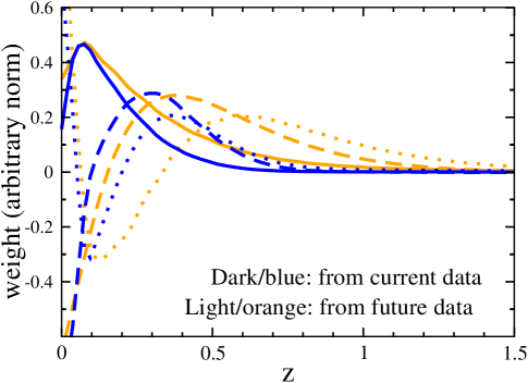
Figure 2: The first three principal components that are best measured by the current data (solid, dashed and dotted dark/blue line) and the future data (solid, dashed and dotted dark/blue line light/orange line). The components were computed starting with 40 piecewise constant values of the equation of state linearly distributed in the redshift range $0\leq z\leq 2$ and using the Fisher matrix formalism, as described in Huterer and Starkman (2003). Note that the future PCs have peak weight at somewhat higher redshifts, which directly reflects the extended redshift reach of future SNe and BAO observations.

In order to compute the principal components from a given survey, one needs to compute joint constraints on a large number of parameters that determine the function $w(z)$, then diagonalize their covariance matrix. While relatively straightforward to do in the Fisher matrix formalism and with simulated data Huterer and Starkman (2003); Hu (2002); Linder and Huterer (2005); Crittenden and Pogosian (2005); Stephan-Otto (2006); Dick et al. (2006), this task is very challenging with actual data as accurate computation of the covariance matrix of a large number ($\sim 10$-$50$) of highly correlated parameters is required, although the computational requirements are significantly less severe if one only wants a rough resolution of the principal components in redshift as done in Refs. Huterer and Cooray (2005) and Shapiro and Turner (2005).

Note that we could in principle compute the exact principal components of our scalar field model equations of state, since we have the full $w(z)$ of each model in our Markov chains; it is just a matter of outputting these quantities at a number of redshifts, computing their covariance matrix from the information in the chains, and diagonalizing it. However, the equation of state values at different redshifts in scalar field models are highly correlated since the scalar field paradigm together with the few-parameter description of the effective potential models only allows specific dark energy histories. These correlations render the principal components of the scalar field equation of state very different from the usual PCs of a general $w(z)$. While it may be of interest to work with the scalar field PCs, this is largely terra incognita, and in this work we instead concentrate on the usual PCs for a completely general $w(z)$ computed for a combination of surveys that we consider. We leave the study of scalar-field-specific PCs for future work.

Therefore, we adopt a hybrid approach here: we compute the principal components assuming a Fisher matrix as an approximation to the inverse of the true covariance matrix, and also assuming theoretically unconstrained dark energy histories. We use the actual cosmological data, current or future (from Appendices A and B), approximating the CMB information by the distance to the last scattering surface which has been marginalized over the sound horizon parameters; this analysis closely parallels that in Huterer and Starkman (2003); Linder and Huterer (2005). We parameterize the equation of state in 40 piecewise constant values uniformly distribution in $0<z<z_{\rm max}$. We evaluate the original Fisher matrix, invert it, eliminate the parameters not corresponding to $w(z)$ (such as $H_{0}$ and $\Omega_{m}$), and diagonalize the resulting matrix in the equation of state parameters to obtain the principal components.

Figure 2 shows the shapes $e_{i}(z)$ of the first three principal components of the current data (solid, dashed and dotted dark/blue line) and the future data (solid, dashed and dotted light/orange line). The curves have been smoothed in redshift with a cubic spline, and are normalized arbitrarily in this plot. Note that the weights of the future PCs peak at somewhat higher redshifts, which directly reflects the extended redshift reach of the future SNe and BAO observations.

Given a dark energy history $w(z)$, the amplitude of $i$th principal component, $\alpha_{i}$, is given by Huterer and Starkman (2003)

$$\alpha_{i}=\int_{0}^{\infty}w(z)\,e_{i}(z)\,dz$$ (15)

where the principal components are normalized so that $\int_{0}^{\infty}e_{i}(z)\,dz=1$, and the error in $\alpha_{i}$ is determined by the cosmological datasets used. For each model from the Markov chains, we compute the principal component coefficients according to Eq. (15). Given that we are now using the pre-computed principal components that are obtained for a general $w(z)$, the parameters $\alpha_{i}$ will not be uncorrelated in our scalar field dark energy analysis.

V.2 The equation of state parameters

We would also like to show our constraints in terms of more familiar 2-parameter description of dark energy $w_{0}$ and $w_{a}$. Of course, our goal is not to simply fit $(w_{0},w_{a})$ to the cosmological data as often done in the literature — instead, we seek to describe each scalar field model that we generate with some effective $(w_{0},w_{a})$. Mapping the true redshift-dependent equation of state of a model into a finite number of parameters is not trivial. The most obvious way to proceed would be to fit $(w_{0},w_{a})$, together with other cosmological parameters, to each dark energy model in our chains. Unfortunately, this procedure would be too time-consuming, as we would need to perform a multi-parameter fit to each one of millions of dark energy models that we generate in our MCMC procedure. Clearly, a faster way to construct $(w_{0},w_{a})$ is needed.

Here we propose and adopt an alternative, extremely simple algorithm: we simply convert the first two principal components $(\alpha_{1},\alpha_{2})$ into $(w_{0},w_{a})$. This approach is justified because the first two PCs carry essentially all the necessary information about the effects of dark energy dynamics on the expansion of the universe over the observable scales. From Eqs. (14) and (15) it follows that we can define

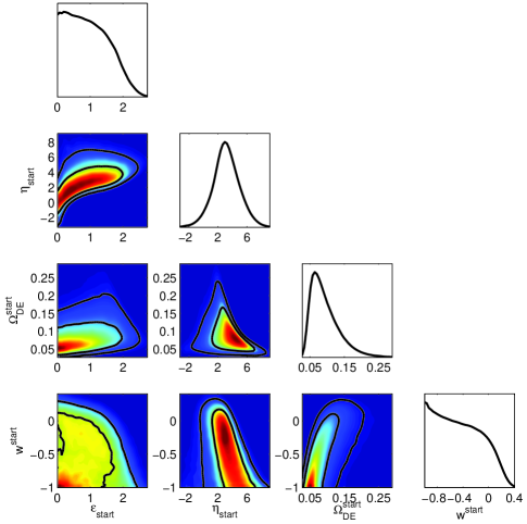
Figure 3: Solid lines show the marginalized 2D-joint 68% and 95% probability contours (off-diagonal panels) and 1D marginalized probability distribution (diagonal panels) for the two potential parameters $\epsilon$ and $\eta$, as well as $\Omega_{\rm DE}$, and $w$. The color coding in the off-diagonal panels shows the marginalized probability density in these 2D parameter spaces, ranging from red for the highest density to blue for the lowest. The left and right sets of panels show constraints at $z=0$ and $z_{\rm start}=3$ respectively, using the current cosmological data as described in Appendix A. We do not show the parameters $H_{0}$, $\Omega_{m}h^{2}$ and $\Omega_{b}h^{2}$ which largely reproduce the applied measurement priors. Note that the constraints at $z_{\rm start}=3$ are considerably weaker than at $z=0$, since the constraining power of the data is concentrated at lower redshift.

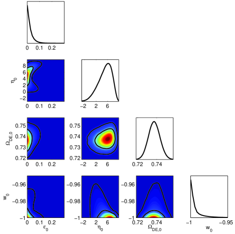
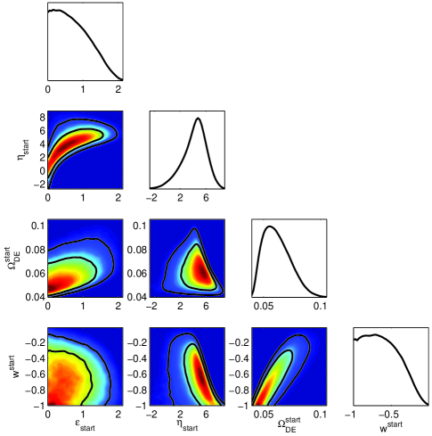
Figure 4: Same as Fig. 3, but parameter constraints are for future data as described in Appendix B, defined at $z=0$ (left) and $z_{\rm start}=3$ (right). It is interesting to note that constraints on the potential parameters $\epsilon$ and $\eta$ improve to a significantly lesser degree than those on $\Omega_{\rm DE}$ and $w$ when compared with the constraints from the current data.

$$w_{0} \equiv {\alpha_{2}\beta_{1}-\alpha_{1}\beta_{2}\over\beta_{1}-\beta_{2}}$$ (16)

$$w_{a} \equiv {\alpha_{1}-\alpha_{2}\over\beta_{1}-\beta_{2}}$$ (17)

where

$$\beta_{i}\equiv\int e_{i}(z)\,{z\over 1+z}\,dz.$$ (18)

Equations (16) and (17) are now our definitions of the parameters $w_{0}$ and $w_{a}$, given a dark energy history $w(z)$ which determines the $\alpha_{i}$. We have explicitly checked on individual examples that the two-parameter equation of state closely follows the true $w(z)$ over the redshift range most effectively probed by the data. Note too that the constraint $w_{0}\geq-1$, which follows from $w(z)\geq-1$, is not strictly obeyed by $w_{0}$ obtained in this way since $w_{0}$ and $w_{a}$ are now essentially a fit to the dark energy equation of state history. We will return to the efficacy of this approximation later in Sec. VI.4.

V.3 Equation of state pivot

The pivot value of the equation of state parameter is the value of $w(z)$ at the specific redshift where the equation of state is best constrained and has a “waist” Huterer and Turner (2001). In other words, we require that $w_{\rm pivot}=w_{0}+Aw_{a}$ and $w_{a}$ be uncorrelated, where $A$ is a coefficient to be determined. In practice, having obtained the $(w_{0},w_{a})$ corresponding to a model for each step in the Markov chains, we can compute the covariance matrix of these two parameters and diagonalize it to extract $(w_{\rm pivot},w_{a})$. It is easy to show that $A=-{\rm Cov(w_{0},w_{a})}/{\rm Cov(w_{a},w_{a})}$ and

$$w_{\rm pivot}=w_{0}-{{\rm Cov(w_{0},w_{a})}\over{\rm Cov(w_{a},w_{a})}}\,w_{a}$$ (19)

where ${\rm Cov}(x,y)$ stands for elements of the covariance matrix element. Although we make no specific use of the pivot redshift, for completeness, it is given by

$$z_{\rm pivot}=-{{\rm Cov(w_{0},w_{a})}\over{\rm Cov(w_{0},w_{a})}+{\rm Cov(w_{a},w_{a})}}.$$ (20)

Now we will present our constraints on these dark energy observables.

VI Basic results

VI.1 Fundamental parameters

In Fig. 3 we show the constraints from the current data on $\epsilon$, $\eta$, $\Omega_{\rm DE}$, and $w$ at redshift zero (left panel; superscripts “0”) and redshift $z_{\rm start}=3$ (right panel; superscripts “3”). In Fig. 4 we show the equivalent constraints for future data, assuming a $\Lambda$CDM fiducial model.

The $z=3$ constraints (right panel of Fig. 3) are not particularly tight, as the only direct probe of this redshift comes from the CMB. Nevertheless, we see that the equation of state is limited to be $w^{\rm start}\lesssim 0$; this constraint is directly due to the CMB location of the first peak $\theta_{A}$, as models with $w(z)>0$ at high redshift are increasingly dark energy dominated and produce an incorrect distance to the last scattering surface. Note that the best-fit $\Lambda$CDM cosmology has $\Omega_{\rm DE}^{\rm start}\approx 0.05$.

In contrast, constraints at $z=0$ (left panel of Fig. 3) are excellent. In particular the equation of state $w^{0}$ and the first slow-roll parameter $\epsilon^{0}$ are determined with great accuracy. Our choice to show constraints at $z=0$ is somewhat arbitrary, as we would expect similarly good constraints at $z\lesssim 0.5$ in general. Rather than these quantities at particular time slices, it is of more interest to show the reconstructed histories of dark energy, as well as quantities that reflect the time-averaged behavior of dark energy (e.g. $w_{0}$, $w_{a}$, principal components) as we do below. Nevertheless, we pause to comment that these constraints are complementary to the usual approach where the dark energy sector is parameterized via a single, constant equation of state parameter $w$. While neither one of our fundamental parameters in Fig. 3 is constant in time, the constraints on them are tight because of the combination of the theoretical prior and cosmological data. Constraints from these two different approaches, model-independent $w={\rm const}$ and scalar field time-dependent $w(z)$, do not necessarily need to be in agreement — nevertheless, we do expect many salient features to be the same, such as the preference for $\Omega_{\rm DE}^{0}\approx 0.75$ and $w^{0}\approx-1$, and this is reflected in the left panel of Fig. 3.

One interesting point to note is that the expected future constraints on the potential parameters $\epsilon$ and $\eta$ improve to a significantly lesser degree than those on $\Omega_{\rm DE}$ and $w$ when compared with the constraints from the current data. This suggests that our knowledge of the local shape of the effective potential will not improve very much in the future compared to that of the velocity and the potential energy of the field.

In our formalism we can directly compute the field excursion from $z=3$ to $z=0$ for each model in our chains by integrating Eq. (2), and hence obtain constraints on it: we find $\Delta\phi/m_{\rm pl}=0.09\pm 0.03$. Thus the field evolution in the range probed best by the data is small. Therefore it is not surprising to find that the constraints on the shape of the potential are not strong, since such a narrow range of the potential is probed. In addition, unlike in the case of inflation, there is no theoretical slow-roll prior to help constrain the shape of the potential over a larger $\phi$ range than that probed by observations.

VI.2 Principal components

Figure 5 shows the 2D-joint 68% and 95% CL constraints in the $(\alpha_{1},\alpha_{2})$ (left panel) and $(\alpha_{2},\alpha_{3})$ (right panel) planes. Constraints using the current data, described in Appendix A, are shown in blue/dark regions, while constraints from the future data, described in Appendix B, are in orange/light regions. As mentioned earlier, the future data are centered on the $\Lambda$CDM model ($\alpha_{i}=-1$ for all $i$) by fiat. We overlay the actual constraints with $\sim 1000$ models randomly selected from our prior without being subject to the data constraints. Note that the future constraints are much better than the current ones (this is further discussed in Sec. VII.1). While the density of the models itself depends on the prior, it is clear that both the current and the future data exclude a significant fraction of them. Finally, the marginalized constraints for the individual principal component parameters are shown in Table 2.

The constraints on the principal components exhibit features that are interesting to comment on. Principal components of general dark energy models are by definition uncorrelated, and this is clearly not the case from Fig. 5; the reason is, as explained in Sec. V.1, that we have used the general PCs and constrained them assuming scalar field models. The principal components are therefore correlated, but this does not change any of the scientific results in the paper.

Moreover, one can note four well-defined edges in the left panel of Fig. 5 for either dataset. The condition $\alpha_{1}\geq-1$ is always strictly obeyed since the first principal component is a non-negative weight over the equation of state and $w(z)\geq-1$ for scalar fields; see Fig. 2. For the same reason the condition $\alpha_{2}\geq-1$ is obeyed, though not strictly — the second PC has a both positive and negative weight and, for a small fraction of our $w(z)$ models, this leads to $\alpha_{2}<-1$ (a few of the dotted examples in the left panel of Fig. 5, around the value $\alpha_{1}\approx 0.7$, exhibit this behavior). The long diagonal edge seen in this panel is also due to the requirement $w(z)\geq-1$ and its precise slope and intercept are determined by the shapes of the first two principal components. Finally, the fuzzy edge with roughly $\alpha_{1}\lesssim-0.85$ (for the current data) is due to the cosmological data that effectively restrict the weighted average of the equation of state to be less than this value. This last limit is more stringent for the future data, and dotted models from the prior, which have not been subjected to the data, are obviously not restricted in this direction.

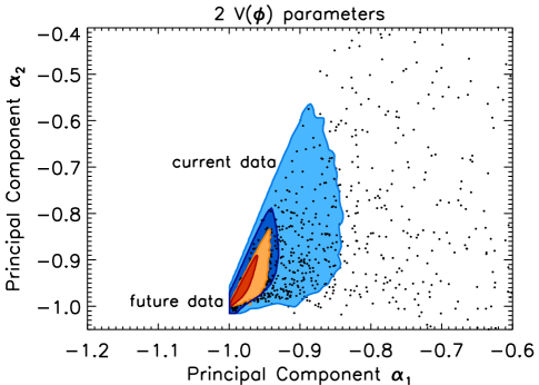
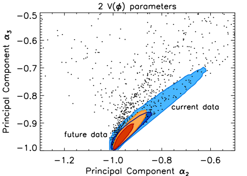
Figure 5: Left panel: 68% and 95% CL constraints from current data (larger/blue contours) and future data (smaller/orange contours) on the principal components $\alpha_{1}$ and $\alpha_{2}$. Right panel: same constraints, but on the principal components $\alpha_{2}$ and $\alpha_{3}$. The future data have been centered on the $\Lambda$CDM model ($\alpha_{i}=-1$ for all $i$), while the current data reflect the actual constraints. The points show $\sim 1000$ DE models simulated randomly from the priors, that passed our basic requirements set forth at the beginning of Sec. III but have not been subjected to the data. Note that the points lying within the region allowed by the future data constraint have been overplotted by the constraint for clarity — models from the prior go all the way down to the $\Lambda$CDM solution.

VI.3 Parameters $w_{0}$, $w_{a}$ and $w_{\rm pivot}$

Constraints in the $w_{0}$-$w_{a}$ plane are shown in the left panel of Fig. 6. As in Fig. 5, we have shown the current and future constraints (the latter assuming $\Lambda$CDM ) as well as $\sim 1000$ individual models from the prior. Moreover, there are two sharp edges that all models obey due to the requirement $w(z)\geq-1$; this is similar as with the principal components shown in Fig. 5. Likewise, the third, long side of the triangle contours are due to the cosmological data which, to a first approximation, impose an upper limit to an average of the equation of state. For the current data, this constraint is roughly $6w_{0}+w_{a}\lesssim-5$.

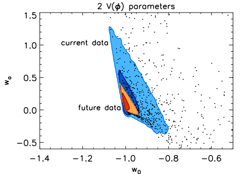
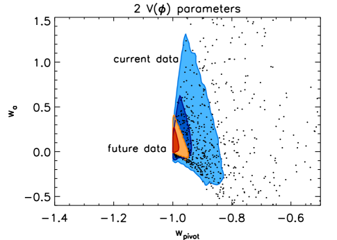
Figure 6: Left panel: 68% and 95% CL constraints from current data (larger/blue contours) and future data (smaller/orange contours) on the equation of state parameters $w_{0}$ and $w_{a}$. Right panel: same, but the parameters are now $w_{\rm pivot}$ and $w_{a}$, where the pivot $w_{\rm pivot}$ is the value of $w(z)$ at the specific redshift where $w_{0}$ and $w_{a}$ are decorrelated. As in the previous two figures, the future data have been centered on the $\Lambda$CDM model (coordinates $(-1,0)$ in both panels); the current data reflect the actual constraints, and the points show $\sim 1000$ DE models simulated randomly from the priors.

Following the simple procedure outlined in Sec. V.3, we can obtain constraints on the pivot value of the equation of state. Constraints in the $(w_{\rm pivot},w_{a})$ plane are shown in the right panel of Fig. 6. These constraints are similar to those on $(w_{0},w_{a})$ except that $w_{\rm pivot}$ and $w_{a}$ are uncorrelated by the definition of $w_{\rm pivot}$. As with the principal component $\alpha_{1}$, the relatively sharp edge at $w_{\rm pivot}=-1$ is due to the fact that $w(z)\geq-1$ for scalar field models. Future constraints are about an order of magnitude better than the current ones, as noted above.

Finally, Table 2 shows the constraints on $w_{0}$, $w_{a}$, and $w_{\rm pivot}$. Note that $w_{0}$ is a two-tailed distribution while $w_{\rm pivot}$ is a significantly skewed one-tail distribution with a hard prior $w_{\rm pivot}\geq-1$, where the probability density abruptly falls at the boundary. This is because while $w_{0}$ is allowed to go below $-1$ due to our method for assigning ($w_{0}$, $w_{a}$) for a given model $w(z)$, decorrelating these parameters recovers the prior on the original evolution histories, $w(z)\geq-1$. Further, contrary to the expectation from the usual Fisher matrix analyses, the strong non-Gaussianity of the probability distribution function means that, while the $w_{\rm pivot}$ and $w_{a}$ are decorrelated, it is not true any more that we have the best constraint on the equation of state at $z_{\rm pivot}$. However, it is still useful to go to the uncorrelated parameter basis $(w_{\rm pivot},w_{a})$ even without this latter benefit, as $w_{\rm pivot}$ is a better approximation than $w_{0}$ to the real $w(z)$ over the range probed by the data, in particular recovering the theoretical prior $w_{\rm pivot}\geq-1$.

VI.4 Equation of state reconstruction

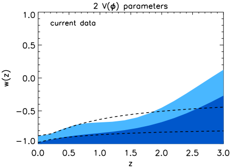
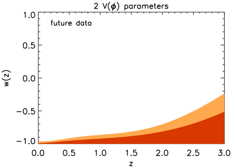
Figure 7: Shaded regions show the 68% and 95% CL constraints on the equation of state $w(z)$ from the current data (left panel) and future data (right panel). The future data assume that the fiducial cosmology is precisely $\Lambda$CDM $w(z)=-1$. In the left panel, the dashed lines show the 68% and 95% reconstruction limits using the $(w_{0},w_{a})$ parametrization. Note that the approximate $(w_{0},w_{a})$ reconstruction is in excellent agreement with the actual constraints at $z\lesssim 0.7$.

Finally, in Fig. 7 we show the 68% and 95% CL regions on the reconstructed equation of state $w(z)$. The reconstruction is straightforward, as the values of $w(z)$ at a number of redshifts are written out for each of our models as derived parameters in the MCMC. The left panel shows the constraints from the current data, while the right panel shows reconstruction from the future data. In the left panel, the dashed lines show the 68% and 95% reconstruction limits using the $(w_{0},w_{a})$ parametrization.

The constraints are very good even for the current data set. They impose a sharp upper limit on the equation of state at low redshift, and progressively get weaker at higher z. Moreover, $w(z)\lesssim 0$ is required at any redshift since otherwise, dark energy would be increasing in importance relative to matter at early times and would spoil the distance to the last scattering surface (as well as structure formation). Finally, note that the constraints using the $(w_{0},w_{a})$ parametrization are in excellent agreement with the true constraints out to $z\approx 0.7$ — therefore, our definition of $w_{0}$ and $w_{a}$, Eqs. (16) and (17), does an excellent job in reconstructing the dark energy history out to this redshift. In fact, we have checked that the rms difference between the true and $(w_{0},w_{a})$-reconstructed distance out to $z=3$ is only about 0.8% (for models from the posterior distribution for the current data), though it degrades to 3% by $z=1089$. As discussed in Sec. VII.4, the fitting accuracy to $z=3$ is significantly better (by about a factor of 4) than the accuracy to which the $z=3$ distance is determined from the current data, and therefore there is no bias in using the $(w_{0},w_{a})$ fit in this redshift range; however it is dangerous to extrapolate the fit out to higher redshift.

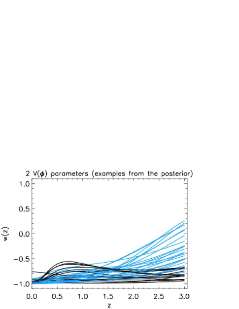
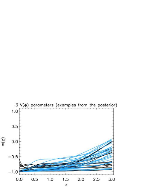
Figure 8: Follows the format of Fig. 1, except these figures show the evolution histories of a number of models which were accepted steps in the MCMC. Therefore, whereas Fig. 1 shows examples of models generated by the prior, this figure shows examples of models in the posterior.

Table 2: 68% C.L. constraints on the first three principal components, and on parameters $w_{0}$, $w_{a}$, and $w_{\rm pivot}$. The second column shows the constraints from the current data, while the third column shows errors from the future data, assuming the underlying $\Lambda$CDM cosmology (for which all parameters are $-1$ except $w_{a}$ which is zero). All rows report the usual two-sided error bars, except $w_{\rm pivot}$ where we report one-sided error bars because of the mathematical constraint $w_{\rm pivot}\geq-1$ where the probability density abruptly falls at the boundary. Recall that the constraints are significantly better than in the general non-parametric case because of the implicit theoretical prior of using scalar fields.

Parameter	Current data	Future data
$\alpha_{1}$	$-0.949^{+0.042}_{-0.050}$	fiducial${}^{+0.015}_{-0.014}$
$\alpha_{2}$	$-0.899^{+0.084}_{-0.081}$	fiducial${}^{+0.034}_{-0.033}$
$\alpha_{3}$	$-0.901^{+0.066}_{-0.065}$	fiducial${}^{+0.035}_{-0.031}$
$w_{0}$	$-0.978^{+0.032}_{-0.031}$	fiducial${}^{+0.011}_{-0.012}$
$w_{a}$	$0.197^{+0.229}_{-0.199}$	fiducial${}^{+0.089}_{-0.081}$
$w_{\rm pivot}$	$<-0.957$	$<-0.987$

Note that this Monte Carlo reconstruction is very different in spirit from the direct non-parametric reconstruction of the equation of state from distance measurements Huterer and Turner (1999); Nakamura and Chiba (1999); Saini et al. (2000); Gerke and Efstathiou (2002); Daly and Djorgovski (2004); Simon et al. (2005); Sahni and Starobinsky (2006) — the former is done via models, scalar field in this case, while the latter is completely independent of any models (although the non-parametric reconstruction still requires parametric fits to smooth the noisy distance-redshift curve observed by, say SNe Ia). Heuristically, the Monte Carlo reconstruction follows the dark energy histories generated by the assumed models, and the models correlate the equation of state values at different redshifts. This is the reason that we obtain significantly better and more reliable constraints than in the general non-parametric case. Conversely, the reconstruction presented here is clearly model-dependent, and necessarily less general than in the non-parametric case. Fig. 8 shows explicit examples of $w(z)$ histories taken from the posterior.

VI.5 Three-parameter $V(\phi)$ constraints

There is no reason to limit the effective potential to be of second order: our parametrization naturally allows potentials of arbitrary order, and we are only limited by how many parameters can be constrained with current or future data. We illustrate the constraints obtained with the polynomial of 3rd order in Fig. 10. The top left panel shows the constraints on $\epsilon^{0}$, $\eta^{0}$, $\Omega_{\rm DE}^{0}$, $w^{0}$ and $\xi^{0}$ (i.e., at $z=0$), while the top right panel shows the same constraints at $z_{\rm start}=3$. The middle row shows the constraints in the $(w_{0},w_{a})$ plane (left panel) and the $(w_{\rm pivot},w_{a})$ plane (right panel), while the bottom row show the reconstructed $w(z)$ for the current data (left panel) and future data (right panel).

The three-parameter $V(\phi)$ constraints on the five fundamental parameters are somewhat weaker than those for the two-parameter case (shown in Fig. 3). In particular, the three-parameter constraints seem to get progressively worse as we go from $\epsilon^{0}$ to $\eta^{0}$ to $\xi^{0}$. Nevertheless, the limits are still interesting, especially those on $\Omega_{\rm DE}^{0}$ and $w^{0}$. However, constraints on the parameters $w_{0}$, $w_{a}$, $w_{\rm pivot}$ and the principal components $a_{i}$ are essentially unchanged from the two-parameter case. This means that, despite the more complicated potential that is now harder to constrain, the range of dark energy histories constrained by the data is largely unchanged. This could also be seen by comparing the range of models present in the posterior distribution; see the left three panels in Fig. 1. Thus, we conclude that our constraints are only weakly sensitive to the truncation order of the polynomial series.

VI.6 (Lack of) sensitivity to initial conditions

In section III.1 we have briefly mentioned that the low redshift constraints are largely independent of the starting redshift of integration $z_{\rm start}$. We further illustrate this statement in Fig. 9 where the shaded regions show the reconstruction of the equation of state $w(z)$ for the current data as in the left panel of Fig. 7. However now the dashed lines show the reconstruction assuming the starting redshift $z_{\rm start}=5$ rather than $z_{\rm start}=3$ (the epochs $3\leq z\leq 5$ are not shown for clarity). Clearly, the constraints at $z\lesssim 0.7$ are essentially insensitive to the starting redshift.

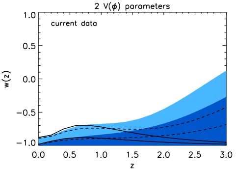
Figure 9: Shaded regions show the 68% and 95% CL constraints on the equation of state $w(z)$ from the current data, and are identical to those in the left panel of Fig. 7. Dashed lines show the reconstruction assuming the starting redshift $z_{\rm start}=5$ rather than $z_{\rm start}=3$ (the epochs $3\leq z\leq 5$ are not shown for clarity). Solid lines show the reconstruction also with $z_{\rm start}=5$, but now forcing the scalar field to start at rest (so that $w^{\rm start}=-1$). Clearly, the constraints at $z\lesssim 0.7$ are insensitive to changing the initial conditions.

Solid lines in Fig. 9 show the reconstruction of $w(z)$ also with $z_{\rm start}=5$, but now forcing the scalar field to start at rest (so that $w^{\rm start}=-1$). Clearly, the field rolls slowly in the beginning as it gains speed, and the equation of state is close to $-1$. Nevertheless, we find again that memory of this transient behavior is lost at low redshift ($z\lesssim 0.7$) where the constraints are unchanged relative to the fiducial case with unconstrained $w^{\rm start}$.

These two exercises suggest that the low redshift constraints are sensitive only to the details of the potential and not initial conditions. However, we have decided to leave a full study of this issue, including imposing physically motivated constraints on the initial conditions that take into account the field evolution at $z>z_{\rm start}$, for future work. Here we have adopted a completely empirical approach and allowed maximally general initial conditions of the scalar field.

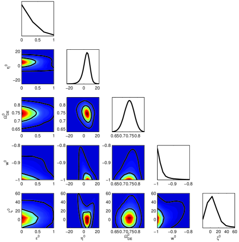
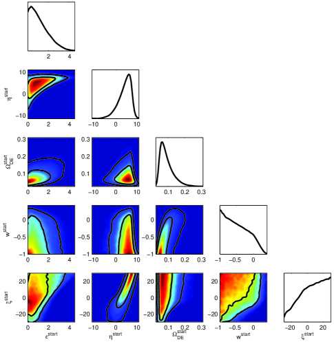
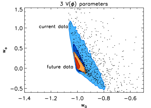
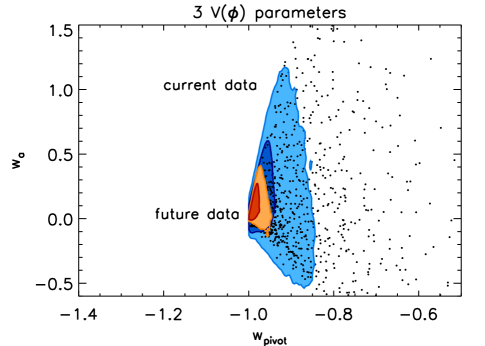
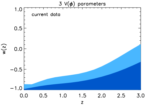
Figure 10: Constraints obtained assuming $V(\phi)$ is a polynomial of 3rd order. The top left panel shows the constraints on $\epsilon^{0}$, $\eta^{0}$, $\Omega_{\rm DE}^{0}$, $w^{0}$ and $\xi^{0}$ (i.e., at $z=0$), while the top right panel shows the same parameters evaluated at $z_{\rm start}=3$. The middle row shows the constraints in the $(w_{0},w_{a})$ plane (left panel) and the $(w_{\rm pivot},w_{a})$ plane (right panel), while the bottom row show the reconstructed $w(z)$ for the current data (left panel) and future data (right panel).

VII Cosmological Implications

We now present some implications of our constraints regarding the figures of merit, the classification of the dynamics of our models, and the preference of $\Lambda$CDM over the more complicated scalar field models. To begin with, it is clear from all results presented so far that the $\Lambda$CDM model is a very good fit to the current data. This result is in full accord with previous analyses Spergel et al. (2003, 2006); Tegmark et al. (2004); Seljak et al. (2005); Tegmark et al. (2006).

VII.1 Current vs. future data

One of the questions we set out to answer with our approach was whether it is worth pursuing future experiments, given that the current constraint are increasingly converging on the $\Lambda$CDM model. A view of Fig. 5 shows that the answer is clearly affirmative. For example, the inverse area of the 2-dimensional 68% CL contour in the $w_{0}$-$w_{a}$ plane, sometimes taken as the figure of merit for the power of cosmological constraints Huterer and Turner (2001); Albrecht et al. (2006), is about 8 times better for the future constraints than the current ones; it is 12 times better if we compare the 95% CL contour areas. For the first two principal components, the FoM is a similar factor of $\sim 10$ better for the future dataset. Clearly, if dark energy is observationally distinguishable from the $\Lambda$CDM model, upcoming surveys will have a significantly greater power to reveal this. Therefore, we eagerly expect the next generation of experiments, led by Planck, Joint Dark Energy Mission (JDEM) and Large Survey Telescope (LST).

VII.2 Thaw or freeze?

There has recently been a surge of interest in classification of dark energy models. In particular, it has been emphasized that well known dark energy models — scalar field models with potentials that are power laws or exponential functions of the field — naturally fall in classes of “thawing” or “freezing” Caldwell and Linder (2005); Linder (2006); Scherrer (2006); Chiba (2006) depending on whether they are asymptotically receding from or approaching the state of zero kinetic energy where the equation of state is $-1$. Note that freezing dark energy models have been studied at least as far back as Ratra and Peebles (1988), while thawing models date back at least to Frieman et al. (1995).

With the benefit of our framework we can quantitatively answer questions about the division of models. Our parameterization is more general than that in most previous studies as we consider all quadratic/cubic polynomials for $V(\phi)$ with maximally uninformative priors for the initial speed and energy density of the field. On the other hand, we concentrate mainly on the low redshift universe and do not attempt to model the effective potential during the “dark ages” of the universe and earlier. Therefore it is interesting to compare our findings with those from previous studies.

We define a given model as “thawing” if $dw/d\ln a>0$ uniformly, and “freezing” if $dw/d\ln a<0$ uniformly, and as neither thawing nor freezing if $dw/d\ln a$ changes sign, in the interval $z_{\rm start}=3$ to $z=0$. From our prior alone, with no data cut applied (as in left panels Fig. 1) we find that about 40% models are freezing, 0.4% are thawing, and about 60% are neither. If we consider the models in our chains, i.e. in the posterior distribution (as in Fig. 8), we find that about 74% are freezing, a negligible fraction (0.05%) are thawing, and 26% fall into neither category. Hence the thawing fraction, small to begin with, is nearly completely eliminated once the data have been applied.

One might consider that, since thawing models have $w^{\rm start}\simeq-1$ and $\Omega_{\rm DE}^{\rm start}\ll 1$ and we have uniform priors in those quantities, that the prior is biased against generating these models. However, it is not necessarily true that the posterior will therefore be biased against them. If the data clearly favored thawing models over freezing models, the MCMC would “learn” to concentrate very close to the initial conditions that favor these models. Instead we see that the fraction of freezing models in the posterior increases over that of the prior, and the already-small fraction of thawing models becomes yet smaller after the application of cosmological data, which favor models that have $w(z)\simeq-1$ at low redshifts.

This situation is analogous to the case of Monte Carlo reconstruction applied to inflation. In that prior, about 92% of models are driven to the $r=0$ late-time “attractor” solution (using a uniform prior in $\epsilon$) Kinney (2002). However, in the posterior, the models with tensor/scalar ratio $r$ up to the upper limit allowed by the data, which is significantly larger than zero, are explored very well Peiris and Easther (2006a); Peiris and Easther (2006b). In fact, a class of models which has $r\simeq 0$ and a very blue spectral index, which forms a fraction of about 90% of models generated by the prior, is completely ruled out by the data. In this sense, as long as the data have constraining power, the Metropolis-Hastings sampler does not necessarily reproduce biases due to the measure on the prior which are seen in a naive Monte-Carlo process.

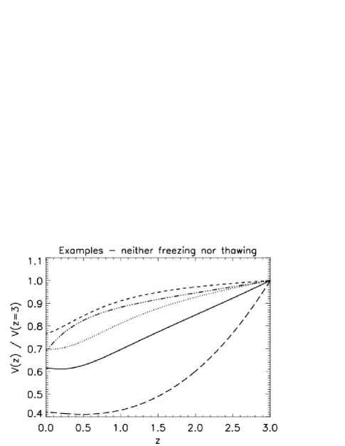
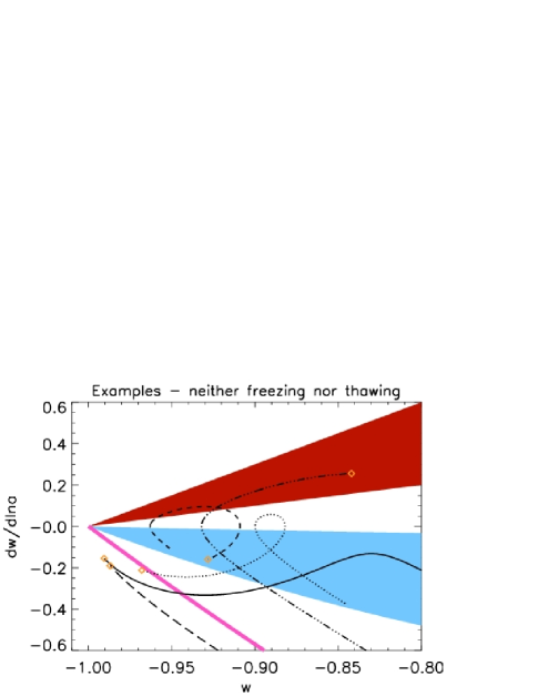
Figure 11: Several dark energy histories from our chains that are relevant to the thawing/freezing discussion. Top panel: the potentials, $V(z)/V_{0}$. Middle panel: $w(z)$ histories of these models. Bottom panel: trajectories in the $w-dw/d\ln a$ plane, together with shaded regions that should be occupied by thawing and freezing models according to Ref. Caldwell and Linder (2005), the orange diamonds again denoting $z=0$. The bottom panel plot shows that our models often do not lie solely in either region, nor do they necessarily retain their purely thawing or freezing behavior. Reasons for the disagreement are discussed in the text. The thick (pink) line in this panel shows a more general lower bound on monotonic quintessence potentials from Scherrer (2006) which is obeyed by all our models satisfying this assumption.

Notice however that our thawing/freezing classification was initiated at the time when we set initial conditions for the scalar field dynamics, $z=z_{\rm start}$, and did not allow the field to settle past the transient and into the late-time behavior. If, instead, we require $dw/d\ln a$ to have a given sign only at $z<z_{*}$ where $z_{*}<z_{\rm start}$, then the effect of the initial conditions will not be as important. With $z_{*}=1$, and looking at the posterior distribution of models, we find that the thawing fraction of models rises to 2% - still small, but much bigger than when $z_{*}=z_{\rm start}$.

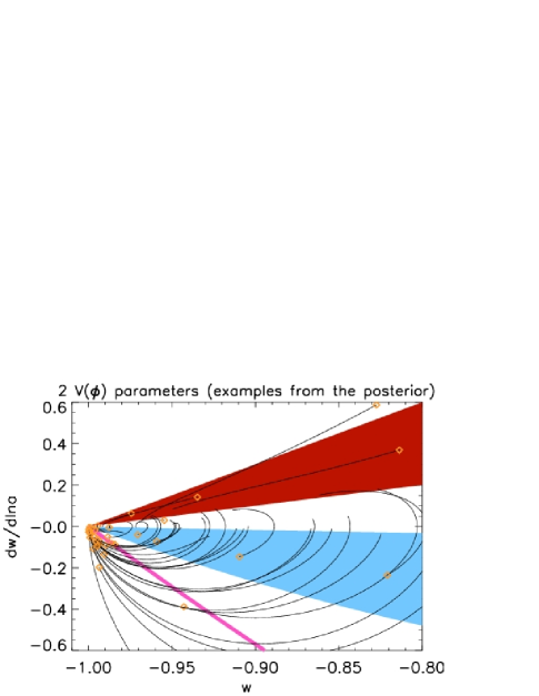
Figure 12: Typical trajectories in the $w-dw/d\ln a$ plane for a number of models in the posterior, together with shaded regions that should be occupied by thawing and freezing models according to Ref. Caldwell and Linder (2005), the orange diamonds again denoting $z=0$. The left panel shows the trajectories starting at $z_{\rm start}=3$ and the right panel shows just the region between $z=1$ and $z=0$ for the same models. The thick (pink) line in both panels shows a more general lower bound on monotonic quintessence potentials from Scherrer (2006) which is obeyed by all our models satisfying this assumption.

Several examples of dark energy models from our chains that are relevant to the thawing/freezing discussion are shown in Fig. 11. The top panel shows the potential $V(z)/V_{0}$, the middle panel shows the $w(z)$ histories, and the bottom panel shows the trajectories of these models in the $w-dw/d\ln a$ plane, together with shaded regions that should be occupied by thawing and freezing models according to Ref. Caldwell and Linder (2005). Clearly, the latter plot shows that our models often do not lie solely in either region, nor do they necessarily retain their purely thawing or freezing behavior. This remains true even if we only restrict to very late-time evolution ($z<z_{*}=1$, say). Fig. 11 also shows a thick (pink) line, a more general lower bound Scherrer (2006) which is obeyed by all monotonic quintessence potentials. This latter bound, unlike the one from Caldwell and Linder (2005), is obeyed by all our models except for those where the field samples a section of the potential that is not monotonic. Fig. 12 shows the evolution on the $w$ – $dw/d\ln a$ plane for a number of models, with the left panel showing the entire evolution from $z_{\rm start}=3$ to $z=0$, and the right panel shows only the evolution for $z<z_{*}=1$ for the same models. As the various examples in these figures illustrate, the disagreement between our models and the phenomenologically expected bounds from Caldwell and Linder (2005) is due to the interplay between the initial conditions of the scalar field, the effects of Hubble friction, and the shape of the effective potential (specifically, non-monotonicity in the second derivative) that our more general class of models possesses. For example, the short dashed example in Fig. 11 shows freezing behavior early on due to the Hubble friction; then the field velocity increases and a thawing period ensues when $H(z)$ has fallen sufficiently; but at the last, most recent stage the potential happens to flatten off and the field enters the freezing regime again. Note that the more general bound from Scherrer (2006) is again obeyed as long as the sampled potential is monotonic.

Clearly, the thawing/freezing/neither fractions depend on the particular priors – the assumed form of $V(\phi)$ and the initial conditions. Therefore it seems that, at this stage when we do not have a good theoretical understanding of dark energy, it is not useful to specialize into studying models that are thawing or freezing, because their presence or lack thereof is almost certainly not robust to fundamental assumptions. Conversely, if we ever obtain a precise measurement with a decidedly positive or negative value of $dw/d\ln a$ (or $w_{a}$, or $\alpha_{2}$), the thawing/freezing picture can help obtain a fuller theoretical understanding — a point also made by others advocating this approach Caldwell and Linder (2005); Linder (2006); Scherrer (2006); Chiba (2006).

VII.3 How many dark energy parameters?

More parameters describing the dark energy sector will lead to an improved fit to the data, but are they required by the data? This question can be answered using the Bayesian Information Criterion (BIC) statistic,

$${\rm BIC}=-2\ln\mathcal{L}_{\rm max}+D\ln N_{\rm data},$$ (21)

where $\mathcal{L}_{\rm max}$ is the maximum likelihood in a given class of models, $D$ is the number of parameters in a model, and $N_{\rm data}$ the number of data points used. A BIC difference of 2 or more indicates good evidence, and 6 and more strong evidence in favor of a model with the smaller BIC.

Here we compare the $\Lambda$CDM models which have $D=3$ parameters ($\Omega_{\rm DE}^{\rm start}$, $\theta_{A}$ and $\Omega_{b}h^{2}$) and the scalar field models with two or more additional parameters (so $D=6$ or more) describing the shape of the effective potential ($w^{\rm start}$, $\epsilon^{\rm start}$ and $\eta^{\rm start}$, plus any higher derivatives of the potential). The $\Lambda$CDM model has a slightly higher value of the best fit $\chi^{2}=-2\ln\mathcal{L}_{\rm max}$, by about unity (about 108, compared to about 107 for the two-extra-parameter scalar field models, with 119 degrees of freedom). However the penalty from the second term in Eq. (21) for the scalar field models is large, $3\ln 119\approx 14.3$, and completely overwhelms the gain from the improved likelihood fit. Therefore, the overall BIC evidence (of $+13.3$) is clear: using the current data, there is no compelling evidence whatsoever for models more complicated than $\Lambda$CDM . A more comprehensive recent analysis using Bayesian model selection, albeit using the empirical variables ($w_{0}$, $w_{a}$) to describe the evolution of the dark energy, can be found in Ref. Liddle et al. (2006).

While $\Lambda$CDM is clearly an excellent fit to the current data, there are two important caveats to keep in mind. First, it is possible that models different from ones we considered have a lower BIC than the $\sim 6$-parameter scalar field models we considered (although it is still highly unlikely they will be favored by the BIC criterion). Second, we have shown that the future data will provide a much sharper test of dark energy histories, and may possibly provide the traction to see a distinct deviation from $\Lambda$CDM . Such a development would surely provide a much needed hint about the physics of dark energy.

VII.4 Physical observables

Since we have obtained constraints using a variety of cosmological probes, it is interesting to ask which physical quantities (or alternatively, which dynamical aspects of our scalar field models) are well constrained by the data. This is a fairly complex question that we largely leave for future work — however, before concluding we make an interesting observation. We found that distances out to intermediate redshifts, $z=1$-$3$, are determined to 2-3% for the current data. For the future data, the distances will be determined to about 0.5%. Therefore, any scalar field model that does not preserve the distance to redshift $z\sim 2$ to these accuracies will be ruled out. As with all other parameter constraints we presented, we can expect that these accuracies to be somewhat degraded once we allow a completely general dark energy history, not just the class of scalar field models with a smooth potential. Nevertheless, the aforementioned numbers suggest, for example, that a cosmological probe that has ambition to significantly improve upon the current constraints should determine the mean distance to a (single) redshift $z\gtrsim 1$ to $\sim 1$% or better.

VIII Conclusions

The main motivation behind this work was to study all possible dark energy histories within a broad class of models — chosen here to be the scalar field models with an effective potential described by a polynomial series. Adapting the Monte Carlo reconstruction formalism (previously applied to inflation) to scan a wide range of dark energy models, we have generated millions of dark energy models and constrained them with the current compilation of data from the Supernova Legacy Survey Astier et al. (2006), baryon oscillation results from the Sloan Digital Sky Survey Eisenstein et al. (2005), cosmic microwave background constraints from the WMAP experiment Spergel et al. (2006), along with the measurement of the Hubble constant from the Hubble Key Project Freedman et al. (2001). We have also simulated expected future data from the same cosmological probes. Instead of attempting to study comparative merits of specific cosmological probes or optimal survey designs, we have concentrated on addressing a more general set of issues regarding the future quest for dark energy.

In particular, we have addressed how the theoretical prior — working within a specific class of scalar field models parameterized with a polynomial series in $V(\phi)$ — combines with the cosmological data to produce the constraints on cosmological parameters. We found that the theoretical prior is significant, as only specific smooth dark energy histories are generated, and that their qualitative nature does not vary significantly with the order of the polynomial $V(\phi)$; see Figs. 1 and 8. Moreover, the same theoretical prior excludes certain regions of parameter space (especially in the equation of state parameters), and makes the posterior distribution highly non-Gaussian. As a consequence, the commonly used Fisher matrix formalism applied to the equation of state parameters, which assumes Gaussianity of the likelihood, could be a terrible approximation to the exact likelihood in a specific class of dark energy models, and would significantly bias the constraints. A more general approach such as the one we have adopted, Markov Chain Monte Carlo combined with an exact integration of the dark energy evolution equations, is needed. The constraints we have obtained on the fundamental parameters are shown in Figs. 3 and 4.

We have computed the principal components of the equation of state for our data compilation. As noted in Sec. V.1, and for reasons listed there, these principal components have been pre-computed for the same survey but assuming a general DE history; therefore they are not uncorrelated. Nevertheless, we find them very useful — for example, Figure 5 shows that the current data roughly imply $\alpha_{1}\lesssim-0.85$, thereby imposing an effective upper limit to the weighted average of the equation of state. Moreover, in Sec. V.2 we propose a shortcut to compute the parameters $w_{0}$ and $w_{a}$ that approximately describe the equation of state history $w(z)$ at low redshift where the constraining power of the data is the greatest. Instead of fitting $(w_{0},w_{a})$, we obtain them directly from the first two principal components. The left panel of Fig. 7 illustrates that the approximate $(w_{0},w_{a})$ description of the models fits the dark energy histories almost perfectly at $z\lesssim 1$; we found that even distances to $z=3$ are recovered to within 2-3%. These results suggest that converting from the principal components to an arbitrary parametrization can be performed with very small biases, and essentially at no additional computational cost.

The constraints in the $(w_{0},w_{a})$ or $(w_{\rm pivot},w_{a})$ planes indicate that the constraints with future data will have the (inverse area) figure of merit improvement of about an order of magnitude over the current data. Given that our models approach the currently favored $\Lambda$CDM cosmology arbitrarily closely, this means that efforts to pursue upcoming experimental efforts, such as Planck, JDEM, LST, the planned probes of baryon acoustic oscillations, and the improved Hubble constant measurements are extremely valuable and likely to lead to significant improvement in sweeping away a large fraction of currently viable models.

We have also considered the classification of models into “thawing” and “freezing” depending on whether they are asymptotically receding from or approaching the state of zero kinetic energy where the equation of state is $-1$. We found that the thawing and freezing limits on monomial-potential scalar field models, presented in Ref. Caldwell and Linder (2005), are largely not obeyed by our models. As illustrated in Fig. 11, this is due to the interplay between the initial conditions of the scalar field, the effects of Hubble friction, and the shape of the effective potential (non-monotonicity in the second derivative) that empirically generated models possess. As we do not have a good understanding behind the physical mechanism that powers dark energy, we think that the division of models into thawing and freezing, or any similar nomenclature, is useful only in the context of future experimental constraints: if the constrained phase space ends up favoring one of these subclasses, this division can help obtain a fuller theoretical understanding

Finally note that the approach that we outlined can be trivially generalized to consider, for example, the density perturbations of dark energy. By solving the perturbation equations for each model along with the background evolution equations as currently done, we can generate trajectories using the MCMC approach. Therefore, a exhaustive “scan” through the possible perturbation scenarios can be obtained, paired with the background evolution histories, and then constrained with cosmological data. This approach would nicely complement the previous analyses that largely relied on standard phenomenological descriptions of the dark energy sector Bean and Dore (2004); Weller and Lewis (2003); Hannestad (2005); Battye and Moss (2006).

This is an excellent time to perform numerically rigorous, comprehensive analyses of dark energy models because the data is finally allowing precision tests of dark energy. Not only are the statistical errors respectable (see Table 2), but most of the experiments are now reporting careful analyses of systematic errors. As we have shown in this paper, data expected in the next $\sim 10$ years will lead to precision measurements of the parameters describing the effects of dark energy on the expansion history of the universe. One can sincerely hope, perhaps even expect, that these efforts will lead to important hints as to the nature and the origin of dark energy.

Appendix A Current Cosmological data and the likelihood function

Here we report on the current cosmological observations that we use in order to constrain the cosmological models. We use a combination of SNe Ia, baryon oscillation and Hubble constant measurements, together with WMAP constraints on the angular size of the sound horizon, and the physical matter and baryon densities.

The SNa Ia data we use are Supernova Legacy Survey data from Ref. Astier et al. (2006) with $N=115$ SNa measurements, which include the low-redshift Calan-Tololo sample. The observed apparent magnitude is given by

$$m_{i}=5\log H_{0}d_{L}(z_{i})+\mathcal{M}+\alpha(s_{i}-1)+\beta c_{i}+\epsilon_{i}\,,$$ (22)

where $i=1\ldots 115$ runs through the observed SNe. The measured values of the apparent magnitude of supernova $m_{i}$, its redshift $z_{i}$, stretch $s_{i}$, color $c_{i}$ and total error $\epsilon_{i}$ are given in the SNLS paper Astier et al. (2006). The nuisance parameter $\mathcal{M}$ is a combination of Hubble parameter and absolute magnitude of SNe Perlmutter et al. (1999). The likelihood of measuring the cosmological parameter set $\theta$ is given by

$$\mathcal{L}_{\rm SNe}({\mbox{\boldmath$\theta$}}) = \int\exp(-\chi^{2}/2)\,\mathcal{P}(\alpha)\mathcal{P}(\beta)\,d\mathcal{M}\,d\alpha\,d\beta$$ (23)

$$\chi^{2}({\mbox{\boldmath$\theta$}}) = \sum_{i=1}^{N}{(m_{i}-m({\mbox{\boldmath$\theta$}},z_{i}))^{2}\over\epsilon_{i}^{2}},$$ (24)

where $\mathcal{P}(\alpha)$ and $\mathcal{P}(\beta)$ are priors given to the stretch and color coefficients. Since $\mathcal{M}$ is given a flat prior, the $\mathcal{M}$ integral can be done analytically Nesseris and Perivolaropoulos (2005) to obtain

$$\mathcal{L}_{\rm SNe}({\mbox{\boldmath$\theta$}}) = \int\exp(-(A-B^{2}/C)/2)\,\mathcal{P}(\alpha)\mathcal{P}(\beta)\,d\alpha\,d\beta$$

$$A \equiv \sum_{i=1}^{N}{(m_{i}-m({\mbox{\boldmath$\theta$}},z_{i}))^{2}\over\epsilon_{i}^{2}}$$ (25)

$$B \equiv \sum_{i=1}^{N}{m_{i}-m({\mbox{\boldmath$\theta$}},z_{i})\over\epsilon_{i}^{2}}$$ (26)

$$C \equiv \sum_{i=1}^{N}{1\over\epsilon_{i}^{2}}$$ (27)

Finally, we follow the SNLS analysis and adopt the $\Lambda$CDM values for the stretch and color parameters, $\alpha=1.52\pm 0.14$ and $\beta=1.57\pm 0.15$, and marginalize with flat priors over the $\pm 1$-$\sigma$ values in $\alpha$ and $\beta$. After experimenting with several alternative prior widths for the stretch and color coefficients, we conclude that their details introduce unobservable changes in our results.

SNe Ia provide the best constraints at low redshifts ($z\lesssim 1.7$). However, Figure 1 shows that there exist classes of models that look roughly like the cosmological constant at those redshifts but dominate the energy density at $z\gtrsim 2$. Those models are not ruled out by the SN data, but nevertheless are clearly inconsistent with the observed universe as they prevent sufficient structure formation. In order to protect against such models, we use the information provided by baryon oscillations and CMB measurements of the angular size of the acoustic horizon and the physical matter density. More precisely, we use the quantity probed by baryon oscillations

$$D_{V}(z=0.35)\equiv\left[r(z)^{2}{cz\over H(z)}\right]^{1/3}=(1370\pm 64)\,\,{\rm Mpc}$$ (28)

where $r(z)$ is the comoving angular diameter distance to redshift $z$ and the measurement comes from the Sloan Digital Sky Survey Eisenstein et al. (2005).

To represent the CMB measurements given by the WMAP experiment Spergel et al. (2003, 2006), we do not use the full likelihood function as its evaluation would be very time consuming for the millions of models we consider. Instead, an excellent approximation is to use the single derived quantity that is sensitive to dark energy, the angular size of the sound horizon Hu et al. (2001); Frieman et al. (2003), which is equal to the ratio of the physical size of the sound horizon and the distance to recombination

$$\theta_{A}\equiv{s_{H}\over r(z=1089)}=(0.595\pm 0.002)\,\,{\rm deg},$$ (29)

where the sound horizon $s_{H}$ is given by

$$s_{H}={c\over\sqrt{3}H_{0}}\int_{0}^{a_{\rm dec}}\left[\left(1+{3\Omega_{b}\over 4\Omega_{\gamma}}a\right)\left(\Omega_{m}\,a+\Omega_{R}\right)\right]^{-1/2}\,da,$$ (30)

where $\Omega_{\gamma}$ and $\Omega_{R}$ are the energy densities in photons and radiation (photons plus neutrinos) respectively. The quantities $\Omega_{\gamma}$ and $\Omega_{R}$ are given in terms of the CMB temperature and are exceedingly accurately measured, so we hold them fixed.

Finally, since $\theta_{A}$, $\Omega_{m}h^{2}$ and $\Omega_{b}h^{2}$ are our original parameters, and we compute the equation of state history $w(z)$ for each model, the Hubble constant $H_{0}$ is necessarily a derived parameter. To compute the distance to decoupling $r(z=1089)$ we use not the exact $w(z)$, but rather the constant effective equation of state $w_{\rm eff}$, defined as

$$w_{\rm eff}\equiv{\displaystyle\int_{1/(1+1089)}^{1}\Omega_{\rm DE}(a)\,w(a)\,da\over\displaystyle\int_{1/(1+1089)}^{1}\Omega_{\rm DE}(a)\,da}.$$ (31)

The reason we use $w_{\rm eff}$ is that the original WMAP analysis Spergel et al. (2006) uses a constant equation of state to arrive at their constraints.

We adopt the the physical baryon density $\Omega_{b}h^{2}$ as a free parameter and give it the prior consistent with WMAP, $\Omega_{b}h^{2}=0.0223\pm 0.00074$. The physical matter density, $\Omega_{m}h^{2}$, is also a free parameter accurately constrained by the CMB. Since our models allow more complex behavior in the dark energy sector, we conservatively double the reported $\Lambda$CDM error in this parameter, adopting $\Omega_{m}h^{2}=0.127\pm 0.02$.

Finally we adopt the Hubble Key project measurement of the Hubble constant, $H_{0}=0.72\pm 0.08$ Freedman et al. (2001). The final likelihood is

$$\mathcal{L}({\mbox{\boldmath$\theta$}})=\mathcal{L}_{\rm SNe}({\mbox{\boldmath$\theta$}})\times\mathcal{L}_{\rm BAO}({\mbox{\boldmath$\theta$}})\times\mathcal{L}_{\rm CMB}({\mbox{\boldmath$\theta$}})\times\mathcal{L}_{\rm H_{0}}({\mbox{\boldmath$\theta$}})$$ (32)

where the SNe likelihood is specified in Eq. (24), the BAO and $H_{0}$ are Gaussian with means and standard deviations specified above, and the CMB likelihood consists of $\theta_{A}$, $\Omega_{b}h^{2}$ and $\Omega_{m}h^{2}$ constraints, all of which are Gaussian with means and standard deviations specified above.

Appendix B Future data

To simulate the future cosmological data, we consider the same cosmological probes as for the current data: type Ia supernovae, baryon acoustic oscillations, CMB measurements of the sound horizon, $\Omega_{m}h^{2}$ and $\Omega_{b}h^{2}$, and the measurements of the Hubble constant. Since we obviously do not know which cosmological model will be favored by future data, we center all observables on the $\Lambda$CDM model with $\Omega_{m}=1-\Omega_{\rm DE}(z=0)=0.25$, $w(z)=-1$ and $H_{0}=0.72$. As described below, we add best-guess systematic errors for all future measurements.

For the SNa data we assume a SNAP-type experiment with 2800 SNe distributed in redshift out to $z=1.7$ as given by the middle curve of Fig. 9 in Ref. Aldering et al. (2004), and combined with 300 local supernovae uniformly distributed in the $z=0.03-0.08$ range. We add systematic errors in quadrature with intrinsic random Gaussian errors of 0.15 mag per SNe. The systematic errors create an effective error floor of $0.02\,(1+z_{i})/2.7$ mag per bin of $\Delta z=0.1$ centered at redshift $z_{i}$.

Specifications of proposed future baryon oscillation surveys and their expected statistical and systematic errors are described in the Dark Energy Task Force report Albrecht et al. (2006) (this is partly based on other studies, such as Blake et al. (2006)). To a very good approximation, baryon oscillations provide measurements of the angular diameter distance $d_{A}(z)$ and the expansion rate $H(z)$ out to the redshift(s) where the source population of galaxies is located. We adopt the DETF findings and assume a JDEM-type survey covering the redshift range $z\in[0.5,2.0]$ of 10,000 square degrees. For simplicity we assume only three redshift bins centered at $z=0.75$, $1.25$ and $1.75$ with widths $\Delta z=0.5$ each. With these parameters, formulae in the baryon oscillation section of the DETF report indicate that the total expected error (statistical plus systematic) for a spectroscopic survey is about 1.5% for the measurements of the angular diameter distance in each bin, and 2% for measurements of the expansion rate $H(z)$. Therefore we assume a total of six BAO observables – three distances and three expansion rates – with the aforementioned errors.

Note that, in the DETF error budget, a conservative 1% systematic error is assumed in each bin for each BAO observable. Controlling the systematics to a level lower than this, as well as increasing the observed sky area, would enable a future JDEM BAO mission to achieve significantly higher sensitivities than assumed here (C. Bennett, private communication). Similarly, if the JDEM SNa systematics can be understood to better than the systematics floor we assumed, the sensitivity of that experiment could be higher.

For the future CMB experiment we assume Planck The Planck Collaboration which is scheduled for launch in 2008. Planck’s fiducial error in $\Omega_{m}h^{2}$, for a flat $\Lambda$CDM universe, is about 1%. Since we are considering models with a complicated dark energy sector, we conservatively double this uncertainty, just as in the case with current data. With the assumed cosmology, this amounts to assuming $\Omega_{m}h^{2}=0.1296\pm 0.00270$. The angular size of the acoustic horizon for the fiducial cosmology and its expected Planck error are $\theta_{A}=(0.595\pm 0.00017)$ deg. Similarly, the baryon fraction is assumed to be $\Omega_{b}h^{2}=0.023\pm 0.00015$

Finally, we conservatively assume independent future measurements of the Hubble constant will reach the 5% level (more accurate measurements are feasible in principle, but the systematics remain the primary obstacles). Therefore we take $H_{0}=0.72\pm 0.036$.

The full likelihood function is given again by Eq. (32).

References

- Perlmutter et al. (1999) S. Perlmutter et al. (Supernova Cosmology Project), Astrophys. J. 517, 565 (1999), eprint astro-ph/9812133.
- Riess et al. (1998) A. G. Riess et al. (Supernova Search Team), Astron. J. 116, 1009 (1998), eprint astro-ph/9805201.
- Knop et al. (2003) R. A. Knop et al. (Supernova Cosmology Project), Astrophys. J. 598, 102 (2003), eprint astro-ph/0309368.
- Riess et al. (2004) A. G. Riess et al. (Supernova Search Team), Astrophys. J. 607, 665 (2004), eprint astro-ph/0402512.
- Astier et al. (2006) P. Astier et al., Astron. Astrophys. 447, 31 (2006), eprint astro-ph/0510447.
- Cooray and Huterer (1999) A. R. Cooray and D. Huterer, Astrophys. J. 513, L95 (1999), eprint astro-ph/9901097.
- Linder (2003) E. V. Linder, Phys. Rev. Lett. 90, 091301 (2003), eprint astro-ph/0208512.
- Corasaniti and Copeland (2003) P. S. Corasaniti and E. J. Copeland, Phys. Rev. D67, 063521 (2003), eprint astro-ph/0205544.
- Hannestad and Mortsell (2004) S. Hannestad and E. Mortsell, JCAP 0409, 001 (2004), eprint astro-ph/0407259.
- Huterer and Turner (1999) D. Huterer and M. S. Turner, Phys. Rev. D60, 081301 (1999), eprint astro-ph/9808133.
- Nakamura and Chiba (1999) T. Nakamura and T. Chiba, Mon. Not. Roy. Astron. Soc. 306, 696 (1999), eprint astro-ph/9810447.
- Starobinsky (1998) A. A. Starobinsky, JETP Lett. 68, 757 (1998), eprint astro-ph/9810431.
- Eisenstein et al. (1999) D. J. Eisenstein, W. Hu, and M. Tegmark, Astrophys. J. 518, 2 (1999), eprint astro-ph/9807130.
- Huterer and Turner (2001) D. Huterer and M. S. Turner, Phys. Rev. D64, 123527 (2001), eprint astro-ph/0012510.
- Weller and Albrecht (2002) J. Weller and A. Albrecht, Phys. Rev. D65, 103512 (2002), eprint astro-ph/0106079.
- Weller and Albrecht (2001) J. Weller and A. Albrecht, Phys. Rev. Lett. 86, 1939 (2001), eprint astro-ph/0008314.
- Maor et al. (2002) I. Maor, R. Brustein, J. McMahon, and P. J. Steinhardt, Phys. Rev. D65, 123003 (2002), eprint astro-ph/0112526.
- Kujat et al. (2002) J. Kujat, A. M. Linn, R. J. Scherrer, and D. H. Weinberg, Astrophys. J. 572, 1 (2002), eprint astro-ph/0112221.
- Bassett et al. (2004) B. A. Bassett, P. S. Corasaniti, and M. Kunz, Astrophys. J. 617, L1 (2004), eprint astro-ph/0407364.
- Bassett (2005) B. A. Bassett, Phys. Rev. D71, 083517 (2005), eprint astro-ph/0407201.
- Knox et al. (2006) L. Knox, Y.-S. Song, and H. Zhan (2006), eprint astro-ph/0605536.
- Virey and Ealet (2006) J.-M. Virey and A. Ealet (2006), eprint astro-ph/0607589.
- Melchiorri et al. (2003) A. Melchiorri, L. Mersini-Houghton, C. J. Odman, and M. Trodden, Phys. Rev. D68, 043509 (2003), eprint astro-ph/0211522.
- Corasaniti et al. (2004) P. S. Corasaniti, M. Kunz, D. Parkinson, E. J. Copeland, and B. A. Bassett, Phys. Rev. D70, 083006 (2004), eprint astro-ph/0406608.
- Spergel et al. (2003) D. N. Spergel et al. (WMAP), Astrophys. J. Suppl. 148, 175 (2003), eprint astro-ph/0302209.
- Spergel et al. (2006) D. N. Spergel et al. (2006), eprint astro-ph/0603449.
- Tegmark et al. (2004) M. Tegmark et al. (SDSS), Phys. Rev. D69, 103501 (2004), eprint astro-ph/0310723.
- Seljak et al. (2005) U. Seljak et al. (SDSS), Phys. Rev. D71, 103515 (2005), eprint astro-ph/0407372.
- Upadhye et al. (2005) A. Upadhye, M. Ishak, and P. J. Steinhardt, Phys. Rev. D72, 063501 (2005), eprint astro-ph/0411803.
- Xia et al. (2006) J.-Q. Xia, G.-B. Zhao, B. Feng, H. Li, and X. Zhang, Phys. Rev. D73, 063521 (2006), eprint astro-ph/0511625.
- Zhao et al. (2006) G.-B. Zhao, J.-Q. Xia, B. Feng, and X. Zhang (2006), eprint astro-ph/0603621.
- Nesseris and Perivolaropoulos (2005) S. Nesseris and L. Perivolaropoulos, Phys. Rev. D72, 123519 (2005), eprint astro-ph/0511040.
- Jarvis et al. (2006) M. Jarvis, B. Jain, G. Bernstein, and D. Dolney, Astrophys. J. 644, 71 (2006), eprint astro-ph/0502243.
- Doran et al. (2006) M. Doran, G. Robbers, and C. Wetterich (2006), eprint astro-ph/0609814.
- Saini et al. (2000) T. D. Saini, S. Raychaudhury, V. Sahni, and A. A. Starobinsky, Phys. Rev. Lett. 85, 1162 (2000), eprint astro-ph/9910231.
- Huterer (2002) D. Huterer, Phys. Rev. D65, 063001 (2002), eprint astro-ph/0106399.
- Takada and Jain (2004) M. Takada and B. Jain, Mon. Not. Roy. Astron. Soc. 348, 897 (2004), eprint astro-ph/0310125.
- Seo and Eisenstein (2003) H.-J. Seo and D. J. Eisenstein, Astrophys. J. 598, 720 (2003), eprint astro-ph/0307460.
- Alam et al. (2004) U. Alam, V. Sahni, and A. A. Starobinsky, JCAP 0406, 008 (2004), eprint astro-ph/0403687.
- Jonsson et al. (2004) J. Jonsson, A. Goobar, R. Amanullah, and L. Bergstrom (2004), eprint astro-ph/0404468.
- Feng et al. (2005) B. Feng, X.-L. Wang, and X.-M. Zhang, Phys. Lett. B607, 35 (2005), eprint astro-ph/0404224.
- Jassal et al. (2005) H. K. Jassal, J. S. Bagla, and T. Padmanabhan, Mon. Not. Roy. Astron. Soc. 356, L11 (2005), eprint astro-ph/0404378.
- Wang and Tegmark (2005) Y. Wang and M. Tegmark, Phys. Rev. D71, 103513 (2005), eprint astro-ph/0501351.
- Wang and Mukherjee (2006) Y. Wang and P. Mukherjee (2006), eprint astro-ph/0604051.
- Shafieloo et al. (2006) A. Shafieloo, U. Alam, V. Sahni, and A. A. Starobinsky, Mon. Not. Roy. Astron. Soc. 366, 1081 (2006), eprint astro-ph/0505329.
- Huterer and Cooray (2005) D. Huterer and A. Cooray, Phys. Rev. D71, 023506 (2005), eprint astro-ph/0404062.
- Sahlen et al. (2005) M. Sahlen, A. R. Liddle, and D. Parkinson, Phys. Rev. D72, 083511 (2005), eprint astro-ph/0506696.
- Ratra and Peebles (1988) B. Ratra and P. J. E. Peebles, Phys. Rev. D37, 3406 (1988).
- Wetterich (1988) C. Wetterich, Nucl. Phys. B302, 668 (1988).
- Frieman et al. (1995) J. A. Frieman, C. T. Hill, A. Stebbins, and I. Waga, Phys. Rev. Lett. 75, 2077 (1995), eprint astro-ph/9505060.
- Coble et al. (1997) K. Coble, S. Dodelson, and J. A. Frieman, Phys. Rev. D55, 1851 (1997), eprint astro-ph/9608122.
- Ferreira and Joyce (1998) P. G. Ferreira and M. Joyce, Phys. Rev. D58, 023503 (1998), eprint astro-ph/9711102.
- Zlatev et al. (1999) I. Zlatev, L.-M. Wang, and P. J. Steinhardt, Phys. Rev. Lett. 82, 896 (1999), eprint astro-ph/9807002.
- Liddle and Scherrer (1998) A. R. Liddle and R. J. Scherrer, Phys. Rev. D59, 023509 (1998), eprint astro-ph/9809272.
- Liddle et al. (1994) A. R. Liddle, P. Parsons, and J. D. Barrow, Phys. Rev. D50, 7222 (1994), eprint astro-ph/9408015.
- Kinney (2002) W. H. Kinney, Phys. Rev. D66, 083508 (2002), eprint astro-ph/0206032.
- Grivell and Liddle (2000) I. J. Grivell and A. R. Liddle, Phys. Rev. D61, 081301 (2000), eprint astro-ph/9906327.
- Hoffman and Turner (2001) M. B. Hoffman and M. S. Turner, Phys. Rev. D64, 023506 (2001), eprint astro-ph/0006321.
- Easther and Kinney (2003) R. Easther and W. H. Kinney, Phys. Rev. D67, 043511 (2003), eprint astro-ph/0210345.
- Peiris et al. (2003) H. V. Peiris et al., Astrophys. J. Suppl. 148, 213 (2003), eprint astro-ph/0302225.
- Peiris and Easther (2006a) H. Peiris and R. Easther, JCAP 0607, 002 (2006a), eprint astro-ph/0603587.
- Peiris and Easther (2006b) H. Peiris and R. Easther (2006b), eprint astro-ph/0609003.
- Liddle (2003) A. R. Liddle, Phys. Rev. D68, 103504 (2003), eprint astro-ph/0307286.
- Christensen and Meyer (2000) N. Christensen and R. Meyer (2000), eprint astro-ph/0006401.
- Christensen et al. (2001) N. Christensen, R. Meyer, L. Knox, and B. Luey, Class. Quant. Grav. 18, 2677 (2001), eprint astro-ph/0103134.
- Knox et al. (2001) L. Knox, N. Christensen, and C. Skordis, Astrophys. J. 563, L95 (2001), eprint astro-ph/0109232.
- Lewis and Bridle (2002) A. Lewis and S. Bridle, Phys. Rev. D66, 103511 (2002), eprint astro-ph/0205436.
- Kosowsky et al. (2002) A. Kosowsky, M. Milosavljevic, and R. Jimenez, Phys. Rev. D66, 063007 (2002), eprint astro-ph/0206014.
- Verde et al. (2003) L. Verde et al., Astrophys. J. Suppl. 148, 195 (2003), eprint astro-ph/0302218.
- Gelman and Rubin (1992) A. Gelman and D. Rubin, Statistical Science 7, 452 (1992).
- Eisenstein et al. (2005) D. J. Eisenstein et al., Astrophys. J. 633, 560 (2005), eprint astro-ph/0501171.
- Freedman et al. (2001) W. L. Freedman et al., Astrophys. J. 553, 47 (2001), eprint astro-ph/0012376.
- Caldwell and Linder (2005) R. R. Caldwell and E. V. Linder, Phys. Rev. Lett. 95, 141301 (2005), eprint astro-ph/0505494.
- Chevallier and Polarski (2001) M. Chevallier and D. Polarski, Int. J. Mod. Phys. D10, 213 (2001), eprint gr-qc/0009008.
- Huterer and Starkman (2003) D. Huterer and G. Starkman, Phys. Rev. Lett. 90, 031301 (2003), eprint astro-ph/0207517.
- Crittenden and Pogosian (2005) R. G. Crittenden and L. Pogosian (2005), eprint astro-ph/0510293.
- Linder and Huterer (2005) E. V. Linder and D. Huterer, Phys. Rev. D72, 043509 (2005), eprint astro-ph/0505330.
- Simpson and Bridle (2006) F. Simpson and S. Bridle, Phys. Rev. D73, 083001 (2006), eprint astro-ph/0602213.
- Hu (2002) W. Hu, Phys. Rev. D66, 083515 (2002), eprint astro-ph/0208093.
- Stephan-Otto (2006) C. Stephan-Otto, Phys. Rev. D74, 023507 (2006), eprint astro-ph/0605403.
- Dick et al. (2006) J. Dick, L. Knox, and M. Chu, JCAP 0607, 001 (2006), eprint astro-ph/0603247.
- Shapiro and Turner (2005) C. Shapiro and M. S. Turner (2005), eprint astro-ph/0512586.
- Gerke and Efstathiou (2002) B. F. Gerke and G. Efstathiou, Mon. Not. Roy. Astron. Soc. 335, 33 (2002), eprint astro-ph/0201336.
- Daly and Djorgovski (2004) R. A. Daly and S. G. Djorgovski, Astrophys. J. 612, 652 (2004), eprint astro-ph/0403664.
- Simon et al. (2005) J. Simon, L. Verde, and R. Jimenez, Phys. Rev. D71, 123001 (2005), eprint astro-ph/0412269.
- Sahni and Starobinsky (2006) V. Sahni and A. Starobinsky (2006), eprint astro-ph/0610026.
- Tegmark et al. (2006) M. Tegmark et al. (2006), eprint astro-ph/0608632.
- Albrecht et al. (2006) A. Albrecht et al. (2006), eprint astro-ph/0609591.
- Linder (2006) E. V. Linder, Phys. Rev. D73, 063010 (2006), eprint astro-ph/0601052.
- Scherrer (2006) R. J. Scherrer, Phys. Rev. D73, 043502 (2006), eprint astro-ph/0509890.
- Chiba (2006) T. Chiba, Phys. Rev. D73, 063501 (2006), eprint astro-ph/0510598.
- Gonzalez-Diaz (2000) P. F. Gonzalez-Diaz, Phys. Rev. D62, 023513 (2000), eprint astro-ph/0004125.
- Liddle et al. (2006) A. R. Liddle, P. Mukherjee, D. Parkinson, and Y. Wang (2006), eprint astro-ph/0610126.
- Bean and Dore (2004) R. Bean and O. Dore, Phys. Rev. D69, 083503 (2004), eprint astro-ph/0307100.
- Weller and Lewis (2003) J. Weller and A. M. Lewis, Mon. Not. Roy. Astron. Soc. 346, 987 (2003), eprint astro-ph/0307104.
- Hannestad (2005) S. Hannestad, Phys. Rev. D71, 103519 (2005), eprint astro-ph/0504017.
- Battye and Moss (2006) R. A. Battye and A. Moss, Phys. Rev. D74, 041301 (2006), eprint astro-ph/0602377.
- Hu et al. (2001) W. Hu, M. Fukugita, M. Zaldarriaga, and M. Tegmark, Astrophys. J. 549, 669 (2001), eprint astro-ph/0006436.
- Frieman et al. (2003) J. A. Frieman, D. Huterer, E. V. Linder, and M. S. Turner, Phys. Rev. D67, 083505 (2003), eprint astro-ph/0208100.
- Aldering et al. (2004) G. Aldering et al. (SNAP) (2004), eprint astro-ph/0405232.
- Blake et al. (2006) C. Blake et al., Mon. Not. Roy. Astron. Soc. 365, 255 (2006), eprint astro-ph/0510239.
- (102) The Planck Collaboration, URL http://www.rssd.esa.int/index.php?project=PLANCK.