Warm-Hot Intergalactic Medium Associated with the Coma Cluster

Abstract

Both the power spectrum of the Cosmic Microwave Background and the Big Bang Nucleosynthesis theory combined with observations of light elements imply that the baryon density is about 4.5% of critical. Most of these baryons are observed at redshifts greater than two, but have remained elusive at lower redshifts. Hydrodynamic simulations predict that the low redshift baryons are predominately in a warm-hot intergalactic medium (WHIM), which should exhibit absorption and emission lines in the soft X-ray region. The WHIM is predicted to be most dense around clusters of galaxies. We present our XMM-Newton RGS observations of X Comae, an AGN behind the Coma cluster. We detect absorption by Ne IX and O VIII at the redshift of Coma with an equivalent width of 3.3 $\pm$ 1.8 eV and 1.7 $\pm$ 1.3 eV respectively (90% confidence errors or 2.3 $\sigma$ and 1.9 $\sigma$ confidence detections determined from Monte Carlo simulations). The combined significance of both lines is 3.0 $\sigma$, again determined from Monte Carlo simulations. The same observation yields a high statistics EPIC spectrum of the Coma cluster gas at the position of X Comae. We detect emission by Ne IX with a flux of $2.5\pm 1.2\times 10^{-8}$ photons cm^-2 s^-1 arcmin^-2 (90% confidence errors or 3.4 $\sigma$ confidence detection). These data permit a number of diagnostics to determine the properties of the material causing the absorption and producing the emission. Although a wide range of properties is permitted, values near the midpoint of the range are temperature $\sim 4\times 10^{6}~{}\mathrm{K}$, density $\sim 6\times 10^{-6}$ cm^-3 corresponding to an overdensity with respect to the mean of $\sim 32$, line of sight path length through it $\sim 41~{}(Z/Z_{\odot})^{-1}$ Mpc where $(Z/Z_{\odot})$ is the neon metallicity relative to solar. All of these properties are what has been predicted of the WHIM, so we conclude that we have detected the WHIM associated with the Coma cluster.

1. Introduction

Our current understanding of the state of cluster gas (e.g. Voit, 2004; Borgani et al., 2005) requires some combination of preheating and radiative cooling of the ambient gas, which is then further heated by the accretion shock as the gas falls into the cluster along with additional cooling and nongravitational heating afterwards. However our direct observational knowledge of the state of the gas before it is accreted onto the cluster is limited. Star formation, AGN activity and accretion shocks onto large-scale structures are all possible for the energy source of the preheating (see reviews in e.g. Borgani et al., 2002; Dos Santos & Doré, 2002). Further, the material that will later become the cluster gas is thought to be related to the low redshift missing baryons, most of which is suggested from recent numerical simulations (e.g., Cen & Ostriker, 1999; Davé et al., 2001) to reside in a warm-hot intergalactic medium (WHIM) with temperatures of $10^{5}$–$10^{7}$ K. Therefore, detecting warm-hot gas around clusters of galaxies is crucial to understand their formation as well as to settle the missing baryon problem.

The soft X-ray excess above the harder intracluster medium (ICM) emission reported for some clusters (Lieu et al., 1996; Bowyer et al., 1999; Bonamente et al., 2002; Finoguenov et al., 2003; Kaastra et al., 2003) may be signaling a fortunate orientation of a filament containing WHIM at those clusters. In particular, Finoguenov et al. (2003) determined the WHIM density, temperature and abundance of heavy elements, assuming the soft excess in the EPIC spectra of the Coma cluster outskirts is due to a filament extending $\sim$20 Mpc along the line of sight, corresponding to the excess galaxies in front of Coma. The conclusions are, however, strongly dependent on that assumption.

An additional uncertainty common to all studies of low redshift cluster soft excess is the presence of emission lines in the Milky Way and even interplanetary foreground (McCammon et al., 2002; Wargelin et al., 2004; Snowden et al., 2004) that are not easily separable from cluster emission given the spectral resolution of a CCD. So a confirmation of cosmological origin of the soft components in clusters is required.

A direct way to confirm the existence of the warm-hot gas in cluster outskirts is to detect absorption lines in X-ray spectra of background quasars with a high resolution grating spectrometer. The spectral resolution of these instruments is sufficient to separate absorption by cluster WHIM from that of foreground contamination due to the interstellar medium in our Galaxy or the interplanetary medium of our Solar System (Futamoto et al., 2004; Yao & Wang, 2005). Given the expected temperatures of this gas and the cosmic abundances of the elements, the strongest lines should be the resonance lines of hydrogen-like and helium-like oxygen and neon. Additional information is available by combining absorption and emission measurements, particularly from the same ion. We can measure the density of the gas, as well as constraining the geometry of the emitting zone directly (Krolik & Raymond, 1988; Sarazin, 1989).

However desirable these measurements are, they are at the limit of current instrumentation (Kravtsov et al., 2002; Viel et al., 2003) and detecting the WHIM will only be possible in special circumstances. The simulations mentioned previously indicate that the WHIM near clusters of galaxies should be denser than average. Therefore, we expect a higher absorption signal from it compared to that along random sight lines. One example is a marginal detection of O VIII absorption line by Fujimoto et al. (2004) toward the Virgo cluster. It is possible to detect the average density WHIM in the X-ray spectra of extraordinarily bright background sources such as blazars, particularly when they are in outburst, (Nicastro et al., 2002; Fang et al., 2002; Mathur et al., 2003; Fang et al., 2003; Rasmussen et al., 2003; McKernan et al., 2004; Nicastro et al., 2005). However, even the most convincing detection (Nicastro et al., 2005) is controversial (Rasmussen et al., 2006; Kaastra et al., 2006). The best case of a bright blazar behind a cluster is so far unknown. Consequently, there is still no firm X-ray detection of absorption due to the WHIM.

In this paper we present our XMM-Newton RGS observations of the Seyfert 1 AGN X Comae, which is located behind the Coma cluster to the north but well inside the cluster virial radius. We also describe the EPIC spectra of the Coma cluster gas at the position of X Comae that were obtained simultaneously. We assume a Hubble constant of 70 km s^-1 Mpc^-1 or $h_{70}=1$ and $\Omega_{\mathrm{m0}}=0.3$, $\Omega_{\Lambda 0}=0.7$. Unless otherwise stated, errors in the figures are at the 68 % confidence level and at the 90 % confidence level in the text and tables.

2. The Coma Cluster, X Comae and Observation Summary

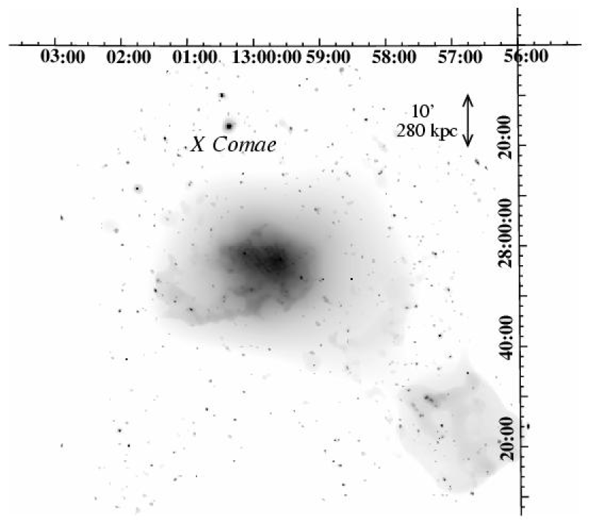
Figure 1.— An image of the Coma cluster in the 0.5–2.0 keV band from Finoguenov et al. (2003). The coordinate grid is RA, Dec (J2000.0).

Table 1 Instrument mode

Instrument	Mode	Filter
RGS	Spectro+Q	—
EPIC pn	Full frame	Medium
EPIC MOS	Full frame	Thin

Table 2 Exposure times and fluxes of X Comae

Date	Duration	Net exposure	Flux (0.3–2.0 keV)
	ks	ks   ks	$\mathrm{ergs~{}cm^{-2}~{}s^{-1}}$
2004 Jun 6	102.6	71.5  60.1	$1.92\times 10^{-12}$
2004 Jun 18	108.3	54.7  46.2	$1.48\times 10^{-12}$
2004 Jul 12	104.2	45.6  39.5	$1.36\times 10^{-12}$
2005 Jun 27	55.9	23.9  20.3	$1.02\times 10^{-12}$
2005 Jun 28	80.8	62.5  57.6	$1.46\times 10^{-12}$
Total	451.8	258.2 223.7	$1.66\times 10^{-12}$

The Coma cluster systemic redshift is $z_{\mathrm{coma}}=0.0231$ (Struble & Rood, 1999), which yields a scale of 1.68 $h_{70}^{-1}$ Mpc per degree for our assumed cosmology. The redshift dispersion of the cluster galaxies is $\sigma_{\mathrm{gal}}=3.44\times 10^{-3}$. The integrated temperature of the cluster is 8.21 keV (Hughes et al., 1993), which implies the radius within which the cluster’s average density is 200 times the critical density, $r_{200}$, is 2.4 $h^{-1}_{70}$ Mpc. At a redshift of 0.091$\pm 0.001$ (Branduardi-Raymont et al., 1985), X Comae is the brightest X-ray object behind the Coma cluster. Its position is (13^h00^m22^s.17, +28^∘24^′2^′′.6) (J2000.0). As shown in Figure 1, it is $28.4^{\prime}$ or $0.79h^{-1}_{70}$ Mpc or 0.33$r_{200}$ north of the cluster center, defined to be at NGC 4874.

We made five observations with XMM-Newton (Jansen et al., 2001) in 2004 and 2005 for a total of 451.8 ks. The instrument mode and the filter used are shown in Table 1, and the gross and net exposure times and flux of X Comae are summarized in Table 2. X Comae had a flux at or below its hitherto historical low during our observations.

3. Absorption Lines in the RGS spectra

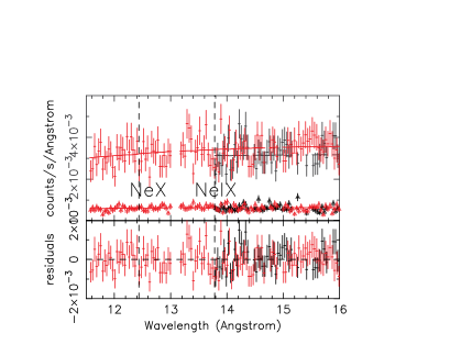
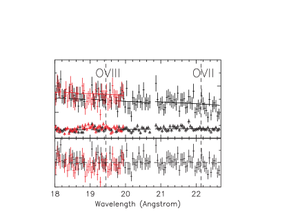
Figure 2.— (upper panel) RGS spectra around the Ne and O K$\alpha$ lines. Black and red represent RGS1 and RGS2, while crosses ($+$) and triangles ($\triangle$) show source plus background and background, respectively. The solid lines show the best fit model of source plus background and background. The wavelengths corresponding to redshifted Ne and O lines ($z=0.0231$) are indicated with vertical dashed lines. (lower panel) Source plus background residuals from the best fit broken power law model. The model is continuum only; it has no absorption features.

We reduced the RGS (den Herder et al., 2001) data using the XMM-Newton Science Analysis System (SAS) version 6.1.0, with standard parameters. We checked the data from a source-free region of CCD 9 for background flares. The regions were CHIPX = 2 to 341, CHIPY = 2 to 38 and 87 to 127 for RGS1 and CHIPX = 2 to 284, CHIPY = 2 to 37 and 87 to 127 for RGS2. We accumulated the signal photons only when the count rates in these regions were less than 0.1 s^-1 (in PI range 80 - 3000) for both RGS1 and 2. This rather severe threshold was determined empirically to yield the highest signal to noise background subtracted source spectrum. The net exposure time was about 60 % of the total exposure and is summarized in Table 2.

The spectra were extracted after merging the five data sets and then binned by a factor of four, resulting in a final bin width of 0.035 Å at 11.5 Å and 0.046 Å at 23 Å. These bin width are about half of the average FWHM wavelength resolution of the RGS (0.067 Å). The redshift widths corresponding to the resolution are 0.0058 and 0.0029 at 11.5 Å and 23 Å respectively. The background spectra were similarly produced from the same data sets using the pixels outside the region where source photons were dispersed. The background spectra were then scaled to account for the different areas used to extract source and background photons. Since the number of photons is small, we used the C-statistic (maximum-likelihood) method for model fitting. Rasmussen et al. (2006) pointed out that merging different observations may introduce artificial absorption features in RGS spectra. However, their suggested features have about one order of magnitude smaller equivalent widths than those we discuss below. They are smaller than our statistical errors. We tried the procedure to search for bad columns that may cause artificial absorptions according to their Appendix C. It showed no apparent artificial features within our statistics.

3.1. Detection of absorption features and their equivalent widths

Table 3 Results of fitting the RGS spectra of X comae with broken power law models

Component	Unit	Value
$N_{\mathrm{H}}$	cm-2	$9.3\times 10^{19}$ (fixed)
Source $\Gamma$ ($E<0.75$ keV)		$1.74^{+0.15}_{-0.29}$
Source $\Gamma$ ($E>0.75$ keV)		$2.41\pm 0.25$
Source Normalization		$(6.88^{+0.72}_{-0.66})\times 10^{-4}$
Background $\Gamma$ ($E<0.75$ keV)		$3.73^{+0.18}_{-0.12}$
Background $\Gamma$ ($E>0.75$ keV)		$1.96\pm{0.23}$
Background Normalization		$(0.79\pm 0.08)\times 10^{-4}$
C-statistic		708.63
free parameters		6
d.o.f.		628

Table 4 Ratio for continuum and absorption spectral regions

	Continuum region	Absorption region	${\it EW}$
Ne IX	$1.027\pm 0.058$	$0.782\pm 0.071~{}(98.0\%)$	$3.3\pm 1.8$ eV
Ne X	$1.011\pm 0.073$	$0.950\pm 0.092~{}(42.7\%)$	$0.8~{}(<3.9)$ eV
O VII	$0.908\pm 0.080$	$0.927\pm 0.103~{}(50.0\%)$	$0.7~{}(<2.6)$ eV
O VIII	$0.963\pm 0.054$	$0.845\pm 0.071~{}(94.1\%)$	$1.7\pm 1.3$ eV
Avg. of Ne IX and O VIII	$0.993\pm 0.039$	$0.813\pm 0.050~{}(99.7\%)$	—

Figure 3.— Ratios of the data to the continuum model (as defined in equation 1) versus $z$ for Ne IX, Ne X, O VII and O VIII (top to bottom). Vertical dashed lines indicate $z_{\mathrm{coma}}$ and $\pm 2.5\times\sigma_{\mathrm{gal}}$. The average RGS1 and RGS2 instrumental resolution of 0.067 Å (FWHM) corresponds to a redshift resolution of 0.0050, 0.0055, 0.0031 and 0.0035 (top to bottom), which is indicated as a horizontal line at the lower right of each panel.

Figure 4.— Error-weighted average ratio of the data to the continuum model (as defined in equation 1) versus $z$ for the Ne IX and O VIII lines. Vertical dashed lines indicate $z_{\mathrm{coma}}$ and $z_{\mathrm{coma}}\pm 2.5\times\sigma_{\mathrm{gal}}$. The two horizontal lines show the $\pm 1~{}\sigma$ error of the model continuum normalization with power law indices fixed at their best fit values. The average of the ratio in the six bins between the left and right vertical lines is $0.813\pm 0.050$. The significance of this absorption is 99.7% according to Monte Carlo simulations. The average of the remaining ten continuum bins is $0.993\pm 0.039$, which is consistent with unity. The FWHM averaged wavelength resolution of RGS is also shown as a horizontal line at lower right.

Figure 2 shows the RGS spectra of X Comae in the Ne region (11.5–16.0 Å) and the O region (18.0–22.7 Å). We calculated the ratio of the data to a continuum only model in order to estimate the statistical significance of possible absorption features at the wavelengths of Ne IX, Ne X, O VII and O VIII K$\alpha$ resonance lines of the Coma redshift ($z=0.0231$) in a model independent way. That is, we calculated

$${\rm Ratio}\equiv\frac{{\rm(source+background~{}data)-(background~{}data)}}{{\rm(source+background~{}model)-(background~{}model)}}.$$ (1)

This procedure is called the ratio method in what follows.

The source model is a broken power law multiplied by the Galactic absorption of $N_{\mathrm{H}}=9.3\times 10^{19}~{}\mathrm{cm^{-2}}$ (Dickey & Lockman, 1990). The background model is a different broken power law without Galactic absorption. In order to determine the continuum model, we fitted the source plus background and background spectra of RGS1 and 2 simultaneously using XSPEC version 11.3 in the wavelength region 11.5 Å–22.7 Å. Regions around the Ne IX, Ne X, O VII and O VIII K$\alpha$ lines, which are defined as $z_{\mathrm{coma}}-3~{}\sigma_{\mathrm{gal}}<z<z_{\mathrm{coma}}+3~{}\sigma_{\mathrm{gal}}$, were excluded from the fit.

The best fit model and parameters are shown in Figure 2 and in Table 3 respectively. The Ratios around Ne IX, Ne X, O VII and O VIII lines vs. $z$ are shown in Figure 3. The FWHM wavelength resolution of RGS is also shown as a horizontal line. We summed the RGS1 and 2 data where both were available. Since the mapping from wavelength to redshift is a function of wavelength, we interpolated the counts to a common redshift bin size for all four lines.

The three vertical dashed lines in Figure 3 indicate $z_{\mathrm{coma}}$ and $z_{\mathrm{coma}}\pm 2.5\times\sigma_{\mathrm{gal}}$. We defined redshifts within $z_{\mathrm{coma}}\pm 2.5\times\sigma_{\mathrm{gal}}$ as absorption and the remainder in Figure 3 as continuum, and then calculated the error-weighted average of the absorption and continuum ratios. The results are shown in Table 4. When the absorption redshift region was defined, we fixed its center to the apriori known $z_{\mathrm{coma}}$ and chose its width to maximize the Ne IX plus O VIII signal from among 2, 4, 6 or 8 binned-by-four pixels; i.e., the region was determined after a four-trial optimization.

Ne IX is the ion with the deepest absorption, and O VIII is the second deepest. The absorption ratio is below 1 for the Ne X and O VII lines as well, though they are not very significant. The continuum is always consistent with 1. This situation of strong Ne IX absorption and weak absorption by the other three lines is often observed at much higher signal to noise in interstellar medium features in the spectra of galactic X-ray sources (e.g. Yao & Wang, 2005).

To improve the signal-to-noise, we made a grand error-weighted average of the ratios for Ne IX and O VIII lines and calculated the combined significance. The result is shown in Figure 4 where the band around unity is $+0.7\%$, $-1.0\%$, the $1\sigma$ error of the model normalization with power law indices fixed at their best fit values. The average of the grand-averaged ratio are also given in Table 4.

Since the number of counts in each bin is not very high (20–30 counts/bin), we investigated the significance of the absorption using Monte Carlo simulations. We made 1000 simulated spectra with no absorption which have the same statistics and the same response function as the actual data, and then calculated the ratios with the same procedure as above. That is, we calculted the ratio for Ne IX, Ne X, O VII and O VIII lines and grand error-weighted average of the ratios of Ne IX and O VIII. This calculation was done for 2, 4, 6 and 8 binned-by-four pixels around $z_{\mathrm{coma}}$, and then we chose the most significant grand average among the four trials. The significance of the absorption in our observed RGS data can be estimated as the probability that the simultated spectra without absorption yield a smaller discrepancy from unity. The significance for the grand error-weighted average was 99.7%. We conclude that we have detected absorption by material associated with the Coma cluster with a significance of 99.7%. This significance is equivalent to $3.0\sigma$ of a Gaussian distribution. The significance of Ne IX and O VIII was 98.0% (2.3$\sigma$) and 94.1% (1.9$\sigma$), respectively.

The equivalent width ${\it EW}$ of the absorption lines can be calculated from the ratios as $(1-{\rm Ratio})\times\Delta E$, where $\Delta E$ is the energy corresponding to the width of 6 bins we used to calculate the ratios. The ${\it EW}$s for the four lines are also shown in Table  4. Assuming that the absorption lines are not saturated, the column density $N_{\mathrm{ion}}$ is calculated from ${\it EW}$ as

$$N_{\mathrm{ion}}=\frac{m_{\mathrm{e}}c(1+z)}{\pi he^{2}}\frac{{\it EW}}{f_{\mathrm{os}}},$$ (2)

or

$$N_{\mathrm{ion}}=9.11\times 10^{15}~{}\mathrm{cm^{-2}}\frac{(1+z)}{f_{\mathrm{os}}}\frac{{\it EW}}{1~{}\mathrm{eV}},$$ (3)

(Sarazin, 1989) where $f_{\mathrm{os}}$ is the oscillator strength of the transition and the other symbols have their usual meanings. We used $f_{\mathrm{os}}=0.724$ for the Ne IX, $f_{\mathrm{os}}=0.696$ for O VII, and $f_{\mathrm{os}}=0.416$ for Ne X and O VIII (Verner et al., 1996). The column densities of the four lines are then ${N_{\mathrm{NeIX}}}=4.3\pm 2.3\times 10^{16}~{}\mathrm{cm^{-2}}$, ${N_{\mathrm{NeX}}}=1.9~{}(<8.8)\times 10^{16}~{}\mathrm{cm^{-2}}$, ${N_{\mathrm{OVII}}}=0.9~{}(<3.5)\times 10^{16}~{}\mathrm{cm^{-2}}$ and ${N_{\mathrm{OVIII}}}=3.7\pm 2.8\times 10^{16}~{}\mathrm{cm^{-2}}$.

3.2. Fitting the absorption features and their equivalent widths

Figure 5.— Contour plot of $\Delta C$ as a function of $W_{\mathrm{notch}}$ (converted to redshift) and $F$ for the Ne IX line. Equivalent width is $W_{\mathrm{notch}}\times F$. The four contours are $\Delta C=$ 1.0, 2.71, 4.0 and 6.6 corresponding to 68%, 90%, 95% and 99% confidence for one interesting parameter, respectively. These also correspond to $1\sigma$, $1.6\sigma$, $2\sigma$ and $2.6\sigma$, respectively if the data were Gaussian distributed.

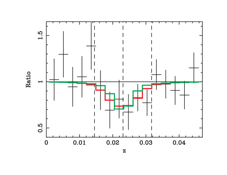
Figure 6.— Ratios of the data to the continuum model vsesus $z$ for Ne IX (the same data as the top panel of Figure 3), overlaid with boxcar absorption models. Red line shows the best-fit model, while green line displays ($F$, $W_{\mathrm{notch}}$) = (1.0, $3.1\times 10^{-3}$). Since the wavelength resolution of the RGS is comparable to the width of the absorptiion, the fit is not sensitive to $F$ or $W_{\mathrm{notch}}$ individually, but to the ${\it EW}$, which is proportional to $F\times W_{\mathrm{notch}}$. Vertical dashed lines indicate $z_{\mathrm{coma}}$ and $z_{\mathrm{coma}}\pm 2.5\times\sigma_{\mathrm{gal}}$.

Table 5Results of fitting the RGS spectra of X Comae with broken power law plus boxcar absorption models

Component	Unit	Value
Continuum
$N_{\mathrm{H}}$	$~{}\mathrm{cm^{-2}}$	$9.3\times 10^{19}$ (fixed)
Source $\Gamma$ ($E<0.75$ keV)		$1.71^{+0.21}_{-0.26}$
Source $\Gamma$ ($E>0.75$ keV)		$2.35\pm 0.24$
Source Normalization		$6.92^{+0.62}_{-0.33}\times 10^{-4}$
Background $\Gamma$ ($E>0.75$ keV)		$3.64^{+0.11}_{-0.19}$
Background $\Gamma$ ($E<0.75$ keV)		$2.01{\pm 0.21}$
Background Normalization		$(0.82\pm 0.07)\times 10^{-4}$
NeIX 13.447 Å
${\lambda_{\mathrm{notch}}}$		0.0231 (fixed)
${W_{\mathrm{notch}}}$		9.79 $\times 10^{-3}$
$F$		0.41
$EW$		3.7 ${}^{+2.0}_{-2.2}$ eV
${N_{\mathrm{ion}}}$	cm-2	4.7 ${}^{+2.6}_{-2.9}$ $\times 10^{16}$
NeX 12.134 Å
${\lambda_{\mathrm{notch}}}$		0.0231 (fixed)
${W_{\mathrm{notch}}}$		9.79 $\times 10^{-3}$ (fixed to the NeIX value)
$F$		0.09
$EW$	eV	0.8 ($<$4.7)
${N_{\mathrm{ion}}}$	cm-2	1.9 ($<$10.5) $\times 10^{16}$
${EW/EW_{\mathrm{NeIX}}}$		0.2 ($<$1.3)
${N_{\mathrm{ion}}/N_{\mathrm{NeIX}}}$		0.4 ($<$2.3)
OVII 21.602 Å
${\lambda_{\mathrm{notch}}}$		0.0231 (fixed)
${W_{\mathrm{notch}}}$		9.79 $\times 10^{-3}$ (fixed to the NeIX value)
$F$		0.04
$EW$	eV	0.2 ($<$2.2)
${N_{\mathrm{ion}}}$	cm-2	0.3 ($<$2.9) $\times 10^{16}$
${EW/EW_{\mathrm{NeIX}}}$		0.06 ($<$0.59)
${N_{\mathrm{ion}}/N_{\mathrm{NeIX}}}$		0.06 ($<$0.63)
OVIII 18.969 Å
${\lambda_{\mathrm{notch}}}$		0.0231 (fixed)
${W_{\mathrm{notch}}}$		9.79 $\times 10^{-3}$ (fixed to the NeIX value)
$F$		0.06
$EW$	eV	0.4 ($<$2.2)
${N_{\mathrm{ion}}}$	cm-2	0.8 ($<$4.9) $\times 10^{16}$
${EW/EW_{\mathrm{NeIX}}}$		0.10 ($<$0.59)
${N_{\mathrm{ion}}/N_{\mathrm{NeIX}}}$		0.2 ($<$1.0)
C-statistic		834.33
Free parameters		11
Degrees of freedom		745

Next we derived the equivalent widths of the four lines by another way: using model-fitting of the spectra. We adopted the same contimuum model as that in § 3.1, and a boxcar profile to describe the absorption (NOTCH model in XSPEC). This absorption model multiplies the continuum by a factor of

$$\left\{\small\begin{array}[]{ll}(1-F)&\quad{\rm for~{}}(\lambda_{\mathrm{notch}}-\frac{W_{\mathrm{notch}}}{2})<\lambda<(\lambda_{\mathrm{notch}}+\frac{W_{\mathrm{notch}}}{2})\\ 1&\quad{\rm for~{}all~{}other,}\end{array}\right.$$ (4)

where $\lambda_{\mathrm{notch}}$, $W_{\mathrm{notch}}$ and $F$ are the central wavelength, width and absorption factor, respectively. The equivalent width is given by ${\it EW}=W_{\mathrm{notch}}\times F$. We fixed $\lambda_{\mathrm{notch}}$ to be the value corresponding the redshift of the Coma cluster. Since the significances of the absorption features were low, except for Ne IX, we fitted the Ne IX absorption first and then fitted the other lines with $W_{\mathrm{notch}}$ fixed to the best fit Ne IX value (in $z$, not wavelength). All together the free parameters were: power law indices and normalizations of the source and background continua, $W_{\mathrm{notch}}$ and $F$ for Ne IX absorption, and $F$ for the other species. Data between 11.5–22.7 Å were used in the fit.

The best fit parameters are shown in Table 5, where $\lambda_{\mathrm{notch}}$ and $W_{\mathrm{notch}}$ are converted to redshift. The equivalent widths and their errors were determined taking into account the covariance between $W_{\mathrm{notch}}$ and $F$, as is shown in Figure 5 for Ne IX. Figure 5 indicates that this analysis is not sensitive to $F$ or $W_{\mathrm{notch}}$ because the wavelength resolution of RGS is comparable to the width of the absorption. Figure 6 compares the best-fit (red) boxcar absorption model and the model with $F=1.0$ and $W_{\mathrm{notch}}=3.1\times 10^{-3}$ (green). There is little difference between them. Note that we can estimate the ${\it EW}$, the product of $F$ and $W_{\mathrm{notch}}$, more precisely than either $F$ or $W_{\mathrm{notch}}$. From this figure, the equivalent width of Ne IX is estimated to be $3.7^{+2.0}_{-2.2}$ eV (90% confidence errors). Best fit values and 2$\sigma$ upper limits are also given in Table 5 for the Ne X, O VII and O VIII absorption lines. The column density $N_{\mathrm{ion}}$ of each ion, estimated from the ${\it EW}$ are tabulated in Table 5 as well. The derived equivalent widths are consistent within the errors with those obtained from the ratio of the data to the continuum model described in § 3.1.

The significance of the line was again calculated using Monte Carlo simulations. The C-statistic was improved by 7.57 when we added the Ne IX absorption line. The probability that the simulated data shows less improvement of the C-statistic was 99.2%, equivalent to $2.7\sigma$ if the data were Gaussian distributed (compared to 98.0% from the ratio method). We took this value as the significance of Ne IX line with boxcar-fitting. In the case of boxcar-fitting, the O VIII line is less significant than that found with the ratio method (82.4% compared to 94.1%) and hence combining Ne IX and O VIII absorption did not improve the significance (98.5%) compared to that of Ne IX alone. The significances obtained with boxcar-fitting were slightly different from those by the ratio method, particularly for O VIII. This is probably because the two methods are not exactly identical: with boxcar-fitting the detector response is convolved with an assumed absorption shape (boxcar) that is same for the four lines, while no shape was assumed for the ratio method.

4. Emission Lines in the EPIC Spectra

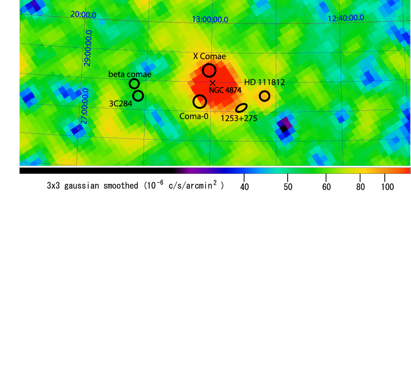
Figure 7.— ROSAT R4 band map ($\sim$0.4–1.0 keV) near the Coma cluster (Snowden et al., 1997) with analyzed regions of the EPIC overlaid. The R4 band map was smoothed with a two-dimensional Gaussian with $\sigma$ = 3 pixels.

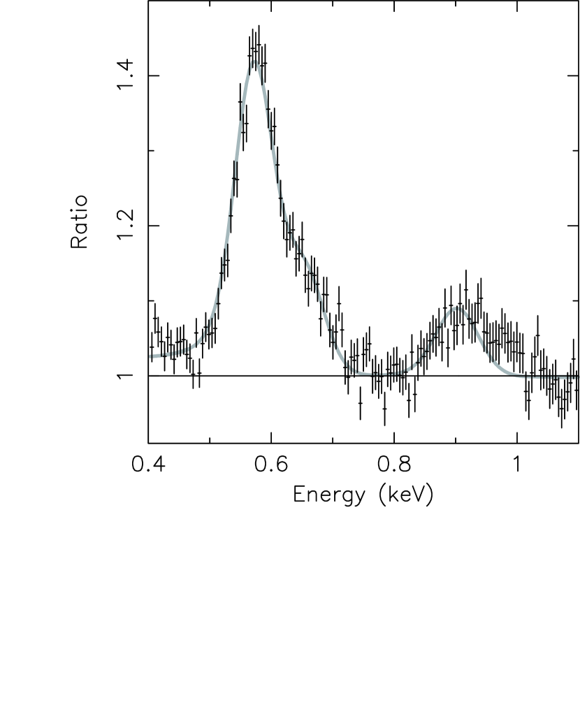
Figure 8.— EPIC pn spectrum from the entire X Comae field. Plotted is the ratio of the data to the smooth continuum with parameters in Table 7. The grey line is a fit of three narrow width Gaussians to the residuals. The centers of the lower-energy Gaussians are fixed to O VII and O VIII at zero redshift and that of the higher-energy Gaussian is fixed to Ne IX at the Coma redshift.

Figure 9.— Surface brightness of O VII and O VIII (crosses ($+$) and triangles ($\vartriangle$), divided by ten) and Ne IX (circles ($\circ$)) versus distance from NGC 4874, which we take as the center of the Coma cluster.

Table 6O and Ne line intensity

Field	ObsID	Exp.	Distance from	O VII $I$	O VIII $I$	NeIX $I$
			NGC 4874
		ks	arcmin
X Comae			26.5	$55.6^{+2.1}_{-1.8}$	$15.4^{+1.3}_{-1.4}$	$6.0\pm 0.9$
X Comae 1			17.6	$61.7^{-12.8}_{-13.5}$	$12.9^{+9.2}_{-10.7}$	$11.5^{+6.4}_{-8.4}$
X Comae 2			20.6	$59.7^{-5.8}_{-5.5}$	$14.8^{+4.2}_{-3.9}$	$7.7^{+2.8}_{-2.7}$
X Comae 3			25.9	$54.7^{-3.7}_{-3.5}$	$15.0^{+2.4}_{-2.5}$	$5.7\pm 1.7$
X Comae 4			31.8	$53.5^{-2.8}_{-3.1}$	$16.0\pm 2.1$	$3.8^{+1.4}_{-1.3}$
X Comae 5			38.2	$53.2^{+4.1}_{-4.0}$	$15.6^{+2.7}_{-2.8}$	$5.2^{+1.7}_{-1.8}$
Coma 0	0124711501	15.4	46.2	$71.5\pm 5.1$	$28.1\pm 3.4$	$4.5\pm 1.8$
1253+275	0058940701	10.5	71.6	$44.9^{+6.5}_{-6.7}$	$15.1\pm 4.5$	$1.1~{}(<3.9)$
3C 284	0021740201	34.2	156.4	$62.2\pm 4.0$	$26.4\pm 2.5$	$3.7\pm 1.2$
$\beta$ Comae	0148680101	29.4	162.7	$70.2\pm 5.5$	$17.5\pm 3.2$	$3.7\pm 1.6$
Average bkgd			109.2	$62.2\pm 9.8$	$21.8\pm 5.2$	$3.3\pm 1.2$
Average bkgd			130.2	$59.1\pm 12.0$	$19.7\pm 5.5$	$2.8\pm 1.4$
Wtd avg bkgd			109.2	$63.6\pm 2.5$	$23.1\pm 1.6$	$3.5\pm 0.8$
Wtd avg bkgd			130.2	$61.1\pm 2.9$	$21.8\pm 1.8$	$3.3\pm 0.9$

We cleaned the EPIC X Comae data of flares as described by Finoguenov et al. (2003). This procedure yielded 223.7 ks of clean EPIC pn (Strüder et al., 2001) data. This exposure is among the longest ever made of a cluster with XMM-Newton. We considered the entire X Comae field, as well as dividing it into five concentric sectors of annuli, approximately centered on the center of the cluster.

Determining a reliable background is crucial for this work because the temperatures of the WHIM and the Milky Way interstellar medium are similar and the soft emission in the X Comae field is not very bright. Many previous attempts to measure the soft emission from the Coma cluster (e.g. Finoguenov et al., 2003; Kaastra et al., 2003) used ROSAT All-Sky Survey (RASS) data to obtain the values of the components of a galactic background model. The resulting background subtraction is only as good as the model. Since then there have been several XMM-Newton observations serendipitously located around the Coma cluster, as we show in Figure 7. Those observations provide a true background measured with the same instrument as our data and are therefore preferable for our analysis. We have examined the RASS data at the location of these fields to determine whether they are representative of the general background around the Coma cluster. One of them, HD111812 (ObsID 0008220201), was located on an unusually bright spot of the RASS maps and has been omitted from the analysis. Some properties of the four remaining fields are shown in Table 6.

We performed the following analysis on these ten fields. We excised point sources including X Comae. We also excised diffuse sources using a wavelet-based detection algorithm, which were on a spatial scale of 4″  to 4′  and had a surface brightness comparable to that of the cluster emission. We extracted a spectrum from each of the ten fields and subtracted a filter wheel closed accumulation from each. We determined the vignetting correction assuming a uniform source surface brightness in each field. We fitted the net vignetting corrected spectrum with a collisionally ionized thermal plasma model component (APEC in XSPEC) for the Coma hot gas, (except for the two background fields most distant from the Coma center), plus an APEC component for the Milky Way background, plus a power law component for the cosmic X-ray background. The free and fixed parameters of the models are given in Table 7. The energy range for the spectral fit was 0.4-7.0 keV, excluding the energies of strong detector lines (1.4–1.6 keV). We used the improved response matrix from the SAS v6.5 calibration release. Our key finding is a clear detection of O VII, O VIII and Ne IX lines in excess of the continuum for the entire X Comae field, as shown in Figure 8. Although there still remain small residuals at 0.97 keV, which might be identified as Fe XX L line complex, the statistical significance of this feature is not high and hence we will not discuss it further.

We then fitted narrow Gaussians at the energies of the O VII, O VIII and Ne IX lines. The results are in Figure 8 and Table 7 for the entire X Comae field and Figure 9 and Table 6 for the other fields. The intensity of the Ne IX component increases towards the Coma cluster center (see Figure 9) and its intensity in the sector nearest the position of X Comae is above that of the background fields. The Coma intracluster medium is too hot to produce this line. We can also rule out a solar wind origin, as no variation with respect to the center of the Coma cluster in a single pointing is expected for that scenario. We thus conclude that we have detected Ne IX line emission from Coma cluster material that is cooler than most of the Coma intracluster medium.

The intensity of the O VII and O VIII Gaussian components did not vary in an obvious way as a function of position (see Figure 9). The two oxygen lines show no enhancement at the position of the cluster: their intensity in the five X Comae sectors is the same or even lower than that in the background fields. We thus conclude that all of the oxygen emission comes from the Milky Way soft background and not from material in the Coma cluster.

The intensity of O VII and O VIII lines has a large scatter from one background field to another. The intensity in one of them (the 1253+275 field) is consistent with the soft X-ray background measured by McCammon et al. (2002) (they obtained $40.6\pm 10.9$ and $13.5\pm 5.4$ $\times 10^{-8}~{}\mathrm{ph~{}cm^{-2}~{}s^{-1}~{}arcmin^{-2}}$, for O VII and O VIII, respectively), while the intensity in the other fields are larger than their values. On the other hand, the scatter of the Ne IX intensity among the background fields is not as large and the average is consistent with the upper limit of McCammon et al. (2002). ($<5.4\times 10^{-8}~{}\mathrm{ph~{}cm^{-2}~{}s^{-1}~{}arcmin^{-2}}$, from their Figure 13).

Do we expect not to be able to detect Coma cluster oxygen emission given the strength of the cluster neon line? The O VII surface brightness is 1.67 times that of Ne IX, for a temperature of $4\times 10^{6}$ K and a Ne/O number density ratio of 0.14 (see § 5.1.1 for a justification of these values). This expected O VII line intensity in the entire X Comae field is approximately the dispersion of the other nine measurements (10.0 versus 8.0 $\times 10^{-8}$ ph cm^-2 s^-1 arcmin^-2, respectively). Thus the different behavior of the neon and oxygen emission lines is probably due to the much lower galactic neon background intensity that allows the Coma neon emission to be detected. The higher galactic oxygen background intensity masks the Coma oxygen emission in the X Comae fields.

In the next section we will need the net Ne IX intensity at the position of X Comae. Of course this measurement requires an extrapolation to that position since the glare from the AGN prevents measurement of emission from the Coma cluster gas. We give in Table 6 the numerical and error-weighted average of all four background fields and the three fields excluding Coma 0. The numerical average is more appropriate if there are real variations from field to field. Excluding Coma 0 is appropriate if it has a higher intensity. Since none of the four averages are statistically distinguishable, we take for the Ne IX background the weighted average of all background fields since it has the lowest error. Similarly we take for the gross intensity the value from the entire X Comae field, since it is statistically indistinguishable from the sector closest to X Comae but has a lower error. The net intensity is thus $2.5\pm 1.2\times 10^{-8}~{}\mathrm{ph~{}cm^{-2}~{}s^{-1}~{}arcmin^{-2}}$ (90% confidence errors or $3.4\sigma$ detection).

The intensity of Ne IX line is only 9% of the continuum level, as is seen in Figure  8. Such a low intensity may mean that its measurement is subject to systematic errors in the continuum. We therefore repeated the entire preceding analysis with six additional continuum models that froze or thawed different components and/or added a soft proton component that was not folded through the mirror area. The dispersion in the seven measurement of the net Ne IX intensity was less than the above statistical error. We conclude that the statistical error accurately reflects the uncertainties of the measurement.

Table 7 Results of fitting the EPIC pn spectrum of diffuse gas at the position of X Comae

Component	Unit	Value
Galactic absorption
$N_{\mathrm{H}}$	$~{}\mathrm{cm^{-2}}$	$8.0\times 10^{19}$ (fixed)
Coma hot ICM
$kT$	keV	$3.75^{+0.32}_{-0.50}$
Abundance	solar	$0.47\pm 0.09$
z		0.0231 (fixed)
Normalization		$7.77^{+0.70}_{-0.85}\times 10^{-6}$
Milky Way warm ISM
$kT$	keV	$0.174^{+0.002}_{-0.001}$
Abundance	solar	0, 1 (fixed)
z		0 (fixed)
Normalization		$5.5\pm{0.2}\times 10^{-6}$
Cosmic X-ray Background
$\Gamma$		$1.40$ (fixed)
Normalization		$4.05^{+0.23}_{-0.18}\times 10^{-4}$
O VII emission line
$E$	keV	0.574 (fixed)
$I$		$55.6^{+2.1}_{-1.8}\times 10^{-8}$
O VIII emission line
$E$	keV	0.654 (fixed)
$I$		$15.4^{+1.3}_{-1.4}\times 10^{-8}$
Ne IX emission line
$E$		0.901 (fixed)
$I$		$6.0\pm 0.9\times 10^{-8}$
Chi-squared		1305.15
Free parameters		9
Degrees of freedom		1272

5. Discussion

5.1. Properties of the warm-hot gas

We have detected absorption features in the RGS spectra of X Comae at the redshift of the Coma cluster with a combined confidence of 99.7% (equivalent to $3.0\sigma$ of a Gaussian distribution) and line emission features in the EPIC pn spectra of diffuse gas at the position of X Comae at the $3.4\sigma$ confidence level. Although the significance of either one is not very high, the fact that we observed both absorption and emission from Ne IX at the Coma cluster redshift or position is additional support for the detection of this ion. In this section we give the properties of the warm-hot gas that can be deduced from our observations under the assumption that the absorbing and emitting materials are the same and that material is uniformly distributed in a single phase in collisional ionization equilibrium. Although these assumptions have the virtue that they are simple and are consistent with the observations, it is entirely possible, even likely, that the actual situation is more complicated. In this case the properties we derive will be typical of the dominant phase of the material.

5.1.1 Temperature and Ne/O number density ratio

Figure 10.— The ratio of the theoretically expected ${\it EW}$s of Ne X, O VII or O VIII to Ne IX divided by the observed upper limits to that ratio. The dotted line shows NeX, while the dashed lines show the larger value for OVII or OVIII. Since the theoretical OVII or OVIII to NeIX ${\it EW}$ ratios depend on the number density ratio of Ne/O, we indicate three cases: 0.14 as the canonical value, 0.41 as the highest one found from literature, and 0.82 as the extremely high Ne/O case. The allowed temperature is the range in which both NeIX and O curves are below 1. There is no allowed temperature range for Ne/O = 0.14, while it is $2.0\times 10^{6}~{}\mathrm{K}<T<5.8\times 10^{6}~{}\mathrm{K}$ for the extremely high Ne/O case. The ionization fraction given in Table 2 and 3 of Chen et al. (2003) for collisional ionization case was assumed.

Figure 11.— (left) Equivalent width ratio as a function of temperature $T$, based on Figure 2 and 3 of Chen et al. (2003) in the collisional ionization equilibrium case. Solid and dashed curves correspond to OVII/OVIII and NeX/NeIX, respectively. The horizontal lines represent the upper limits determined by this work. The allowed temperature is that for which the curved lines are below the horizontal upper limit lines of the same style, i.e., $T>2.2\times 10^{6}$ K for OVII/OVIII and $T<5.7\times 10^{6}$ K for NeX/NeIX. (right) Ne/O number density ratio as a function of temperature $T$. The three curves correspond to the best-fit values and $\pm 1\sigma$ errors, respectively, obtained from the observed Ne IX/O VIII ratio.

We can constrain the temperature of a plasma in ionization equilibrium from the ratios of absorption ${\it EW}$s between different ionization states of the same species. On the other hand, we can constrain the number density (or abundance) ratio of different elements from the ratio of absorption ${\it EW}$s between lines of different species.

First, we investigate the allowed temperature and abundance for the boxcar-fitting case. Figure 10 plots the ratio of the theoretically expected ${\it EW}$s of Ne X, O VII or O VIII to Ne IX divided by the observed upper limits to that ratio. That is, it plots a ratio of ratios. The expected values were calculated using the ionization fractions of a plasma under collisional ionization equilibrium given in Figures 2 and 3 of Chen et al. (2003). In this calculation we assumed ${\it EW}\propto N_{\mathrm{ion}}f_{\mathrm{os}}$, i.e. no saturation. The dotted line shows Ne X, while the dashed lines show the larger value for O VII or O VIII. The allowed temperature is the range for which both the Ne IX and O curves are below 1. The upper limit of Ne X/Ne IX ratio gives a robust upper limit of the temperature, $T<5.8\times 10^{6}$ K.

The theoretical O VII or O VIII to Ne IX ${\it EW}$ ratios depend on the number density ratio of Ne/O, while Ne/O ratio is not well known even for solar or interstellar values. The widely-used solar Ne/O number density ratio is 0.14 (Anders & Grevesse, 1989). However it is difficult to measure the abundance of Ne due to its absence in the solar photospheric spectrum or in meteorites. Further, the O abundance also contains uncertainties; improved modeling of solar photosphere lines has yielded lower abundances for some elements including O and Ne (Asplund et al., 2005). Recent measurements using coronal X-ray or quiet Sun EUV lines find Ne/O $<$ 0.30 (95% confidence) or 0.17$\pm$0.05 (estimated systematic errors) respectively (Schmelz et al., 2005; Young, 2005). A higher Ne/O ratio, 0.41, was suggested by X-ray spectroscopy of mostly giant stars and multiple systems (Drake & Testa, 2005). Recent measurements of sightlines to 4U1820-303 and LMC X-3 through the interstellar medium yield $0.20^{+0.10}_{-0.07}$ (90% confidence) and $>$0.14 (95% confidence) respectively (Yao & Wang, 2006; Wang et al., 2005). Thus the situation is not yet clear with reported values ranging from 0.14 to 0.41.

Since our boxcar-fitting cannot determine the Ne/O ratio, we indicate three cases in Figure 10: 0.14 as the canonical value, 0.41 as the highest one found in the literature, and 0.82 as an extremely high Ne/O case. We found that Ne/O $>0.25$ (2$\sigma$) is necessary in order to reproduce the boxcar-fit results with an assumption of single temperature plasma; for example, there is no intersection of O curve and 1 for Ne/O = 0.14. Thus, the canonical Ne/O ratio (Ne/O = 0.14) is rejected in this analysis. On the other hand, if Ne/O was larger than 0.25, there was allowed temperature range. Even if adopting an extremely high Ne/O ratio, Ne/O = 0.82, the temperature range can be constrained to be $T>2.0\times 10^{6}~{}\mathrm{K}$. Combining this constraint with that from Ne X/Ne IX ratio, we obtained a conservative temperature range, $2.0\times 10^{6}~{}\mathrm{K}<T<5.8\times 10^{6}~{}\mathrm{K}$.

We next used the ${\it EW}$s determined with the ratio method (§ 3.1). This method is independent of the intrinsic shape of the absorption. The left panel of Figure 11 shows the theoretical equivalent width ratios of O VII/O VIII and Ne X/Ne IX as a function of temperature $T$ again based on Figures 2 and 3 of Chen et al. (2003) in the case of collisional ionization equilibrium. Note that here we use the O VII/O VIII ratio because O VIII was also detected at more than 90% confidence with the ratio method. We show the observed 2$\sigma$ upper limits obtained in § 3.1 with horizontal lines in the left panel of Figure 11. The allowed temperature range is that for which the curved lines are below the horizontal upper limits of that ratio, i.e., $T>2.2\times 10^{6}$ K for O VII/O VIII and $T<5.7\times 10^{6}$ K for Ne IX/Ne X. Combining these two constraints, we restricted the temperature of the plasma to be $2.2\times 10^{6}~{}\mathrm{K}<T<5.7\times 10^{6}~{}\mathrm{K}$ at the 2$\sigma$ confidence level.

From the Ne IX/O VIII ratio, we can investigate the allowed Ne/O number density ratio as a function of temperature $T$. This is shown in the right panel of Figure 11. The $\pm 1\sigma$ error range is also shown. The allowed Ne/O ratio is not very sensitive to temperature; it is roughly $0.3\pm 0.15$ to $0.5\pm 0.3$ within the allowed temperature range found above. Although our best-fit Ne/O ratio suggests a Ne overabundance, all of the above including the canonical value of 0.14 is within our $\sim 1\sigma$ confidence limit. Note that both temperature range and Ne/O ratio are consistent in the two estimates (boxcar fitting and ratio values).

5.1.2 Density, line of sight length and metallicity

Figure 12.— Derived $n_{\mathrm{H}}$ (upper) and $ZL$ (lower) as a function of $T$. Solid and dashed curves represents best-fit values and $1\sigma$ confidence regions, respectively. Vertical dotted lines indicate allowed temperature range, $2.0\times 10^{6}~{}\mathrm{K}<T<5.8\times 10^{6}~{}\mathrm{K}$ (see Figure 11).

We can constrain the average hydrogen density $n_{\mathrm{H}}$ of the warm-hot gas and its path length $L$ along the line of sight by combining absorption and emission observations of the same ion, Ne IX in our case. The column density of an ion is

$$N_{\mathrm{ion}}=f_{\mathrm{ion}}Zn_{\mathrm{H}}L$$ (5)

where $Z$ is the abundance of the element relative to hydrogen. Equation (2) gives $N_{ion}$ as a function of the observed $EW$. The surface brightness of an emission line $I$ is

$$I=\frac{C}{(1+z)^{3}}Zn_{\mathrm{H}}^{2}L$$ (6)

where the exponent of $(1+z)$ is three instead of four because we measure surface brightness in photons, not ergs, and $C$ is a coefficient depending on temperature but not on the elemental abundance. Solving these two equations simultaneously gives

$$n_{\mathrm{H}}=\frac{f_{\mathrm{ion}}(1+z)^{3}}{C}\frac{I}{N_{\mathrm{ion}}}$$ (7)

and

$$ZL=\frac{C}{f_{\mathrm{ion}}^{2}(1+z)^{3}}\frac{N_{\mathrm{ion}}^{2}}{I}$$ (8)

.

The coefficient $C$ is

$$C=\frac{1}{4\pi}\left(\frac{n_{\mathrm{e}}}{n_{\mathrm{H}}}\right)^{2}\frac{1}{Z(M)}\sum_{j}\frac{P^{\prime}_{j}}{E_{j}}.$$ (9)

Here $n_{\mathrm{e}}/n_{\mathrm{H}}=1.17$, $Z(M)$ is the abundance of the element assumed by Mewe et al. (1985) ($8.32\times 10^{-5}$ for neon), $P^{\prime}$ is tabulated in Table IV of Mewe et al. (1985), $E$ is the energy of the line and the sum is over all lines not resolved with CCD energy resolution. For the Ne IX emission $C$ comes from six lines: Ne IX resonance line (13.44 Å), three satellite lines of Ne VIII (13.44 Å, 13.46 Å and 13.55 Å), Ne IX intercombination line (13.55 Å) and Ne IX forbidden line (13.70 Å).

We derive the parameters of the material producing the Ne IX absorption and emission as a function of temperature from its column density and intensity at the position of X Comae found at the ends of Sections 3.2 and 4, respectively. For example, a temperature of $4.0\times 10^{6}$ K gives $C=5.37\times 10^{-13}~{}\mathrm{photons~{}cm^{3}~{}s^{-1}~{}sr^{-1}}$ and $f_{\mathrm{ion}}=0.50$. Then

$$n_{\mathrm{H}}=6.1\times 10^{-6}~{}{\rm cm}^{-3}\left(\frac{I}{2.5\times 10^{-8}}\right)\left(\frac{N_{\mathrm{NeIX}}}{4.4\times 10^{16}~{}{\rm cm}^{-2}}\right)^{-1},\qquad$$ (10)

$$(Z/Z_{\odot})L=41~{}{\rm Mpc}\left(\frac{I}{2.5\times 10^{-8}}\right)^{-1}\left(\frac{N_{\mathrm{NeIX}}}{4.4\times 10^{16}~{}{\rm cm}^{-2}}\right)^{2},$$ (11)

where $Z_{\odot}=1.23\times 10^{-4}$ is the solar abundance of Ne relative to H (Anders & Grevesse, 1989). The derived values of $n_{\mathrm{H}}$ and $ZL$ depend strongly on the temperature. We show in Figure 12 the values as a function of temperature, where solid and dashed curves represent best-fit values and $1\sigma$ confidence regions, respectively. Vertical dotted lines indicate the allowed temperature range, $2.0\times 10^{6}~{}\mathrm{K}<T<5.8\times 10^{6}~{}\mathrm{K}$ (see Figure 10). We constrained $n_{\mathrm{H}}$ to be $2\times 10^{-6}~{}\mathrm{cm^{-3}}<n_{\mathrm{H}}<8\times 10^{-5}~{}\mathrm{cm^{-3}}$ and $ZL$ to be $1~{}Z_{\odot}\mathrm{Mpc}<ZL<300~{}Z_{\odot}\mathrm{Mpc}$. These limits are at approximately the $3\sigma$ confidence level since they sum the $2\sigma$ limit on temperature and the $1\sigma$ limit on $n_{\mathrm{H}}$ and $ZL$ (i.e., do not sum the errors in quadrature). The derived hydrogen density corresponds to $10<\delta<400$. Here $\delta$ is the overdensity with respect to the mean density of the universe: $\delta\equiv n_{\mathrm{H}}/\bar{n_{\mathrm{H}}}$ with $\bar{n_{\mathrm{H}}}=X\Omega_{b}\rho_{c}(1+z)^{3}/m_{\mathrm{H}}$. $X=0.71$ is the hydrogen-to-baryon mass ratio and $\Omega_{b}=0.0224h^{-2}$ is the baryon density relative to the critical density $\rho_{c}$.

Although the constraint we obtained on $ZL$ is not tight, we note that the lower limit on $L$ is $>1~{}\mathrm{Mpc}~{}(Z/Z_{\odot})^{-1}$. The measured value of $Z/Z_{\odot}$ at the position of X Comae is 0.16$\pm$0.05 (68% confidence error) for iron (De Grandi & Molendi, 2001), where $Z_{\odot}=4.68\times 10^{-5}$ is the solar abundance of iron (Anders & Grevesse, 1989). Thus, the scale of the plasma that contains Ne IX is at least 2.6 times the size of the Coma cluster ($r_{200}=2.4h^{-1}_{70}$ Mpc) if the Ne and Fe abundances are approximately the same. For at least two clusters (2A 0335+096 and Sérsic 159–03) RGS observations show that the Ne/Fe is approximately unity or slightly less (Werner et al., 2006; de Plaa et al., 2006). We conclude that the material containing Ne IX is likely not in the Coma cluster.

5.2. Can the Ne IX emission come from material within the cluster virial radius?

We investigate the suggestion by Cheng et al. (2005) that gas associated with merging sub-groups inside the cluster virial region, which preserves its identity for a while before being destroyed by the hot intracluster medium, is responsible for the cluster soft excess. In particular, we determine whether this material can produce the Ne IX emission we observe. We disregard the constraints from the absorption measurements here. Rather we assume that the temperature of this material is $2\times 10^{6}$ K, the peak of the Ne IX ion fraction, and that the material is in pressure equilibrium with the ICM. Neither of these assumptions is very constraining. Changing the temperature to $4\times 10^{6}$ K, the midpoint of the allowed range found previously, changes the results calculated below by less than a factor of two. The second assumption yields a density of warm-hot material similar to the densest regions of groups, which we could have assumed at the outset since that is the suggestion we are investigating.

First we need the properties of the hot ICM. The emission-weighted temperature at the position of X Comae is 7.4 keV from the temperature map of Honda et al. (1996). The emission measure-weighted hydrogen density at the position of X Comae is $2\times 10^{-4}h^{1/2}_{70}$ cm^-3 (Briel et al., 1992). Next we need the properties of the warm-hot material. A temperature of 0.172 keV and pressure equilibrium with the ICM yields a hydrogen density of $8.6\times 10^{-3}h^{1/2}_{70}$ cm^-3, or $\delta\sim 3.4\times 10^{4}$, and entropy $\sim 4$ keV $h^{-1/3}_{70}$ cm². The latter two values place the warm-hot material on the extreme high density tail of the phase plot in Figure 4 of Cheng et al. (2005). Equation (8) with C($2\times 10^{6}$ K) = $1.19\times 10^{-13}~{}\mathrm{photons~{}cm^{3}~{}s^{-1}~{}sr^{-1}}$, the above hydrogen density and the observed Ne IX surface brightness imply the path length through the material $L$ is $\sim 100$ pc. The sound crossing time across $L$ is $\sim 5\times 10^{5}$ years, during which the material travels $\sim 600$ pc moving at $\sigma_{gal}~{}c$. Thus pressure equilibrium is a good assumption because the ICM pressure hardly changes over such a small distance.

How long can this warm-hot material survive? We assume its size across the line of sight is also $L$, that is the warm-hot material is tiny blobs of diameter $\sim 100$ pc. Following Cowie & McKee (1977), the classical heat conduction across the blob-cluster interface is saturated. The saturated evaporation time is $\sim 1\times 10^{4}$ years, from their equation (64). Any blobs that might exist are very quickly destroyed. Further they are not replenished since the time for group gas at a temperature of 2 keV and the above density to cool to a temperature at which there is a significant population of Ne IX is $\sim 5\times 10^{10}$ years.

Even after the blobs evaporate it takes some additional time for the Ne ion distribution to equilibrate to that appropriate to the new temperature in which the Ne finds itself. The longest lived ion capable of emitting the Ne IX resonace line we detect is Ne X, which it does by electron capture to an excited level followed by radiative deexcitation. The ionization time $\tau_{\mathrm{ion}}$ to convert Ne X to Ne XI is mostly determined by the collisional ionization efficiency $S_{\mathrm{NeX}}$; i.e., $\tau_{\mathrm{ion}}\sim 1/n_{\mathrm{e}}S_{\mathrm{NeX}}$. The recombination rate is negligibly small and the ionization time to convert Ne IX to Ne X is smaller than that for Ne X to Ne XI in our case. The empirical formula for $S_{\mathrm{NeX}}$ for coronal plasma is given in McWhirter (1965, equation 40 of Chapter 5) as

$$S_{\mathrm{NeX}}=1.10\times 10^{-5}\frac{(kT_{\mathrm{e}}/\chi)^{1/2}}{\chi^{3/2}~{}(6+kT_{\mathrm{e}}/\chi)}~{}\exp\left(-\frac{\chi}{kT_{\mathrm{e}}}\right)~{}\mathrm{cm^{-3}~{}s^{-1}},$$ (12)

where $T_{\mathrm{e}}$ and $\chi$ are the electron temperature and the ionization energy in eV, respectively. Substituting the properties of the hot gas, $T_{\mathrm{e}}=7400$ eV, $\chi=1360$ eV, and $n_{\mathrm{e}}=2.3\times 10^{-4}~{}\mathrm{h^{1/2}_{70}cm^{-3}}$, we find $\tau_{\mathrm{ion}}=3.7\times 10^{6}$ years. The evaporation and the equilibration times are much smaller than the cluster crossing time, the characteristic scale of the situation. Thus we conclude that, under reasonable assumptions, material within the cluster virial radius is not capable of producing the observed Ne IX emission unless we are viewing the Coma cluster at a very special epoch.

6. Summary

Our main result is the detection of absorption and emission lines from Ne IX associated with the Coma cluster of galaxies. The absorption is centered on the previously known Coma redshift, although it is of marginal statistical significance ($98.0\%$ to $99.2\%$ confidence depending on the analysis method). The emission is statistically significant ($3.4\sigma$) and is positionally coincident with Coma. While the absorption line is resolved, its width is much smaller than the spectral resolution of the emission line data. We do not know if the emission and absorption lines have the same profile. The properties of material causing these lines, assuming it is in a single phase in collisioinal ionization equilibrium, are constrained as follows: temperature $T$ is $2.0\times 10^{6}~{}\mathrm{K}<T<5.8\times 10^{6}~{}\mathrm{K}$, density $n_{\mathrm{H}}$ is $2\times 10^{-6}~{}\mathrm{cm^{-3}}<n_{\mathrm{H}}<8\times 10^{-5}~{}\mathrm{cm^{-3}}$, overdensity $\delta$ is $10<\delta<400$, line of sight path length through it is $L>6~{}\mathrm{Mpc}~{}(Z/0.16~{}Z_{\odot})^{-1}$.

These properties are similar to those expected of the warm-hot intergalactic medium and we conclude that we have detected it. The warm-hot intergalactic medium is also expected to be distributed in filaments connecting clusters of galaxies. Since X Comae lies behind the apparent continuation of the Coma-A1367 chain of galaxies to the northeast of the Coma cluster (Gavazzi et al., 1999), the material we detect may reside in this previously identified filament.

References

- Anders & Grevesse (1989) Anders, E., & Grevesse, N. 1989, Geochim. Cosmochim. Acta, 53, 197
- Asplund et al. (2005) Asplund, M., Grevesse, N., & Sauval, A. J. 2005, in ASP Conf. Ser. 336: Cosmic Abundances as Records of Stellar Evolution and Nucleosynthesis, 25–+
- Bonamente et al. (2002) Bonamente, M., Lieu, R., & Joy, Marshall K.and Nevalainen, J. H. 2002, ApJ, 576, 688
- Borgani et al. (2005) Borgani, S., Finoguenov, A., Kay, S. T., Ponman, T. J., Springel, V., Tozzi, P., & Voit, G. M. 2005, MNRAS, 361, 233
- Borgani et al. (2002) Borgani, S., Governato, F., Wadsley, J., Menci, N., Tozzi, P., Quinn, T., Stadel, J., & Lake, G. 2002, MNRAS, 336, 409
- Bowyer et al. (1999) Bowyer, S., Berghöfer, T. W., & Korpela, E. J. 1999, ApJ, 526, 592
- Branduardi-Raymont et al. (1985) Branduardi-Raymont, G., Mason, K. O., Murdin, P. G., & Martin, C. 1985, MNRAS, 216, 1043
- Briel et al. (1992) Briel, U. G., Henry, J. P., & Boehringer, H. 1992, A&A, 259, L31
- Cen & Ostriker (1999) Cen, R., & Ostriker, J. P. 1999, ApJ, 514, 1
- Chen et al. (2003) Chen, X., Weinberg, D. H., Katz, N., & Davé, R. 2003, ApJ, 594, 42
- Cheng et al. (2005) Cheng, L.-M., Borgani, S., Tozzi, P., Tornatore, L., Diaferio, A., Dolag, K., He, X.-T., Moscardini, L., Murante, G., & Tormen, G. 2005, A&A, 431, 405
- Cowie & McKee (1977) Cowie, L. L., & McKee, C. F. 1977, ApJ, 211, 135
- Davé et al. (2001) Davé, R., Cen, R., Ostriker, J. P., Bryan, G. L., Hernquist, L., Katz, N., Weinberg, D. H., Norman, M. L., & O’Shea, B. 2001, ApJ, 552, 473
- De Grandi & Molendi (2001) De Grandi, S., & Molendi, S. 2001, ApJ, 551, 153
- de Plaa et al. (2006) de Plaa, J., Werner, N., Bykov, A. M., Kaastra, J. S., Méndez, M., Vink, J., Bleeker, J. A. M., Bonamente, M., & Peterson, J. R. 2006, A&A, 452, 397
- den Herder et al. (2001) den Herder, J. W., Brinkman, A. C., Kahn, S. M., Branduardi-Raymont, G., Thomsen, K., Aarts, H., Audard, M., Bixler, J. V., den Boggende, A. J., Cottam, J., Decker, T., Dubbeldam, L., Erd, C., Goulooze, H., Güdel, M., Guttridge, P., Hailey, C. J., Janabi, K. A., Kaastra, J. S., de Korte, P. A. J., van Leeuwen, B. J., Mauche, C., McCalden, A. J., Mewe, R., Naber, A., Paerels, F. B., Peterson, J. R., Rasmussen, A. P., Rees, K., Sakelliou, I., Sako, M., Spodek, J., Stern, M., Tamura, T., Tandy, J., de Vries, C. P., Welch, S., & Zehnder, A. 2001, A&A, 365, L7
- Dickey & Lockman (1990) Dickey, J. M., & Lockman, F. J. 1990, ARAA, 28, 215
- Dos Santos & Doré (2002) Dos Santos, S., & Doré, O. 2002, A&A, 383, 450
- Drake & Testa (2005) Drake, J. J., & Testa, P. 2005, Nature, 436, 525
- Fang et al. (2002) Fang, T., Marshall, H. L., Lee, J. C., Davis, D. S., & Canizares, C. R. 2002, ApJ, 572, L127
- Fang et al. (2003) Fang, T., Sembach, K. R., & Canizares, C. R. 2003, ApJ, 586, L49
- Finoguenov et al. (2003) Finoguenov, A., Briel, U. G., & Henry, J. P. 2003, A&A, 410, 777
- Fujimoto et al. (2004) Fujimoto, R., Takei, Y., Tamura, T., Mitsuda, K., Yamasaki, N. Y., Shibata, R., Ohashi, T., Ota, N., Audley, Michael D.and Kelley, R. L., & Kilbourne, C. A. 2004, PASJ, 56, L29
- Futamoto et al. (2004) Futamoto, K., Mitsuda, K., Takei, Y., Fujimoto, R., & Yamasaki, N. Y. 2004, ApJ, 605, 793
- Gavazzi et al. (1999) Gavazzi, G., Carrasco, L., & Galli, R. 1999, A&AS, 136, 227
- Honda et al. (1996) Honda, H., Hirayama, M., Watanabe, M., Kunieda, H., Tawara, Y., Yamashita, K., Ohashi, T., Hughes, J. P., & Henry, J. P. 1996, ApJ, 473, L71+
- Hughes et al. (1993) Hughes, J. P., Butcher, J. A., Stewart, G. C., & Tanaka, Y. 1993, ApJ, 404, 611
- Jansen et al. (2001) Jansen, F., Lumb, D., Altieri, B., Clavel, J., Ehle, M., Erd, C., Gabriel, C., Guainazzi, M., Gondoin, P., Much, R., Munoz, R., Santos, M., Schartel, N., Texier, D., & Vacanti, G. 2001, A&A, 365, L1
- Kaastra et al. (2003) Kaastra, J. S., Lieu, R., Tamura, T., Paerels, F. B. S., & den Herder, J. W. 2003, A&A, 397, 445
- Kaastra et al. (2006) Kaastra, J. S., Werner, N., den Herder, J. W. A., Paerels, F. B. S., de Plaa, J., Rasmussen, A. P., & de Vries, C. P. 2006, ArXiv Astrophysics e-prints
- Kravtsov et al. (2002) Kravtsov, A. V., Klypin, A., & Hoffman, Y. 2002, ApJ, 571, 563
- Krolik & Raymond (1988) Krolik, J. H., & Raymond, J. C. 1988, ApJ, 335, L39
- Lieu et al. (1996) Lieu, R., Mittaz, J. P. D., Bowyer, S., Breen, J. O., Lockman, F. J., Murphy, E. M., & Hwang, C.-Y. 1996, Science, 274, 1335
- Mathur et al. (2003) Mathur, S., Weinberg, D. H., & Chen, X. 2003, ApJ, 582, 82
- McCammon et al. (2002) McCammon, D., Almy, R., Apodaca, E., Bergmann Tiest, W., Cui, W., Deiker, S., Galeazzi, M., Juda, M., Lesser, A., Mihara, T., Morgenthaler, J. P., Sanders, W. T., Zhang, J., Figueroa-Feliciano, E., Kelley, R. L., Moseley, S. H., Mushotzky, R. F., Porter, F. S., Stahle, C. K., & Szymkowiak, A. E. 2002, ApJ, 576, 188
- McKernan et al. (2004) McKernan, B., Yaqoob, T., & Reynolds, C. S. 2004, ApJ, 617, 232
- McWhirter (1965) McWhirter, R. W. P. 1965, Plasma Diagnostic Techniques, ed. R. H. Huddlestone & S. L. Leonard (New York, London: Academic Press)
- Mewe et al. (1985) Mewe, R., Gronenschild, E. H. B. M., & van den Oord, G. H. J. 1985, A&AS, 62, 197
- Nicastro et al. (2005) Nicastro, F., Mathur, S., Elvis, M., Drake, J., Fang, T., Fruscione, A., Krongold, Y., Marshall, H., Williams, R., & Zezas, A. 2005, Nature, 433, 495
- Nicastro et al. (2002) Nicastro, F., Zezas, A., Drake, J., Elvis, M., Fiore, F., Fruscione, A., Marengo, M., Mathur, S., & Bianchi, S. 2002, ApJ, 573, 157
- Rasmussen et al. (2003) Rasmussen, A., Kahn, S. M., & Paerels, F. 2003, in ASSL Conference Proceedings, ed. J. L. Rosenberg & M. E. Putman, Vol. 281, 1-4020-1289-6, Kluwer Academic Publishers, Dordrecht, 109
- Rasmussen et al. (2006) Rasmussen, A. P., Kahn, S. M., Paerels, F., Willem den Herder, J., Kaastra, J., & de Vries, C. 2006, ArXiv Astrophysics e-prints
- Sarazin (1989) Sarazin, C. L. 1989, ApJ, 345, 12
- Schmelz et al. (2005) Schmelz, J. T., Nasraoui, K., Roames, J. K., Lippner, L. A., & Garst, J. W. 2005, ApJ, 634, L197
- Snowden et al. (2004) Snowden, S. L., Collier, M. R., & Kuntz, K. D. 2004, ApJ, 610, 1182
- Snowden et al. (1997) Snowden, S. L., Egger, R., Freyberg, M. J., McCammon, D., Plucinsky, P. P., Sanders, W. T., Schmitt, J. H. M. M., Truemper, J., & Voges, W. 1997, ApJ, 485, 125
- Struble & Rood (1999) Struble, M. F., & Rood, H. J. 1999, ApJS, 125, 35
- Strüder et al. (2001) Strüder, L., Briel, U., Dennerl, K., Hartmann, R., Kendziorra, E., Meidinger, N., Pfeffermann, E., Reppin, C., Aschenbach, B., Bornemann, W., Bräuninger, H., Burkert, W., Elender, M., Freyberg, M., Haberl, F., Hartner, G., Heuschmann, F., Hippmann, H., Kastelic, E., Kemmer, S., Kettenring, G., Kink, W., Krause, N., Müller, S., Oppitz, A., Pietsch, W., Popp, M., Predehl, P., Read, A., Stephan, K. H., Stötter, D., Trümper, J., Holl, P., Kemmer, J., Soltau, H., Stötter, R., Weber, U., Weichert, U., von Zanthier, C., Carathanassis, D., Lutz, G., Richter, R. H., Solc, P., Böttcher, H., Kuster, M., Staubert, R., Abbey, A., Holland, A., Turner, M., Balasini, M., Bignami, G. F., La Palombara, N., Villa, G., Buttler, W., Gianini, F., Lainé, R., Lumb, D., & Dhez, P. 2001, A&A, 365, L18
- Verner et al. (1996) Verner, D. A., Verner, E. M., & Ferland, G. J. 1996, Atomic Data and Nuclear Data Tables, 64, 1
- Viel et al. (2003) Viel, M., Branchini, E., Cen, R., Matarrese, S., Mazzotta, P., & Ostriker, J. P. 2003, MNRAS, 341, 792
- Voit (2004) Voit, G. M. 2004, astro-ph/0410173
- Wang et al. (2005) Wang, Q. D., Yao, Y., Tripp, T. M., Fang, T.-T., Cui, W., Nicastro, F., Mathur, S., Williams, R. J., Song, L., & Croft, R. 2005, ApJ, 635, 386
- Wargelin et al. (2004) Wargelin, B. J., Markevitch, M., Juda, M., Kharchenko, V., Edgar, R., & Dalgarno, A. 2004, ApJ, 607, 596
- Werner et al. (2006) Werner, N., de Plaa, J., Kaastra, J. S., Vink, J., Bleeker, J. A. M., Tamura, T., Peterson, J. R., & Verbunt, F. 2006, A&A, 449, 475
- Yao & Wang (2005) Yao, Y., & Wang, Q. D. 2005, ApJ, 624, 751
- Yao & Wang (2006) —. 2006, ApJ, 641, 930
- Young (2005) Young, P. R. 2005, A&A, 444, L45