Large-scale Star Formation Triggering in the Low-mass Arp 82 System: A Nearby Example of Galaxy Downsizing Based on UV/Optical/Mid-IR Imaging

Abstract

As part of our Spitzer Spirals, Bridges, and Tails project to help understand the effects of galaxy interactions on star formation, we analyze GALEX ultraviolet, SARA optical, and Spitzer infrared images of the interacting galaxy pair Arp 82 (NGC 2535/6) and compare to a numerical simulation of the interaction. We investigate the multi-wavelength properties of several individual star forming complexes (clumps). Using optical and UV colors, EW(H$\alpha$), and population synthesis models we constrain the ages of the clumps and find that the median clump age is $\sim$9 Myr. The clumps have masses ranging from a few $\times 10^{6}$ to $10^{9}$ $M_{\odot}$. In general, the clumps in the tidal features have similar ages to those in the spiral region, but are less massive. The clumps provide 33%, 36%, and 70% of the FUV, 8.0 $\mu$m, and 24 $\mu$m emission, respectively. The 8 $\mu$m and 24 $\mu$m luminosities are used to estimate the far-infrared luminosities and the star formation rates of the clumps. The total clump star formation rate is $\sim$2.0$\pm 0.8$ $M_{\odot}$ yr^-1, while the entire Arp 82 system is forming stars at a rate of $\sim$4.9$\pm 2.0$ $M_{\odot}$ yr^-1. We find, for the first time, stars in the H I arc to the southeast of the NGC 2535 disk. Population synthesis models indicate that all of the observed populations have young to intermediate ages. We conclude that although the gas disks and some old stars may have formed early-on, the progenitors may have been late-type or low surface brightness and the evolution of these galaxies seems to have halted until the recent encounter.

1 INTRODUCTION

Studies of broad band optical and near infrared colors gave early indications that galaxy interactions induce star formation (e.g., Larson & Tinsley, 1978; Struck-Marcell & Tinsley, 1978). There is now a wealth of observational and modeling information on how interactions and mergers can drastically modify the morphology and star formation rates of galaxies (see review by Struck, 1999). The Infrared Astronomical Satellite (IRAS) revealed a new population of high infrared luminosity galaxies with large star formation rates (Soifer et al., 1987; Smith et al., 1987) that are the result of major mergers between gas-rich progenitors (Sanders et al., 1988). In several interacting and merging galaxies, individual knots of star formation have been observed (e.g. Meurer et al., 1995; Whitmore, 2003). Many such knots are likely to be the progenitors of globular clusters (e.g. Hancock et al., 2003; Weistrop et al., 2004). Another type of star forming clump associated with interacting galaxies are Tidal Dwarf Galaxies (TDG) (Mirabel, Dottori, & Lutz, 1992; Duc & Mirabel, 1994). These TDGs are frequently formed in tidal tails during the mergers of dusty, gas rich galaxies (see for example, Toomre & Toomre, 1972; Sanders & Mirabel, 1996).

As part of our Spitzer Cycle 1 ‘Spirals, Bridges, and Tails’ (SB&T) project, we are investigating whether or not interacting but not yet merging galaxies have heightened star formation properties. In the SB&T survey (Smith et al., 2006), we obtained 3.6$-$24 $\mu$m images of 35 nearby interacting systems selected from the Arp Atlas of Peculiar Galaxies (1966). We previously presented a detailed study of one of these galaxies, Arp 107, in Smith et al. (2005). In the current paper we investigate a second SB&T system, the interacting pair Arp 82 (NGC 2535/6). We have obtained UV, visible, and mid-IR images of Arp 82 from the Galaxy Evolution Explorer (GALEX), Southeastern Association for Research in Astronomy (SARA), and Spitzer telescopes respectively. Similar multi-wavelength studies of other interacting galaxies have been done by Calzetti et al. (2005) and Elmegreen et al. (2006).

With these high detail mid-IR maps, we can study star formation processes at wavelengths where extinction is significantly reduced compared with studies at UV or optical wavelengths. Observations in the ultraviolet are ideal for investigating the young star forming regions since in this wavelength range hot young stars dominate the spectral energy distribution and can be easily distinguished from older populations. Interacting galaxies are particularly good targets for such studies, since comparisons to dynamical models of the interactions can provide information about time scales, and give clues to star formation triggering mechanisms (e.g., Struck & Smith, 2003).

Arp 82 is more quiescent than the median Arp galaxies of the Bushouse, Lamb & Werner (1988) sample, with a relatively low 60 $\mu$m/100 $\mu$m flux ratio of 0.32 and a total far-infrared luminosity of $\sim$1.6$\times 10^{10}$ L_⊙. The total H I mass of Arp 82 is $2.3\times 10^{10}$ $M_{\odot}$, of which $2.3\times 10^{9}$ $M_{\odot}$ is associated with NGC 2536 (the smaller companion) (Kaufman et al., 1997), typical of Low Surface Brightness (LSB) galaxies in the sample of O’Neil et al. (2004). The total 3.6 $\mu$m luminosity is low compared to ‘normal’ spirals, thus Arp 82 is a relatively low mass system (see Smith et al., 2006). Studies of such systems are relevant to the question of whether most of the star formation since z$=$1 is occurring in low-mass systems (e.g., the so called downsizing idea, first suggested by Cowie et al., 1996).

Based on optical spectroscopy, NGC 2535 and 2536 have been classified as both H II galaxies (Keel et al., 1985) or as a Low Ionization Emission Line Region (LINER) and an H II galaxy respectively (Dahari, 1985). NGC 2535, has a bright oval of star formation shaped like an eyelid. This type of ocular structure has been observed in other galaxies, e.g. IC 2163 and NGC 2207 (Elmegreen et al., 2006), and is presumably the result of large-scale gaseous shocks from a grazing prograde encounter. There is an interesting tidal ‘arc’ in the southeast seen clearly in H I maps (Kaufman et al., 1997).

We adopt a distance of 57 Mpc for Arp 82. This was calculated using velocities from Haynes et al. (1997) for NGC 2535 and Falco et al. (1999) for NGC 2536, a Hubble constant of 75 km s^-1 Mpc^-1, and the Schechter (1980) Virgo-centric in-fall model with parameters as in Heckman et al. (1998). The projected separation between the two galaxies in Arp 82 is 102″ (28 kpc).

The present paper is organized as follows. In §2 we describe our multi-wavelength observations and outline the data reductions. We describe our analysis in §3 and discuss our findings in §4. In §5 we describe our numerical collision model. We compare Arp 82 to other systems in §6 and finally, we summarize the paper in §7.

2 OBSERVATIONS AND DATA REDUCTIONS

2.1 UV Observations

We obtained ultraviolet images of Arp 82 on February 13 and 24, 2005 using the Galaxy Evolution Explorer (GALEX) satellite (Martin et al., 2005). The galaxy was imaged in both the far-UV (FUV) and near-UV (NUV) bands covering the wavelength ranges 1350Å to 1750Å and 1750Å to 2800Å, respectively. The total integration times in the FUV and NUV filters were 1684 and 3019 seconds, respectively. GALEX uses two 65 millimeter diameter, micro-channel plate detectors producing circular images of the sky with 1.2 degree diameter and 5″ resolution in the two UV bands. The GALEX images were reduced and calibrated through the GALEX pipeline. The details of these and our other observations are listed in Table 1.

2.2 Optical Observations

Optical images of Arp 82 were obtained on December 18, 2004 under clear skies using the Southeastern Association for Research in Astronomy (SARA) 0.9 meter telescope on Kitt Peak. The observations were made with a 2048 $\times$ 2048 Axiom Apogee CCD, with the binning set to 2 $\times$ 2. This gives a pixel size of 0$\farcs$52 and a field of view of 8$\farcm$9 $\times$ 8$\farcm$9. A narrow band filter centered at 664 nm (FWHM $\approx$ 70Å) was used to measure the redshifted H$\alpha$ emission; this filter also contained the $\lambda$6583Å [N II] line. A broadband R filter was used to measure the continuum. In the 664 nm and R filters, respectively, 16 and 5 exposures of 10 minutes each were obtained, along with sky flats, bias and dark frames. The white dwarf stars HZ 14 and Hiltner 600 were also observed for calibration purposes. The seeing was $\approx$2$\farcs$5. The details of the observations are listed in Table 1.

The optical data were reduced in a standard way using the Image Reduction and Analysis Facility (IRAF) software. Continuum subtraction was accomplished using a scaled R band image. The calibration conversions derived from the two standard stars agreed within 21%. The larger galaxy NGC 2535 contributes 81% of the total H$\alpha$+[N II] emission. Our H$\alpha$ fluxes are a factor of $\approx$2.5 less than the Kennicutt et al. (1987) values. We are unable to explain why our H$\alpha$ fluxes are less than that of Kennicutt et al. (1987) for the same system. We note that had we adopted the Kennicutt et al. (1987) fluxes, Arp 82 would lie even further from the median relationship of L(FIR)/L(H$\alpha$) for interacting galaxies found by Bushouse, Lamb & Werner (1988).

2.3 IR Observations

Arp 82 was imaged with the “InfraRed Array Camera” (IRAC, Fazio et al., 2004) on the Spitzer Space Telescope (Werner et al., 2004) at 3.6, 4.5, 5.8, and 8.0 $\mu$m on November 1, 2004, as well as with the “Multi-band Imager and Photometer for Spitzer” (MIPS, Rieke et al., 2004) at 24 $\mu$m on April 2, 2005. The IRAC detectors consist of two 256$\times$256 square pixel arrays with a pixel size of 1$\farcs$22 resulting in a total field of view of 5$\farcm$2$\times$5$\farcm$2. The full-width at half maximum (FWHM) of the point spread function (PSF) varies between 1$\farcs$5 and 2″  across the different IRAC channels. The MIPS detector (Rieke et al., 2004) at 24 $\mu$m uses a 2$\farcs$45 pixel size array of 128$\times$128 elements also resulting in a field of view of 5$\farcm$2$\times$5$\farcm$2. The image at this wavelength is characterized by a PSF with a FWHM of $\sim$6″.

Each IRAC observation was performed using a sequence of six 12 second frames in a dithered cyclic pattern. The total on source time for each filter was 72 seconds. At 24 $\mu$m a similar mapping technique of a series of 10 second frames led to a total on source coverage of 321 seconds. The data were reduced with standard procedures (i.e., dark-current subtraction, cosmic ray removal, non-linearity correction, flat-fielding and mosaicing) using pipeline version 13.2 of the Spitzer Science Center. The absolute pointing accuracy of Spitzer is better than $\sim$1″ and the 1$\sigma$ relative astrometric uncertainty is less than $\sim$0$\farcs$3 in the IRAC and MIPS data. The details of the observations are listed in Table 1.

3 DATA ANALYSIS

3.1 Morphology and Identifying the Clumps

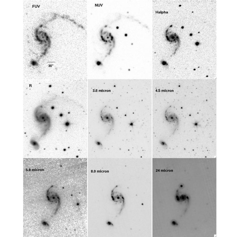
Figure 1: From top (left to right): FUV, NUV, H$\alpha$, R, 3.6 $\mu$m, 4.5 $\mu$m, 5.8 $\mu$m, 8.0 $\mu$m, & 24 $\mu$m. In all the images north is up and east is to the left. The scale bar is 30″ and corresponds to $\sim$8.2 kpc. The large galaxy to the north is NGC 2535 and the smaller companion to the south is NGC 2536.

In Figure 1 we present the FUV, NUV, H$\alpha$, R band, 3.6 $\mu$m, 4.5 $\mu$m, 5.8 $\mu$m, 8.0 $\mu$m, and 24 $\mu$m images of Arp 82 respectively. The bridge and countertail are easily seen in the FUV and NUV images. The tail region is much more prominent in the UV than in the IR as one would expect. The UV traces older stars than H$\alpha$, which is a tracer of massive stars. Since H$\alpha$ correlates with warm dust in emission (Roussel et al., 2001 and references therein), we expect the 8 $\mu$m to be very close to areas harboring photon dominated regions (PDRS) and massive stars.

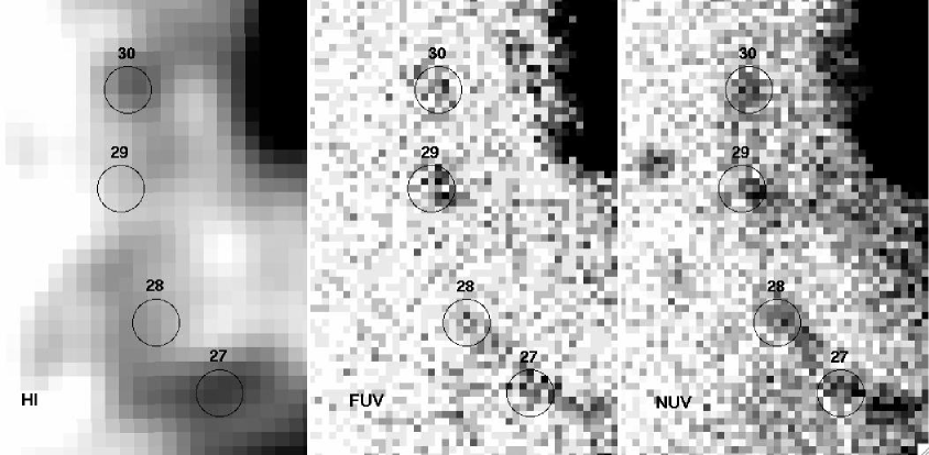
Figure 2: Expanded FUV (top left) and 8.0 $\mu$m (top right) images with the clumps identified. Clumps 27-30 lie along the H I arc and are shown on the FUV image. Zoomed in H I map (Kaufman et al., 1997), FUV, and NUV images of the H I arc (bottom left, middle, and right respectively).

Several bright star forming regions (clumps) can be seen in the 8 $\mu$m image (Figure 2). We have identified 26 clumps by visual inspection of the 8 $\mu$m image. To strengthen our detection criterion, we required the measured fluxes of the clumps to be greater than 3$\sigma$ of the sky background times the square root of the number of pixels in the photometric aperture. All 26 clumps were detected in the FUV, NUV, R band, 8 $\mu$m, and 24 $\mu$m images, 24 were detected at the 3$\sigma$ level in H$\alpha$, 25 were detected at 3.6 $\mu$m, 23 were detected at 4.5 $\mu$m, and 24 were detected at 5.8 $\mu$m.

Clump 13, in the very center of NGC 2535, is clearly visible in the IRAC and MIPS images. It is also visible in the H$\alpha$, R, and NUV images, however, it almost disappears in FUV. This could be the result of reddening. The L(IR)/L(FUV) ratio (see §4.2) is a measure of the total UV opacity. L(IR)/L(FUV) is greatest for knot 13, consistent with a large reddening. The bright clump at the beginning of the northern tail, 21, is among the brightest of the star forming regions in Arp 82 at 8 $\mu$m and 24 $\mu$m. The bright clump at the end of the northern tail, 22, has a significantly higher H$\alpha$/mid-infrared ratio than the other clumps.

Clumps 12, 14, and 15 make up the bright ‘ocular ring’ at the outer edges of the spiral region in NGC 2535. Notice that the ‘ocular ring’ is bright in all the bands. Dramatic ‘beads on a string’ features are visible: chains of evenly-spaced star formation complexes (Figure 1). These clumps are separated by a characteristic distance scale of $\sim$1 kpc, implying that they are caused by gravitational collapse of interstellar gas clouds under self-gravity (Elmegreen & Efremov, 1996).

In addition to the 26 clumps described above, we identified 4 clumps along the H I arc to the southeast by visual inspection of the FUV image. These additional clumps, 27, 28, 29, and 30, can also be seen clearly in H I (Kaufman et al., 1997). See §4.5 for details on these additional clumps, which are discussed separately.

3.2 Background Subtraction

To properly subtract an appropriate sky value from our flux measurements, to minimize contributions from neighboring clumps, to correct for a gradient in the 5.8 $\mu$m image, and to remove the effect of muxbleed in the 8.0 $\mu$m image, we created and subtracted background images. These background images were created by masking the clumps in the original images and replacing them with the median background values. Then the entire background images (including the non clump component of the parent galaxies) were boxcar smoothed. The contamination by the parent galaxies was therefore removed. We determined the replacement values by using the IRAF task IMEXAM with a 50$\times$50 pixel window to measure the median sky values in several regions near the galaxies. The sizes of the replacement window were chosen to be bigger than our photometric apertures and the smoothing windows were chosen to be much larger than the replacement windows. The IRAF task BOXCAR was used to smooth the background images. Finally the smoothed background images were subtracted from the original images. Photometry was performed on the background subtracted images.

3.3 Photometry

The measured fluxes of the clumps are listed in Table 2. The first column is the clump ID, columns 2-3 are the RA and DEC, columns 4-5 are the UV fluxes, columns 6-7 are the optical fluxes, and columns 8-12 are the IR fluxes. The measured colors are listed in Table 3.

The photometry was performed on the FUV and NUV images with the IRAF task PHOT in the DAOPHOT package. We used circular apertures of 3 pixel radii (4$\farcs$5) centered on the positions of the clumps. Using stars in the field, we determined an FUV aperture correction of $\sim$1.15 and an NUV aperture correction of $\sim$1.45, by comparing fluxes in 3 pixel (4$\farcs$5) with those in 25 pixel (37$\farcs$5) apertures. The UV fluxes were converted to magnitudes on the AB system (Oke, 1990).

The H$\alpha$ and R band photometry was performed on the SARA images using 9 pixel (4$\farcs$5) radii apertures. As discussed in §3.2, we subtracted a background image. Calibration was accomplished using the standard stars HZ 14 and Hiltner 600 (Oke, 1974), and correcting the H$\alpha$ flux for [N II] by assuming H$\alpha$/[N II]$\sim$3, typical of H II regions (Osterbrock, 1989). We determined the aperture correction for the SARA H$\alpha$  and R band images by measuring the flux of several stars on the images through 7.5 pixel and 25 pixel apertures. The SARA H$\alpha$ aperture correction is $\sim 1.18$ and the R band aperture correction is $\sim$1.33.

The photometry on all 4 IRAC images was done with 3 pixel (3$\farcs$6) apertures. As with the UV and optical data, no sky annuli were used due to crowding. Instead we created and subtracted a background image as described previously. We used aperture corrections of 1.12 for the 3.6 $\mu$m and 4.5 $\mu$m  bands, 1.14 for the 5.8 $\mu$m band, and 1.23 for the 8.0 $\mu$m band (IRAC Data Handbook v2.0).

The 24 $\mu$m fluxes of the clumps were measured with a 1.22 pixel (3″) aperture. The same technique was used to remove background as described above. According to the MIPS Data Handbook, the aperture correction for a 3″aperture is 3.097.

We measured the flux of the entire Arp 82 system in all our observed wavebands using the IRAF task IMSTAT on rectangular regions covering the full observed extent. The sky background was determined from the mean counts in multiple box regions located around Arp 82, selected to avoid bright stars.

To determine the uncertainties in the flux measurements, we assumed that Poisson noise was the dominant component. To account for the effects of different methods of sky subtraction, we repeated the photometry on the original galaxy images in each band using the mode of a sky annulus of radii 1 pixel larger than the photometric aperture radii and width 5 pixels as our sky subtraction. We took the square root of the difference in counts between the annulus subtracted measurements and the background subtracted measurements as an additional source of uncertainty. This additional uncertainty was added in quadrature to the statistical uncertainties. Typically the additional uncertainties were less than 10%, except in the crowded regions where the additional uncertainties were typically 15%-20%.

4 RESULTS

4.1 Spitzer Colors and Gradients

To study the IR color variations of the clumps with position, we plotted the various IR colors as a function of distance from the NGC 2536 nucleus. Figure 3 plots the [3.6]$-$[4.5] colors as a function of distance from NGC 2536. Open squares represent clumps in NGC 2536, x’s represent clumps in the bridge, stars represent clumps in the spiral and filled squares represent clumps in the countertail. Figure 4 plots the [4.5]$-$[5.8] colors against distance from NGC 2536. Figure 5 shows the [5.8]$-$[8.0] colors as a function of distance from NGC 2536.

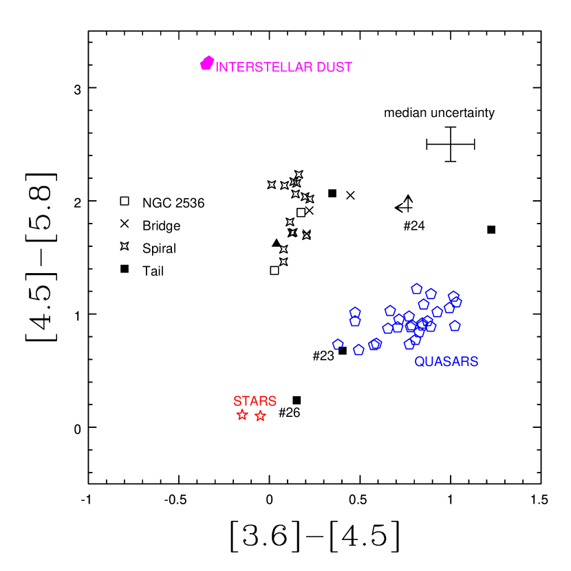
Figure 7: [4.5]-[5.8] vs [3.6]-[4.5]. The symbols are the same as figure 13. Clump 24 is plotted as a lower limit.

Figure 6 plots the [5.8]$-$[8.0] color against the [4.5]$-$[5.8] color. Figure 7 compares the [4.5]$-$[5.8] color with [3.6]$-$[4.5]. Also included in these two figures are the predicted IRAC colors for interstellar dust (Li & Draine, 2001), the Sloan Digitized Sky Survey quasars in the Spitzer Wide-Area Infrared Extragalactic Survey (SWIRE) Elais N1 field (Hatziminaoglou et al., 2005), and the colors of M0 III stars from M. Cohen (2005, private communication) and field stars from Whitney et al. (2004). The quasars have redshifts between 0.5 and 3.65; since their spectral energy distributions are power laws, their infrared colors do not vary much with redshift. From these figures, it can be seen that clumps 23 and 26 have colors consistent with those of quasars and field stars respectively and may not be part of Arp 82.

From Figures 6 and 7, it can be seen that most of the clumps have [3.6]$-$[4.5] colors similar to the colors of stars, (0.0$\pm$0.5 magnitudes) (M. Cohen 2005, private communication; Whitney et al., 2004) implying these bands are mostly dominated by starlight. The [4.5]$-$[5.8] colors are generally very red, except for the two low S/N clumps in the tail, 23 and 26. Most of the clumps have [4.5]$-$[5.8] colors between those of the ISM and stars, indicating contributions from both to this color. Most of the [5.8]$-$[8.0] colors are between $\sim$1.6 and 2, similar to that of the ISM (Li & Draine, 2001). Thus these bands are partially dominated by interstellar matter. Clump 24, which is in the northern tail, has colors similar to those of ISM (upper limits are shown). Thus, this appears to be a very young star formation region with little underlying old stellar population.

Figure 8 plots the ratio L(H$\alpha$)/L(3.6 $\mu$m) against 8.0 $\mu$m magnitude and Figure 9 compares the ratio L(H$\alpha$)/L(8.0 $\mu$m) with 8.0 $\mu$m magnitude. Here and throughout we define L($\lambda$) = $\Delta\lambda$L_λ($\lambda$) and $\Delta\lambda$ is taken as the width of the band (IRAC Data Handbook). The L(H$\alpha$)/L(3.6 $\mu$m) ratio is a proxy of the instantaneous star formation normalized by an effective stellar mass of the knots. Note that there is considerable scatter in both ratios, even in L(H$\alpha$)/L(8.0 $\mu$m), in spite of the fact that both H$\alpha$ and 8 $\mu$m trace star formation. Note that clump 22 (at the end of the northern tidal tail) and clump 21 (at the beginning of the northern tidal tail) have significantly higher H$\alpha$/mid-infrared ratios than the other clumps. Clumps 23 and 26 (in the northern tidal tail region) were below our detection threshold in H$\alpha$.

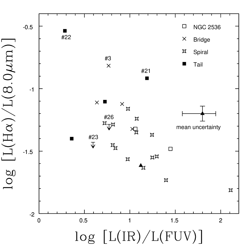
Figure 11: Log[L(H$\alpha$)/L(8.0$\mu$m)] vs Log[L(IR)/L(FUV)]. The symbols are the same as in Figure 8. The mean uncertainty for the horizontal axis reflects only the scatter in the L(IR) calibration.

To test whether the variations in L(H$\alpha$)/L(3.6 $\mu$m) and especially L(H$\alpha$)/ L(8.0 $\mu$m) are due in part to extinction of the H$\alpha$ emission, we plot the ratios against L(IR)/L(FUV) (Figures 10 and 11), where L(IR) is the total infrared luminosity. L(IR)/L(FUV) is a good proxy for extinction (see §4.2). The L(IR), of the clumps was estimated from the measured 8.0 $\mu$m and 24 $\mu$m fluxes using the relation log[L(IR)] = log[$\nu$L(24)] + 0.908 + 0.793 log[L_λ(8.0) / L_λ(24)] (Calzetti et al., 2005). Note that $\nu$L(24) is the monochromatic luminosity with frequency $\nu=1.27\times 10^{13}$ Hz. There is a scatter of $\pm 40\%$ in the L(IR) relation (Calzetti et al., 2005). Weak anti-correlations may be present, especially in the L(H$\alpha$)/L(8.0 $\mu$m) plot, in that the regions with lower dust obscuration tend to have higher L(H$\alpha$)/L(8.0 $\mu$m) ratios. There is, however, a lot of scatter in these plots, suggesting that some of the variations in both the L(H$\alpha$)/L(3.6 $\mu$m) and the L(H$\alpha$)/L(8.0 $\mu$m) ratios are intrinsic. This scatter may be due to PAH excitation by non-ionizing photons contributing to the 8.0 $\mu$m emission.

4.2 Reddening and Ages

The long wavelength IR light is due to the re-processing of UV light, therefore L(IR)/L(FUV) is a measure of FUV opacity or dust optical depth. Calzetti et al. (2000) found that the UV obscuration at 1600 Å is related to the UV opacity by A(0.16$\mu$m)=2.5 log[1/E F(IR)/F(FUV) +1], where E=0.9 is the ratio of the bolometric correction of the UV-to-near-IR stellar light relative to the UV emission at 1600 Å and the dust bolometric correction to the fraction of FIR light detected by the IRAS window. The UV obscuration is related to the extinction by A(0.16$\mu$m)=4.39 E(B$-$V) (Calzetti et al., 2000). Given the above assumptions, the E(B$-$V) of the clumps in Arp 82 range from $\sim$0.3$\pm 0.1$ mag to $\sim$1.2$\pm 0.1$ mag, with a mean of $\sim$0.6$\pm 0.1$. The uncertainties in these E(B$-$V) estimates reflect only the scatter in the L(IR) calibration. Figure 12 is a plot of the log[L(IR)/L(FUV)] versus distance from the NGC 2536 nucleus. It can be seen from Figure 12 that the reddening is generally greater in NGC 2536 and the spiral region, while it is lower in the bridge and tail regions.

We have generated a set of model cluster spectral energy distributions (SED) from the stellar population synthesis model Starburst99 (SB99) code version 5.0 (Leitherer et al., 1999), and convolved these with the GALEX and SARA bandpasses. The SB99 models were generated assuming stellar+nebular continuum emission, instantaneous starbursts, solar metallicity, a Salpeter IMF from 0.1 to 100 $M_{\odot}$, and a total mass of $10^{6}$ $M_{\odot}$. Changes in the evolutionary tracks due to metallicity are small compared to our observational uncertainties, so other abundances were not considered. A second set of models were generated assuming continuous star formation at a rate of 1 $M_{\odot}$ yr^-1. All other assumptions in this second model are the same as the first.

The IRAC images suggest that a significant amount of dust is associated with the clumps. To correct the models for dust obscuration, we reddened them from 0-1.2 mag in 0.1 mag increments assuming the Calzetti, Kinney, & Storchi-Bergmann (1994) starburst reddening law. The assumption of instantaneous or continuous star formation is quite important. Ages determined assuming continuous star formation may be factors of 10 larger than those assuming instantaneous star formation. The bright FUV, 8 $\mu$m, and 24 $\mu$m clump emission suggest a relatively young stellar population, so instantaneous star formation is our working assumption for the clumps. Once the model IMF, abundance, and star formation type is defined, the location of the clumps on a color-color diagram depend only on the age and reddening.

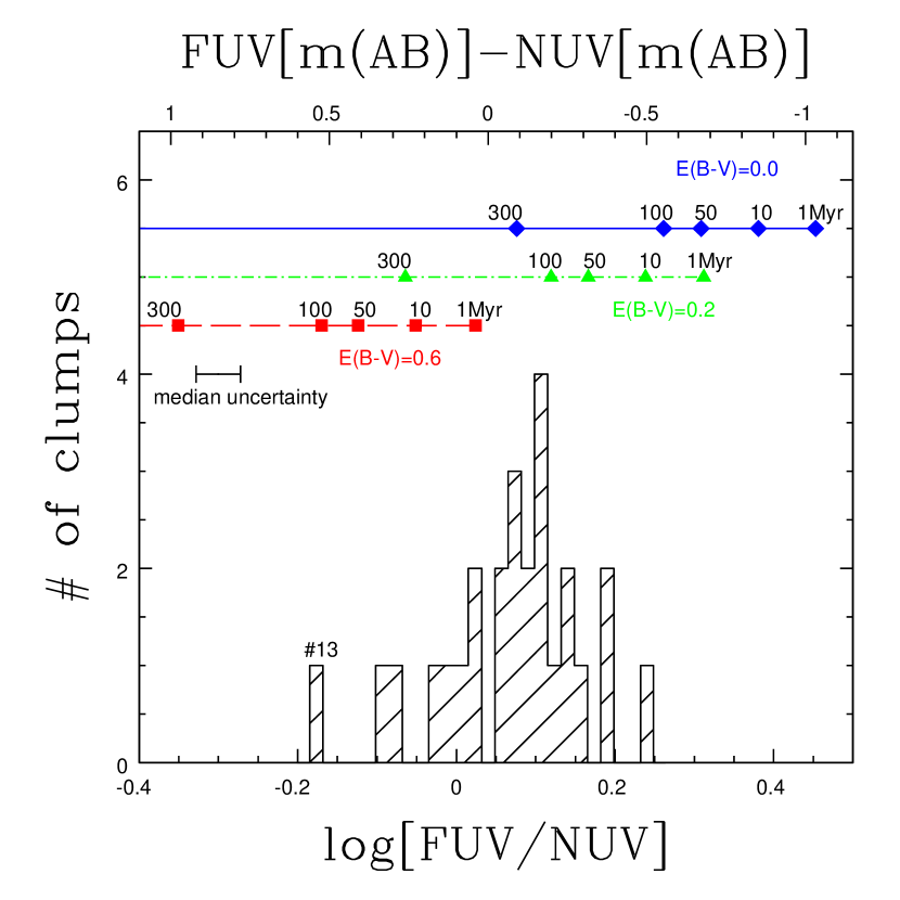
Figure 13: The log(FUV/NUV) distribution of the clumps in Arp 82. At the top are SB99 models with solid line E(B$-$V)=0.0, dot-dash line E(B$-$V)=0.2 and dashed line E(B$-$V)=0.6. SB99 models generated assuming instantaneous star formation, solar abundances, and reddened with the Calzetti, Kinney, & Storchi-Bergmann (1994) reddening law. Ages are marked with diamonds, triangles, and squares. The median uncertainty in flux ratio is also shown. The top axis is in magnitudes.

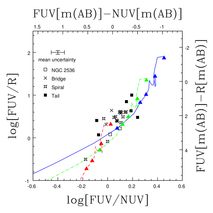
Figure 14: FUV/R vs FUV/NUV. The symbols are the same as in Figure 3. The SB99 models are: solid blue line and filled blue triangles E(B$-$V)=0.0, dot-dashed green line and filled green triangles E(B$-$V)=0.2 and dashed red line and filled red triangles E(B$-$V)=0.6. The SB99 models were generated assuming instantaneous star formation, solar abundances, and reddened with the Calzetti, Kinney, & Storchi-Bergmann (1994) reddening law. The filled triangles plotted along the blue, green, and red curves represent ages of 1, 10, 50, 100, and 300 Myr respectively, with the youngest being at the upper right. The median uncertainty in the clump’s flux ratios is shown. The top and right axes are magnitudes.

Figure 13 is a histogram of the measured FUV/NUV flux ratios of the clumps. The median uncertainty in the ratios is given. At the top of Figure 13 are cluster ages determined from the SB99 code assuming no reddening (blue diamonds), E(B$-$V)$=0.2$ mag (green triangles), and E(B$-$V)$=0.6$ mag (red squares). The age and reddening degeneracy can be seen in this figure. To help break the age/reddening degeneracy we plot a color-color diagram. Figure 14 is a plot of the log(FUV/R) against log(FUV/NUV) with an SB99 model reddened with E(B$-$V)$=0.0$(blue), 0.2(green) and 0.6(red) mag according to the Calzetti, Kinney, & Storchi-Bergmann (1994) reddening law. It can be seen from this figure that the clumps fit nicely between the E(B$-$V)$=0.2$ and E(B$-$V)$=0.6$ models.

To determine the ages and E(B$-$V)s of the individual clumps, we defined the broadband age as the age associated with the log(FUV/NUV) flux and the log(FUV/R) flux of a model point that was closest to the actual data point for each clump in Figure 14. The broadband E(B$-$V) is the reddening applied to the above model. Table 4 lists the broadband ages and extinctions of clumps. We also determined the ages of the clumps from the H$\alpha$ equivalent width (EW(H$\alpha$)) and SB99 (Table 4). The EW(H$\alpha$) traces the ionizing radiation from massive young O stars. These ages will be referred to as EW(H$\alpha$) ages. The EW(H$\alpha$) is in principle a robust probe of clump age, as it is not sensitive to the effects of reddening. However, the EW(H$\alpha$) is sensitive to the determination of the continuum and our assumption about the [N II] emission. The uncertainties in the ages in table 4 reflect only the uncertainties in the measured fluxes. The mean uncertainties on the broadband ages are $+34$ Myr and $-9$ Myr, $\pm 1$ Myr on the EW(H$\alpha$) ages, while the mean uncertainty on E(B$-$V) is $\pm$0.1 mag.

With the exception of the two oldest clumps in the galactic nuclei (clumps 2 and 16), the broadband ages for the Arp 82 clusters range from $\sim$1 to $\sim$30 Myr. Clumps 2 and 16 are considerably older. The cluster ages determined from the EW(H$\alpha$) range from $\sim$6 to $\sim$17 Myr and agree well with the broadband ages. The FUV/NUV and FUV/R trace stars from type B and A and type G and K, respectively; thus they are a better tracer of slightly older clusters than H$\alpha$. The mean broadband E(B$-$V)=0.4 is similar to the mean E(B$-$V) determined from the L(IR) as described previously. From the broadband E(B$-$V) determinations it can be seen that the extinction is generally greatest in the bridge region and the spiral region, consistent with the extinction determined with the far infrared estimate.

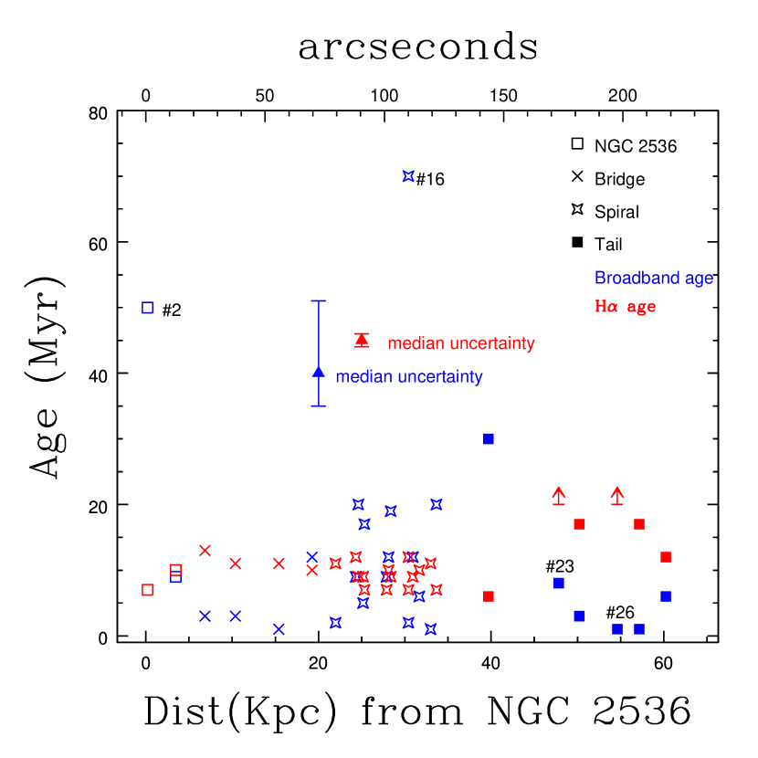
Figure 15: Clump age vs distance from NGC 2536. The symbols are the same as in Figure 3. Blue symbols are the broadband ages and red symbols are the ages determined from EW(H$\alpha$). The uncertainties in ages reflect only the uncertainties in the measured fluxes.

Figure 15 plots the ages of the clumps against distance from NGC 2536. The symbols are the same as before, with the blue symbols being the broadband ages and the red symbols are the EW(H$\alpha$)ages. The mean broadband ages of NGC 2536, the bridge region, the spiral region, and the tail region are 30 Myr, 5 Myr, 15 Myr and 8 Myr respectively. The mean EW(H$\alpha$) ages of NGC 2536, the bridge region, the spiral region, and the tail region are 9 Myr, 11 Myr, 9 Myr, and 13 Myr, respectively. Clumps 23 and 26, which may not be part of Arp 82 (see §4.1), were below our detection threshold in H$\alpha$. From the broadband age analysis it appears that the youngest clumps are generally, but not exclusively, in the bridge and tail regions. Clumps 12, 14, and 15 make up the bright “ocular ring” at the outer edges of the spiral region in NGC 2535. These clumps are among the youngest in the spiral region with broadband ages 17, 2, and 9 Myr respectively, and EW(H$\alpha$) ages of 7 Myr.

4.3 Dust and the SFR

The IR luminosity is the re-emission of absorbed UV photons, so the sum of the UV and IR luminosities is a good proxy for the total UV emission and therefore is proportional to the star formation rate (SFR). In Figure 16, we plot the log[L(IR) + L(FUV)] against UV opacity, log[L(IR) / L(FUV)]. A correlation can be seen. In general, as the dust opacity increases so does the log[L(IR) + L(FUV)]. This correlation indicates that the dust opacity, and therefore the amount of interstellar matter, plays an important role in the SFR. Such a correlation has been seen with several other galaxies (Heckman et al., 1998). Calzetti et al. (2005) find a correlation at the $5\sigma$ level for the clumps in M51. Figure 17 is a plot of the log[L(IR)/L(FUV)] vs log[FUV/NUV]. It has been shown for starburst galaxies that the UV dust opacity correlates with the UV colors (Meurer, Heckman, & Calzetti, 1999). For Arp 82 there is a weak correlation at best in the log[L(IR)/L(FUV)] vs log[FUV/NUV] plot. Several of the clumps in Arp 82 are forming stars in the environments of tidal structures, where the physical processes may be different, and likely more diverse, than in nuclear starbursts.

We have determined the total SFR of the clumps using three calibrations. First, we used the relation, SFR($M_{\odot}$ yr^-1)$=4.5\times 10^{-44}$L(IR)(erg s^-1) (Kennicutt, 1998), using L(IR) bootstrapped from the 8.0 $\mu$m and 24 $\mu$m luminosities (§4.1). The clumps have a total SFR_IR of $\sim$2.0$\pm 0.8$ $M_{\odot}$ yr^-1. The uncertainty reflects the scatter in the L(IR) calibration. Second, for comparison, we used the relation SFR($M_{\odot}$ yr^-1)$=1.4\times 10^{-28}$L_ν(FUV)(erg s^-1 Hz^-1) (Kennicutt, 1998). The total SFR_UV of the clumps is $\sim$0.6$\pm 0.1$ $M_{\odot}$ yr^-1, slightly lower than the SFR_IR. Third, also for comparison, we used the relation SFR($M_{\odot}$ yr^-1)$=7.9\times 10^{-42}$L(H$\alpha$)(erg s^-1) (Kennicutt, 1998). The total SFR_Hα of the clumps is $\sim$1.3$\pm 0.2$ $M_{\odot}$ yr^-1, slightly larger than the UV determination and consistent with the SFR_IR. The uncertainties in the SFR_UV and SFR_Hα reflect only the uncertainties in the measured fluxes. No reddening correction has been applied to the L_ν(FUV) or L(H$\alpha$). The SFR_IR is probably the most reliable because it is not nearly as sensitive to extinction effects. However, the IR may include dust heating by non OB stars, even in the clumps, and may overestimate the SFR. Calzetti et al. (2005) find that L(IR) is not directly proportional to extinction corrected Paschen-$\alpha$ in the M51 clumps. The SFR_IR is also sensitive to the L(IR) calibration discussed above. The SFR_IR of the entire Arp 82 system is $4.9\pm 2.0$ $M_{\odot}$ yr^-1, vs $2.4\pm 0.4$ for SFR_Hα. The total clump SFR_IR accounts for about 40% of the entire system SFR_IR.

Figure 18 plots the log[L(IR)+L(FUV)] of the clumps against the distance from the NGC 2536 nucleus. From this figure it can be seen that the SFR is greatest in the spiral region of NGC 2535 and in NGC 2536, with much less star formation in the bridge and tail regions. The lower SFR of the clumps away from the central regions could be due to the fact that less gas was dragged there as a result of the interaction. Less gas spread over a still large volume implies lower densities, lower compressions, and larger clump masses to pull together gravitationally. Also, more turbulence in the tidal structures may require larger masses for the self gravity to overcome the turbulent pressure.

4.4 Masses of the Clumps

From the measured R band fluxes and the ages and extinctions implied by the broadband colors, we have determined masses for each of the clumps in Arp 82 using our SB99 models. These masses of the clumps are given in Table 5. The first column is the clump ID. The second column is the region the clumps can be found in and the third column is the mass determined by this method (mass_R). For comparison, in Table 5 we also provide the masses of the clumps using the FUV flux (column 4). The masses include stars from 0.1 to 100 $M_{\odot}$. The uncertainties in the clump masses reflect only the uncertainties in the measured fluxes. It can be seen from the large uncertainties that the FUV band is not a reliable mass tracer, as one would expect. The R band is a more reliable tracer of mass than the FUV band because the more populous lower mass stars contribute more to the R band flux.

The more massive clumps tend to be found in the spiral region while the least massive clumps are in the tidal features. The clumps have a median mass_R of about $8\times 10^{7}$ $M_{\odot}$. The ten tidal clumps make up only about 3% of the total clump mass_R. The 2 clumps in the small companion, NGC 2536, and the 2 largest clumps in the nucleus of NGC 2535 (13 and 16) make up about 82% of the clump mass_R.

As a test of the validity of our mass_R determinations, we plot the 3.6 $\mu$m luminosity against mass_R (Figure 19). A strong correlation is seen in this figure. In Figure 14, it was shown that the 3.6 $\mu$m band is dominated by stars, so clump fluxes in this band are a good proxy for mass.

We determined the mean mass to light ratios of the clumps, $\alpha$=(M/M_⊙)/(L/L_⊙), using the mass_R and the R band luminosities. We determined L/L_⊙ by assuming a solar absolute R magnitude of 4.46 (Bell & de Jong, 2001). We find that the mean clump mass to light ratio is $\alpha=0.77$ and the median $\alpha=0.61$. The clump mass to light ratios are plotted against distance from NGC 2536 in Figure 20.

4.5 H I Arc

An interesting tidal feature is clearly visible in the southeast of the FUV image (Figure 2). This ‘arc’ is also visible in the H I maps of Kaufman et al. (1997) and was not detected in their optical B and I images. Kaufman et al. (1997) concluded that this feature was a gaseous structure and suggest that it is a wake in the gas produced by the passage of the companion within or close to the extended H I envelope. Its clear presence in the UV images shows it does have a stellar component with fairly young stars. Other UV-bright tidal features that are optically faint and coincident with H I density enhancements have been observed with GALEX (see for example, Neff et al., 2005). A previously undetected tidal feature in NGC 4435/8 was discovered by Boselli et al. (2005) with GALEX.

In addition to the 26 clumps discussed above, we identified 4 clumps in this H I arc. These clumps are numbered 27, 28, 29 and 30 (Figure 2). The clumps were identified visually on the FUV image. We imposed the same detection criterion as described above. All 4 clumps were detected in the FUV and NUV. Clumps 27, 28, and 30 were detected in H$\alpha$, clumps 27 and 30 were detected in R band and 8.0 $\mu$m, while only 30 was detected in 24 $\mu$m. None of the H I arc clumps were detected in 3.6 $\mu$m, 4.5 $\mu$m, or 5.8 $\mu$m.

The H I column densities for the clumps in this arc range from $6\times 10^{20}-1\times 10^{21}$ cm^-2 (Kaufman et al., 1997). By comparing the FUV/NUV and FUV/R colors of the H I arc clumps 27 and 30 to SB99 we find that they have broadband ages of $7^{+83}_{-0}$ and $6^{+74}_{-3}$ Myr respectively and E(B$-$V)$=0.1^{+0.0}_{-0.1}$ and $0.2^{+0.1}_{-0.2}$ mag respectively. This very low extinction is consistent with the apparent lack of dust suggested by the low IR fluxes. Clumps 27 and 30 have a mass_R of $0.32^{+4.24}_{-0.10}\times 10^{6}$ $M_{\odot}$ and $0.52^{+6.95}_{-0.30}\times 10^{6}$ $M_{\odot}$ respectively.

4.6 The Underlying Stellar Population

In sections 3 and 4, we have extensively discussed the young star-forming clumps in Arp 82. To investigate the underlying stellar population, we subtracted the total clump flux from the total flux in each waveband. We estimated the age and extinction of this underlying population by comparison to a set of SB99 models similar to that described in §4.2. Because an older population could not be effectively modeled with the assumption of an instantaneous burst, we instead generated a model assuming a continuous SFR of 1 $M_{\odot}$ yr^-1. All other model assumptions were the same as before. From the FUV/NUV and FUV/R ratios and SB99 we found that the underlying population was best matched to a model with E(B$-$V)$=0.3$ mag and an age of $\sim 2$ Gyr. The E(B$-$V) estimated here is similar to the extinction we determined for the clumps.

This suggests that the underlying diffuse stellar component in Arp 82 is dominated by a $\sim 2$ Gyr population and that the progenitors may have been of very late type or low surface brightness galaxies with very modest underlying old stellar populations. It should be noted that the FUV/NUV and FUV/R ratios are more sensitive to young and intermediate age stars than truly old stars. It is possible there is an older underlying population in Arp 82 that we are not able to detect. Without the aid of near-IR bands that reflect the peak contributions from M stars, we cannot rule out the presence of a truly old, $\sim$10 Gyr, population. Future work with proposed near-IR maps and optical spectra will further constrain the age of the underlying population.

5 COMPARISON WITH A NUMERICAL SPH MODEL OF THE INTERACTION

The distinctive morphology of this system provides strong constraints on any numerical model of the interaction. Arp 82 is an M51-type system with a strong bridge as observed in the optical/IR bands and in the 21 cm radio band, and a long countertail stretching to the northwest. These features, together with the ocular waveform (Elmegreen, Kaufman, & Thomasson, 1993; Kaufman et al., 1997) in the primary disk suggest that the encounter is strongly prograde for the primary galaxy. That is, the companion orbits the primary in the same sense as the primary rotates, and the companion orbital plane is close to the primary disk plane. These features also constrain interaction time scales. On one hand, an ocular wave is a relatively short-lived feature, though it also takes some time to develop (see e.g., the models of the NGC 2207/IC 2163 system of Struck et al., 2005). On the other hand, the length of the primary tail suggests that this interaction has been underway for some time. This is affirmed by the H I observations (Kaufman et al., 1997), which indicate that not only has there been time to form the bridge, but also time to transfer significant amounts of gas through the bridge to the companion. Finally, the mix of young and intermediate age populations yielded by the population synthesis modeling suggests that the interaction has been underway for a time comparable to the age of the intermediate age populations.

At the same time, the observed FUV/NUV and FUV/R ratios suggest that the star formation in the tail and the bridge, is recent. The clumps in the tail are among the youngest with ages of less than 70 Myr, and perhaps as young as a few Myr. This is much less than the likely kinematic time scale for the arm to reach its current distance from the center. The companion is very disturbed, both morphologically and kinematically, so we cannot derive much information about the interaction from its structure. However, we would expect a successful model to reproduce its disturbed structure, and intense star formation activity.

The H I mapping of Kaufman et al. (1997) provides a good deal of kinematic information on this system. However, for present purposes we seek an approximate model that can help understand the range of time scales indicated by large-scale morphological structures and the general star formation history. We have not attempted to produce a model that is sufficiently detailed to match the kinematics as well.

5.1 Model Details

The model described below was produced with the SPH code of Struck (1997, also see Struck et al. 2005). This code employs some simplifications to allow it to efficiently explore a range of collision parameters. The foremost of these is that rigid dark halo potentials are used, and hydrodynamic forces are computed on a grid with fixed spacing. Local gravitational forces are computed between particles in adjacent cells, to capture local gravitational instabilities, which are important for modeling star formation. In addition to the halos the model galaxies have disks consisting of gas particles and collisionless star particles of equal mass.

In the models described below the following particle numbers were used: 42900 primary disk gas particles, 5640 primary star particles, 13590 companion disk gas particles, and 2490 companion star particles. The extensive gas disks, and limited stellar disks, used in these models represent our belief that the progenitor galaxies were likely of very late type or were low surface brightness galaxies, with very modest old stellar populations.

We adopt the following scaling constants for the model: time unit $=400$ Myr, length unit $=2.0$ kpc, and mass unit $M_{h}=3.9\times 10^{10}M_{\odot}$. With these scalings we obtain a peak rotation velocity of about 200 km s^-1 in the primary, which reasonably matches the uncertain observational constraints (Kaufman et al., 1997).

The mass ratio of the two galaxies can be estimated by comparing the mass of each within a radius of 20 kpc; it is 0.13 (Kaufman et al., 1997). The form of the rigid potential used gives a test particle acceleration of,

$$a=\frac{G{M_{h}}}{{\epsilon}^{2}}\ \frac{r/{\epsilon}}{(1+r^{2}/{\epsilon}^{2})^{n_{h}}},$$

where $M_{h}$ is a halo mass scale, $\epsilon$ is a core radius (set to 2.0 and 4.0 kpc for the primary and companion, respectively), and the index $n_{h}$ specifies the compactness of the halo. For the primary we use $n_{h}=1.1$, which gives a slightly declining rotation curve at large radii. For the companion we take $n_{h}=1.35$, which gives a declining rotation curve at large radii. We have not undertaken a detailed examination of the effects of different values for these exponents. Because the two galaxies have different halo potentials, the effective mass ratio (i.e., the ratio of masses contained within radii equal to the galaxy separation) is large for small separations, and small for large separations. This effect makes encounters between the two galaxies quite impulsive. The model presented here includes the effects of dynamical friction with a Chandrasekhar-like frictional term (Struck & Smith, 2003). The effects of this term are small except for brief times near closest approach. It ultimately draws the two galaxies into a merger at times shortly past the present (the second close encounter).

The initial disk sizes of the primary gas disk was 19.2 kpc, and the companion gas disk was 14.4 kpc. These values, and the initial orientation of the companion, are fairly arbitrary; we have not attempted to optimally fit them. The primary disk was initialized in the computational x-y plane. The companion disk was initialized in the x-y plane and then tilted $20^{\circ}$ around the y-axis such that positive x values had positive z values. It was then tilted $-25^{\circ}$ in the x-y plane around the y-axis. After the run the whole model x-y was rotated by $-90^{\circ}$ in the x-y plane around the primary center to better fit the observed orientation. The initial position and velocity vectors of the companion relative to the primary center were: (0.0 kpc, 30.0 kpc, 4.0 kpc) and (200 km s^-1, -60 km s^-1, -25 km s^-1).

5.2 Model Results

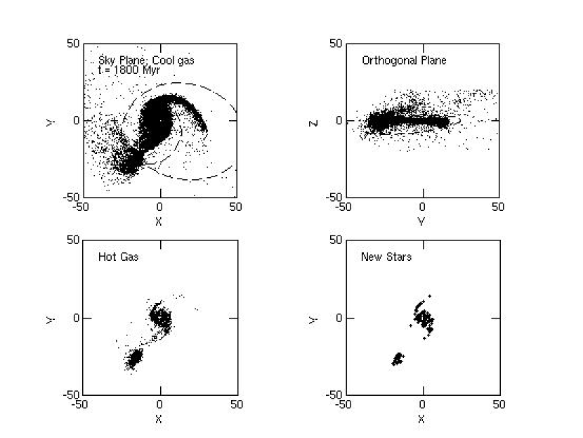
Figure 21: Snapshots of the model at a time near the present. The upper panels show two orthogonal views of the gas particles. The primary’s position is fixed at the origin. The dashed curve also shows the orbit of the companion center relative to the primary, starting from the point marked by a cross, and continuing through the present to the future merger. The coordinate values are given in kpc with the adopted scaling. The lower panels show gas particles that have either just turned on star formation feedback (lower right), or have recently turned on feedback, and so heated the gas (lower left). The latter thus gives a cumulative picture of recent star formation, rather than just the immediate star formation.

Figure 21 shows various views of the model results at a time near the present, as judged by the morphology. All axis labels are in kpc with the adopted model scaling. The top two panels show the relative orbit of the companion as a dashed curve from the beginning of the run and into the future, with the cross marking the initial position. The top two panels also show the distribution of cold (or unheated) gas particles from the two disks at the present time. The bottom right panel shows gas particles in which the threshold density has been exceeded, so star formation and heating have been turned on in them. The lower left panel shows the distribution of hot gas particles, i.e., particles in which star formation heating was on recently, but which have not had time to cool. The initial position and about the first three fourths of the trajectory are not strongly constrained by observation, and are fairly uncertain.

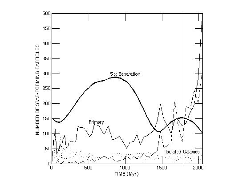
Figure 22: Shows star formation histories of the model galaxies. Specifically, the thin solid curve shows the number of star forming particles within 24 kpc of the center of the primary galaxy as a function of time. The dashed curve shows the number of star forming particles within 12 kpc of the center of the companion galaxy as a function of time, and the dotted curves show the corresponding quantities for the two galaxies in isolation. The values of the integration radii were chosen to enclose the whole disk of the individual galaxies, without including particles from the other galaxy. The bold solid curve shows the separation between the galaxy centers in kpc as a function of time, multiplied by a factor of 5 in order to use the same y-axis scale. Comparison of this curve to the thin solid and dashed curves allows one to see how the SFR depends on separation. The vertical line denotes the approximate present time.

The two initial gas disks were very similar, so the contrast at the present time is quite striking. The most prominent tidal features, the bridge and tail of the primary, were largely formed as a result of the most recent close encounter. This encounter occurred at a position angle of about $45^{\circ}$ in Fig. 21. The bold curve in Figure 22 shows the separation distance. At the present time the two galaxies have moved somewhat apart after close approach. The upper left panel of Figure 21 suggests that after this time the two will merge.

Figure 21 shows that this model does a pretty good job of reproducing the extensive gas bridge observed in this system (also see the earlier model of Klaric, 1993 and Kaufman et al., 1997), and the long, fairly narrow tidal tail. The optical tail is unusually long, about three times the size of the primary disk. The model tail is only about two times the size of the star-forming part of the primary disk, which may indicate that the initial model gas disk should have been larger.

There was an earlier close encounter near the beginning of the run. The primary also formed a bridge and tail after this encounter. However, these features were weaker, and did not persist or leave much sign of their existence in the current morphology.

This is not true in the case of the companion. The initial encounter was close enough and the orientation of the companion was such that a strong radial (ring-like) wave was generated. This, and subsequent tidal forces, resulted in much of the outer gas disk of the companion being pulled off in a long and very diffuse plume. Initially, the gas retained by the companion expanded outward in the ring wave, but most of it fell back in close to the time of the most recent close encounter. The two effects combined to put a large mass of compressed gas in the core of the companion and trigger repetitive starbursts (Fig. 22).

We have attempted to reproduce a plausible star formation history of both galaxies with the models. The results are shown in Figure 22. First of all, the disk structure, gas particle mass (about $1.3\times 10^{5}M_{\odot}$), and the star formation threshold density were all initialized such that the two gas disks would have a low rate of star formation in isolation. The dotted curves in Fig. 22 show the star formation history of the two disks run in isolation for a time of slightly more than 2 Gyr. After some initial transients both disks settle to a very low rate of stochastic star formation. In the interaction simulation, the companion retains a low rate of star formation up to the time of the most recent close encounter. As a result of the tidal distortion and the repetitive starbursts the companion could be converted from a very regular low-surface-brightness disk to the compact, but irregular form observed now.

The interaction is prograde for the primary galaxy, so even the weak initial encounter triggers an enhanced rate of star formation in the core of the primary, and somewhat later in induced spiral waves. Nonetheless, even this enhanced rate is modest until the most recent encounter, when a burst is triggered with about 10 times the SFR of the isolated primary. The model further predicts that with merger in the near future the SFR will rise precipitously. This prediction cannot be checked, of course, but it is in accord with what we know about gas-rich, infrared luminous, merging systems.

Nonetheless, this range of SFR amplitudes in the model is probably not enough to account for the observation that the bulk of the star formation (SF) has occurred in the last $\sim 2$ Gyr. Given the long time before the interaction, even at the low quiescent rates shown in Fig. 22, only of order 5% of the stars would be produced in the interaction with the rates shown there. It is likely that the true quiescent SFRs were even lower, and the core burst rates in the first interaction were much higher than in the model of Fig. 22. The former could be easily achieved by modifying the threshold density parameter for SF feedback. Modeling stronger bursts would probably require higher particle resolution, a more massive companion (to increase the perturbation on the primary) and more sophisticated thermal physics. Clearly, this system poses interesting tests for phenomenological feedback models, though we believe more detailed modeling should await spectral observations that provide stronger constraints on the stellar population ages.

We note for completeness that if the model were run backwards from its rather arbitrary initial conditions, it would have spent at least another Gyr in an outward loop. This assumes that the adopted halo potentials extend that far out, and that the loop is like the one illustrated in Figs. 21 and 22, but somewhat larger due to the modest effects of dynamical friction. It is equally likely that the halo potentials start to fall off more rapidly at large separations, and that the companion took a much longer time to come in from a much greater separation. Then the initial encounter modeled here would have been the first.

Finally, it is interesting to use Fig. 22 to compare the SFR to the galaxy separation over the course of the simulation. Generally, these two quantities correlate, but not monotonically. This is illustrated by the echo bursts that occur near the present time, and well after the last close encounter.

6 COMPARISON TO OTHER GALAXIES

How do the star forming properties of the Arp 82 clumps compare to other galaxies studied in detail by Spitzer? The [4.5]$-$[5.8] and [5.8]$-$[8.0] colors of the Arp 82 clumps are typically redder than those in Arp 107, the other SB&T galaxy we have studied in detail (Smith et al., 2005). This indicates younger stellar populations on average in Arp 82; consistent with its more quiescent IRAS properties. The IRAC colors of the clumps in Arp 82 are generally similar to those in IC 2163 and NGC 2207 (Elmegreen et al., 2006). The log[FUV/NUV] distribution of the clumps in Arp 82 resembles that of the clumps in M51 (Calzetti et al., 2005). This suggests that the clump ages in the two systems are likely similar.

Very young star forming regions have also been found in a myriad of other interacting galaxies using UV and optical studies. For example, Weistrop et al. (2004) find that 59% of the star forming regions in the advanced merger NGC 4194 are younger than 10 Myr, while Hancock et al. (2006) report that 14 star forming regions in NGC 4194 are $\sim$6 Myr. Hancock et al. (2003) find that several knots in NGC 3395 and NGC 3396 have ages less than 20 Myr; some are as young as 5 Myr. Eggers et al. (2005) reports that the ages of 12 knots in NGC 3994 are less than 20 Myr and the ages of 22 knots in NGC 3995 are younger than 10 Myr. In a study of NGC 1741, Johnson et al. (1999) found star forming regions as young as a few Myr. Johnson et al. (2000) report ages less than 10 Myr for nearly half the knots in He 2-10. The Antennae (NGC 4038/39) has clusters with ages ranging from $\sim$5-10 Myr (Whitmore, 2003).

Most of the star forming regions discussed in the above galaxies are proto-globular cluster candidates. Some of the clumps in Arp 82 are similar in age to these star forming regions, but with the exception of a few clumps in the tail, are typically too massive to be proto-globular clusters. The mean mass_R of the Arp 82 clumps is $3.6\times 10^{8}$ $M_{\odot}$, much more massive than typical Galactic globular clusters, which have masses $\sim$10${}^{5}-10^{6}$ $M_{\odot}$ (Pryor & Meylan, 1993). The mass of 15 clumps in IC 2163 and NGC 2207 were found to range from $2\times 10^{4}$ to $1\times 10^{6}$ $M_{\odot}$ (Elmegreen et al., 2006). Calzetti et al. (2005) find that the brightest H$\alpha$ knot in M51 is $\sim$2$\times 10^{5}$ $M_{\odot}$, while the UV emitting sources range in mass from $\sim$6$-$8$\times 10^{7}$ $M_{\odot}$. The Tidal Dwarf Galaxies (TDG) in the Braine et al. (2001) sample have masses ranging from $2\times 10^{6}$ $M_{\odot}$ to $4.5\times 10^{8}$ $M_{\odot}$, while the TDG candidates in the Higdon, Higdon & Marshall (2006) sample have masses $\sim$2$\times 10^{7}$ $M_{\odot}$ to $\sim$3$\times 10^{8}$ $M_{\odot}$, similar to the masses of most of the clumps in Arp 82. However, clumps 22, 24, and 25 (in the Arp 82 tail) have masses of $2^{+22}_{-1}-10^{+27}_{-5}\times 10^{6}$ $M_{\odot}$ which are similar to that of Galactic globular clusters and the UV sources in M51.

The star forming clumps in Arp 82 are larger than globular clusters. The mean full width at half maximum of the clumps in R band is $\sim$1 kpc. This size is much larger than typical Galactic globular clusters which have effective radii of about 3 pc (Miller et al., 1997). The clumps have sizes and masses more like giant star forming complexes and TDGs than globular clusters. Given the limited resolution of these data, it is possible that some of the clumps are comprised of multiple unresolved clusters. Elmegreen et al. (2006) found that the Spitzer clumps in the IC 2163 ocular, which are similar to ours, were resolved into smaller clusters by HST.

For a sample of Galactic globular clusters, Pryor & Meylan (1993) find mass to visible light ratios that range from 0.5 to 6.2 with a mean ratio of $\sim$2.4. Although the mean mass to light ratio we derive for the clumps is within this range, it is far below the Pryor & Meylan (1993) mean. Figure 20 is a plot of the mass to light ratios of the clumps against distance from NGC 2536.

The SFR_IR of the entire Arp 82 system is $4.9\pm 2.0$ $M_{\odot}$ yr^-1. The SFR alone may not adequately suggest an enhancement in star formation. The [3.6]$-$[24] color is a good measure of the ratio of the SFR to the total stellar mass. The total system [3.6]$-$[24] color of Arp 82 is 5.9, near the peak of the Arp disk distribution and redder than the majority of the normal spirals in the Spitzer infrared nearby galaxy sample (SINGS) (see Smith et al., 2006), suggesting an interaction-induced enhancement in star formation.

7 SUMMARY

We present a UV, optical, and mid-IR study of the star forming properties of the interacting pair Arp 82, using data from GALEX, SARA, and Spitzer. We have identified 30 star forming regions (clumps). The clumps contribute 33% and 40% of the total FUV and NUV emission respectively and similar percentages (26%, 26%, 28%, 33% and 36%) of the R band and IRAC bands (3.6, 4.5, 5.8, and 8.0 $\mu$m respectively). Larger percentages are found at 24 $\mu$m and H$\alpha$ (70% and 55%, respectively). The relatively low clump contribution to the 8.0 $\mu$m emission implies a considerable contribution to the non-clump 8.0 $\mu$m from PAH heating by non-ionizing stars.

The clumps have [3.6]$-$[4.5] colors similar to the colors of stars. Most of the clumps have [4.5]$-$[5.8] colors between those of the ISM and stars, indicating contributions from both to this color. Most of the [5.8]$-$[8.0] colors are similar to that of the ISM. Thus these bands are dominated by interstellar matter. Clumps 23 and 26 have colors consistent with those of quasars and field stars respectively and may not be part of Arp 82. There is considerable scatter in both the L(H$\alpha$)/L(3.6 $\mu$m) and L(H$\alpha$)/L(8.0 $\mu$m) ratios of the clumps. Some of the variation in the L(H$\alpha$)/L(8.0 $\mu$m) ratios maybe due to extinction, but some is intrinsic, perhaps due to polycyclic aromatic hydrocarbon (PAH) excitation by non-ionizing photons.

The broadband ages of the clumps indicate that the majority are less than 100 Myr and could be as young as a few Myr. The clumps in the tidal features tend to be younger. The extinction across the galaxy varies from E(B$-$V)$\sim$0.2${}^{+0.1}_{-0.2}-0.7^{+0.2}_{-0.0}$ mag, being generally greater in NGC 2536 and the spiral region and lower in the bridge and tail regions. The masses of these clumps range from a few $10^{6}$ to a few $10^{9}$ $M_{\odot}$, with the two nuclei being by far the most massive, making up 82% of the total clump mass. The total SFR_IR of Arp 82 is 4.9$\pm 2.0$ $M_{\odot}$ yr^-1, with $\sim$16% of the new stars forming in the two nuclei.

We have used an SPH code to model the interaction and reproduce the star formation history. The model indicates that the galaxies have undergone two close encounters. In the model, the primary suffered a mild starburst during the first close encounter and a stronger burst more recently, consistent with the observations. In the interaction simulation, the companion retains a low rate of star formation up to the time of the most recent close encounter. The companion may have converted from a very regular low-surface-brightness disk to the compact irregular form observed now, as a result of the tidal distortion and the repetitive starbursts. The model predicts that with merger in the near future the SFR will rise precipitously. This prediction cannot be checked, of course, but it is in accord with what we know about gas-rich, infrared luminous, merging systems.

The star formation history for this system derived from observations and models, suggest that this is a very unusual system. The initial formation of these two galaxies seems to have been as unspectacular as the model star formation transients of the isolated disks shown in Fig. 22. This quiescent initial formation was evidently followed by a long period, only a little less the age of the universe, when very few additional stars were produced. In this sense, galaxy formation got stuck, before normal, late-type disks could be formed. The present interaction and eventual merger may result in an early to intermediate Hubble type disk galaxy.

Since the galaxies in this system are of intermediate mass, their evolution is in rough accord with the downsizing concept, wherein large galaxies are supposed to have formed at early times in dense environments, and most of the current star formation is occurring in much smaller galaxies (see e.g., Juneau et al., 2005; Bundy et al., 2005; Mateus et al., 2006 and refs. therein). Recent work further suggests that most of the stars in intermediate mass galaxies formed 4-8 Gyr ago, and most current star formation is occurring in still smaller galaxies (Hammer et al., 2005 and refs. therein). Arp 82 may be a downsizing outlier, and could provide a local view of the “age of intermediate mass galaxies.” The stellar populations in this relatively nearby system could be studied in much greater detail than those of its higher redshift kin.

Figure 3: [3.6]$-$[4.5] gradient. Open squares represent clumps in NGC 2536, x’s represent clumps in the bridge, stars represent clumps in the spiral and filled squares represent clumps in the counter tail. Clumps 3 and 24 are plotted as upper limits. The mean [3.6]$-$[4.5] color for Whitney et al. (2004) field stars is -0.05, while the predicted value for interstellar dust is -0.35 (Li & Draine, 2001).

Figure 4: [4.5]$-$[5.8] gradient. The symbols are the same as in Figure 3. Clump 24 is plotted as a lower limit. The mean [4.5]$-$[5.8] color for Whitney et al. (2004) field stars is 0.1, while the predicted value for interstellar dust is 3.2 (Li & Draine, 2001).

Figure 5: [5.8]$-$[8.0] gradient. The symbols are the same as in Figure 3. Clumps 3 and 25 are plotted as lower limits. The mean [5.8]$-$[8.0] color for Whitney et al. (2004) field stars is 0.05, while the predicted value for interstellar dust is 2.1 (Li & Draine, 2001).

Figure 6: [5.8]$-$[8.0] vs [4.5]$-$[5.8]. The symbols are the same as in Figure 3. The solid black triangle represents the entire Arp 82 system. The solid pentagons represent predicted IRAC colors for interstellar dust (Li & Draine, 2001), open pentagons represent the Hatziminaoglou et al. (2005) colors of quasars, and the open 5 point stars represent the mean colors of M0 III stars from M. Cohen (2005, private communication) and field stars from Whitney et al. (2004). The median uncertainty is also shown. Clump 24 is plotted as a lower limit.

Figure 8: Log[L(H$\alpha$)/L(3.6$\mu$m)] vs 8.0$\mu$m mag. The symbols are the same as in Figure 3. The solid black triangle represents entire Arp 82 system.

Figure 9: Log[L(H$\alpha$)/L(8.0$\mu$m)] vs 8.0$\mu$m mag. The symbols are the same as in Figure 8.

Figure 10: Log[L(H$\alpha$)/L(3.6$\mu$m)] vs Log[L(IR)/L(FUV)]. The symbols are the same as in Figure 8. The mean uncertainty for the horizontal axis reflects only the scatter in the L(IR) calibration.

Figure 12: Log[L(IR)/L(FUV)] gradient. The symbols are the same as in Figure 3. The mean uncertainty for the vertical axis reflects only the scatter in the L(IR) calibration.

Figure 16: log[L(IR)+L(FUV)] vs log[L(IR)/L(FUV)]. The symbols are the same as in Figure 8. The mean uncertainty reflects only the scatter in the L(IR) calibration.

Figure 17: log[L(IR)/L(FUV)] vs log[FUV/NUV]. The symbols are the same as in Figure 8. The mean uncertainty for the vertical axis reflects only the scatter in the L(IR) calibration.

Figure 18: log[L(IR)+L(FUV)] vs distance from NGC 2536. The L(IR)+L(FUV) is a good proxy for the star formation rate. The mean uncertainty reflects only the scatter in the L(IR) calibration.

Figure 19: Mass_R vs L(3.6$\mu$m). The mass is determined from SB99 and measured R band flux, see text. The symbols are the same as in Figure 3.

Figure 20: Mass to light ratio vs distance from NGC 2536. The symbols are the same as in Figure 3.

Table 1: Observation Log

ID	Telescope	$\lambda_{central}$	Range	Exposure	Date
		($\mu$m)	($\mu$m)	($\#\times$ sec)	(UT)
21197	GALEX	0.153	0.135-0.175	$1\times 1684$	2005-02-24
21197	GALEX	0.231	0.175-0.280	$1\times 3019$	2005-02-13
3247	Spitzer	3.6	3.0-4.2	$6\times 12$	2004-11-01
3247	Spitzer	4.5	3.7-5.3	$6\times 12$	2004-11-01
3247	Spitzer	5.8	4.6-6.9	$6\times 12$	2004-11-01
3247	Spitzer	8.0	5.6-10.3	$6\times 12$	2004-11-01
3247	Spitzer	24	18.0-32.2	$32\times 10$	2005-04-02
- - -	SARA	0.664	0.655-0.675	$16\times 600$	2005-01-03
- - -	SARA	0.694	0.580-0.790	$5\times 600$	2005-01-05

Table 2: Clump Fluxes

Clump	RA	DEC	FUV1	NUV1	H$\alpha^{1}$	R1	3.62	4.52	5.82	8.02	242
	(8:11)	(+25)					$\mu$m	$\mu$m	$\mu$m	$\mu$m	$\mu$m
1	15.061	10:41.75	2.43	2.32	1.58	2.02	0.31	0.23	0.86	2.75	4.94
2	15.930	10:46.47	21.10	16.82	8.55	12.74	2.45	1.61	3.69	10.27	14.74
3	14.452	11:00.64	0.44	0.45	0.25	0.22	0.01	$\leq$0.01	$\leq$0.03	0.09	0.27
4	13.931	11:12.44	1.63	1.51	0.68	0.37	0.05	0.04	0.19	0.52	1.13
5	12.887	11:24.24	3.76	2.97	0.93	1.00	0.09	0.07	0.22	0.69	0.99
6	12.453	11:38.40	2.87	2.41	1.09	1.16	0.14	0.11	0.42	1.31	1.76
7	11.757	11:54.93	2.80	2.19	0.50	1.23	0.10	0.07	0.23	0.80	0.92
8	14.061	12:02.60	4.40	3.45	0.87	1.07	0.13	0.10	0.30	0.94	1.65
9	12.627	12:06.73	3.34	3.59	1.54	1.18	0.14	0.11	0.44	1.28	2.37
10	13.757	12:11.45	8.75	7.56	2.08	2.81	0.36	0.26	0.81	2.30	4.17
11	11.931	12:13.81	5.54	4.63	1.39	2.26	0.37	0.24	1.11	3.42	4.16
12	14.627	12:17.35	14.02	10.15	6.00	3.53	0.61	0.45	1.91	5.98	19.16
13	13.409	12:24.43	5.33	8.00	6.67	16.96	4.40	3.03	8.25	24.80	76.04
14	12.192	12:25.61	17.70	14.23	6.68	4.42	0.85	0.62	2.92	8.56	14.28
15	15.149	12:27.97	14.63	10.41	5.91	3.61	1.06	0.79	3.94	11.82	20.26
16	13.627	12:33.28	3.57	3.57	1.05	4.35	0.66	0.46	1.12	3.24	9.75
17	12.714	12:33.87	9.38	8.33	1.64	3.12	0.47	0.33	1.13	3.44	7.56
18	15.149	12:39.18	4.83	4.09	1.76	1.88	0.37	0.26	1.18	3.58	5.32
19	14.018	12:44.49	4.53	3.53	0.75	1.16	0.13	0.10	0.43	1.29	2.15
20	15.062	12:49.21	5.22	3.93	2.88	1.68	0.37	0.27	1.28	3.86	5.63
21	13.931	13:09.27	6.61	4.29	7.11	1.54	0.30	0.26	1.12	3.36	16.19
22	04.365	13:22.25	1.71	1.09	0.57	0.17	0.01	0.02	0.05	0.11	0.46
23	11.582	13:31.63	0.74	0.43	$\leq$0.06	0.25	0.06	0.06	0.07	0.09	0.52
24	10.282	13:33.88	0.47	0.58	0.12	0.19	0.01	$\leq$0.01	0.04	0.09	0.30
25	07.595	13:43.09	1.29	0.91	0.08	0.18	$\leq$0.01	$\leq$0.01	$\leq$0.03	0.11	0.29
26	09.675	13:47.97	0.36	0.43	$\leq$0.06	0.31	0.13	0.09	0.08	0.07	0.43
Median
Uncert.			0.24	0.15	0.08	0.02	0.01	0.01	0.04	0.04	0.11
1 $10^{-16}$ erg s-1 cm-2 Å-1
2 mJy; 1 mJy = $10^{-26}$ erg s-1 cm-2 Hz-1

Table 3: Clump Colors

Clump	[3.6]	[3.6]-[4.5]	[4.5]-[5.8]	[5.8]-[8.0]	[8.0]-[24]	FUV	FUV-NUV	FUV-R
	(mag)1	(mag)1	(mag)1	(mag)1	(mag)1	(mag)2	(mag)2	(mag)1,2
1	14.9	0.2	1.9	1.9	3.0	20.7	0.1	3.1
2	12.7	0.0	1.4	1.7	2.8	18.4	-0.1	2.8
3	18.6	$\leq$0.6	- - -	$\geq$1.8	3.5	22.6	0.1	2.5
4	17.0	0.4	2.0	1.8	3.2	21.2	0.0	1.7
5	16.2	0.2	1.7	1.9	2.8	20.2	-0.2	1.9
6	15.7	0.2	1.9	1.9	2.7	20.5	-0.1	2.3
7	16.1	0.1	1.7	2.0	2.5	20.6	-0.2	2.4
8	15.9	0.2	1.7	1.9	3.0	20.1	-0.2	1.8
9	15.8	0.2	2.0	1.8	3.0	20.4	0.2	2.2
10	14.7	0.1	1.7	1.8	3.0	19.3	-0.1	2.1
11	14.7	0.0	2.1	1.9	2.6	19.8	-0.1	2.3
12	14.2	0.1	2.1	1.9	3.6	18.8	-0.3	1.8
13	12.0	0.1	1.6	1.8	3.6	19.9	0.5	4.6
14	13.8	0.1	2.2	1.8	2.9	18.6	-0.1	1.8
15	13.6	0.2	2.2	1.8	2.9	18.8	-0.3	1.8
16	14.1	0.1	1.5	1.8	3.6	20.3	0.1	3.5
17	14.4	0.1	1.8	1.8	3.2	19.3	-0.0	2.1
18	14.7	0.1	2.1	1.8	2.8	20.0	-0.1	2.3
19	15.8	0.2	2.0	1.8	2.9	20.0	-0.2	1.8
20	14.7	0.2	2.2	1.8	2.8	19.9	-0.2	2.1
21	14.9	0.3	2.1	1.8	4.1	19.6	-0.4	1.7
22	18.8	1.2	1.7	1.5	3.9	21.1	-0.4	0.8
23	16.6	0.4	0.7	0.9	4.2	22.0	-0.5	2.1
24	18.8	$\leq$0.8	$\geq$1.9	1.4	3.7	22.5	0.3	2.3
25	$\geq$18.8	- - -	- - -	$\geq$2.0	3.4	21.4	-0.3	1.2
26	15.8	0.2	0.2	0.5	4.4	22.8	0.3	3.1
Median
Uncert.	0.1	0.1	0.2	0.1	0.1	0.1	0.1	0.1
1 magnitudes in AB system Oke (1974)
2 magnitudes in AB system Oke (1990)

Table 4: Ages and E(B$-$V)s

Clump	Region	Age	Age	E(B$-$V)	E(B$-$V)
		[Broadband]	[EW(H$\alpha$)]	[Broadband]	[L(IR)]
		(Myr)	(Myr)	(mag)	(mag)
1	NGC2536	9${}^{+191}_{-7}$	10${}^{+0}_{-1}$	0.5${}^{+0.2}_{-0.3}$	0.9$\pm 0.1$
2	NGC2536	50${}^{+10}_{-36}$	7${}^{+0}_{-0}$	0.3${}^{+0.1}_{-0.0}$	0.6$\pm 0.1$
3	bridge	3${}^{+5}_{-0}$	13${}^{+0}_{-0}$	0.6${}^{+0.1}_{-0.3}$	0.5$\pm 0.1$
4	bridge	3${}^{+5}_{-0}$	11${}^{+0}_{-1}$	0.5${}^{+0.0}_{-0.1}$	0.6$\pm 0.1$
5	bridge	1${}^{+17}_{-0}$	11${}^{+0}_{-1}$	0.5${}^{+0.0}_{-0.2}$	0.4$\pm 0.1$
6	bridge	12${}^{+18}_{-10}$	10${}^{+0}_{-0}$	0.4${}^{+0.2}_{-0.1}$	0.6$\pm 0.1$
7	spiral	9${}^{+191}_{-0}$	12${}^{+1}_{-0}$	0.4${}^{+0.0}_{-0.3}$	0.5$\pm 0.1$
8	spiral	2${}^{+15}_{-1}$	11${}^{+0}_{-0}$	0.5${}^{+0.0}_{-0.2}$	0.5$\pm 0.1$
9	spiral	5${}^{+0}_{-2}$	9${}^{+1}_{-0}$	0.5${}^{+0.1}_{-0.0}$	0.6$\pm 0.1$
10	spiral	20${}^{+0}_{-14}$	9${}^{+1}_{-1}$	0.3${}^{+0.1}_{-0.0}$	0.5$\pm 0.1$
11	spiral	12${}^{+0}_{-10}$	10${}^{+0}_{-0}$	0.4${}^{+0.2}_{-0.0}$	0.7$\pm 0.1$
12	spiral	17${}^{+0}_{-12}$	7${}^{+0}_{-0}$	0.3${}^{+0.2}_{-0.0}$	0.7$\pm 0.1$
13	spiral	19${}^{+1}_{-18}$	9${}^{+0}_{-1}$	0.7${}^{+0.2}_{-0.0}$	1.2$\pm 0.1$
14	spiral	2${}^{+0}_{-1}$	7${}^{+0}_{-0}$	0.5${}^{+0.0}_{-0.0}$	0.7$\pm 0.1$
15	spiral	9${}^{+8}_{-7}$	7${}^{+0}_{-0}$	0.3${}^{+0.2}_{-0.0}$	0.8$\pm 0.1$
16	spiral	70${}^{+0}_{-63}$	12${}^{+0}_{-0}$	0.4${}^{+0.2}_{-0.0}$	0.8$\pm 0.1$
17	spiral	6${}^{+14}_{-1}$	10${}^{+1}_{-0}$	0.4${}^{+0.1}_{-0.1}$	0.6$\pm 0.1$
18	spiral	12${}^{+0}_{-8}$	9${}^{+1}_{-0}$	0.4${}^{+0.1}_{-0.0}$	0.7$\pm 0.1$
19	spiral	1${}^{+16}_{-0}$	11${}^{+0}_{-0}$	0.5${}^{+0.0}_{-0.2}$	0.5$\pm 0.1$
20	spiral	20${}^{+0}_{-7}$	7${}^{+0}_{-0}$	0.3${}^{+0.0}_{-0.0}$	0.7$\pm 0.1$
21	tail	30${}^{+60}_{-20}$	6${}^{+0}_{-0}$	0.2${}^{+0.1}_{-0.1}$	0.7$\pm 0.1$
22	tail	6${}^{+63}_{-1}$	12${}^{+1}_{-1}$	0.2${}^{+0.1}_{-0.2}$	0.3$\pm 0.1$
23	tail?	8${}^{+192}_{-7}$	20${}^{+2}_{-0}$	0.3${}^{+0.2}_{-0.3}$	0.4$\pm 0.1$
24	tail	3${}^{+16}_{-2}$	17${}^{+1}_{-2}$	0.6${}^{+0.0}_{-0.2}$	0.5$\pm 0.1$
25	tail	1${}^{+12}_{-0}$	17${}^{+1}_{-1}$	0.4${}^{+0.0}_{-0.2}$	0.3$\pm 0.1$
26	tail?	1${}^{+49}_{-0}$	20${}^{+3}_{-0}$	0.7${}^{+0.1}_{-0.4}$	0.5$\pm 0.1$

Table 5: Clump Masses

Clump	Region	Mass${}_{R}^{1}$	Mass${}_{UV}^{2}$
		($10^{6}$M⊙)	($10^{6}$M⊙)
1	NGC2536	131${}^{+2839}_{-94}$	124${}^{+61776}_{-121}$
2	NGC2536	1430${}^{+1020}_{-959}$	1370${}^{+3350}_{-1098}$
3	bridge	12${}^{+5}_{-9}$	11${}^{+28}_{10.5}$
4	bridge	13${}^{+0}_{-4}$	15${}^{+54}_{-10}$
5	bridge	45${}^{+87}_{-25}$	44${}^{+411}_{-38}$
6	bridge	83${}^{+231}_{-62}$	82${}^{+1878}_{-78}$
7	spiral	54${}^{+488}_{-38}$	52${}^{+3508}_{-49}$
8	spiral	45${}^{+90}_{-24}$	44${}^{+449}_{-37}$
9	spiral	59${}^{+29}_{-16}$	65${}^{+111}_{-35}$
10	spiral	170${}^{+85}_{-124}$	169${}^{+291}_{-139}$
11	spiral	161${}^{+195}_{-99}$	158${}^{+1022}_{-138}$
12	spiral	198${}^{+258}_{-121}$	211${}^{+1369}_{-175}$
13	spiral	5140${}^{+6460}_{-3440}$	5220${}^{+36380}_{-4754}$
14	spiral	185${}^{+11}_{-1}$	177${}^{+32}_{-0}$
15	spiral	106${}^{+351}_{-40}$	100${}^{+1540}_{-80}$
16	spiral	934${}^{+1166}_{-855}$	974${}^{+6226}_{-930}$
17	spiral	77${}^{+348}_{-9}$	87${}^{+1253}_{-63}$
18	spiral	134${}^{+65}_{-89}$	138${}^{+238}_{-113}$
19	spiral	52${}^{+95}_{-29}$	54${}^{+454}_{-47}$
20	spiral	101${}^{+0}_{-37}$	101${}^{+0}_{-40}$
21	tail	82${}^{+181}_{-57}$	82${}^{+211}_{-75}$
22	tail	2${}^{+22}_{-1}$	2${}^{+169}_{-1.8}$
23	tail?	4${}^{+158}_{-3}$	4${}^{+2556}_{-3.9}$
24	tail	10${}^{+27}_{-5}$	12${}^{+157}_{-10}$
25	tail	5${}^{+5}_{-3}$	6${}^{+35}_{-5}$
26	tail?	31${}^{+231}_{-25}$	32${}^{+3498}_{-31}$
1 Mass determined from R band flux and SB99. (See text)
2 Mass determined from FUV band flux and SB99. (See text)

References

- Arp (1966) Arp, H. 1966, Atlas of Peculiar Galaxies (Pasadena: Caltech)
- Bell & de Jong (2001) Bell, E. F. & de Jong, R. S. 2001, ApJ, 550, 212
- Boselli et al. (2005) Boselli, A. et al. 2005, ApJ, 623, 13
- Braine et al. (2001) Braine, J., Duc, P. A., Lisenfeld, U., Charmandaris, V., Vallejo, O., Leon, S., & Brinks, E., 2001, A&A, 378, 51
- Bundy et al. (2005) Bundy, K., et al. 2005, astroph-0512465
- Bushouse, Lamb & Werner (1988) Bushouse, H. A., Lamb, S. A., & Werner, M. W. 1988, ApJ, 335, 74
- Calzetti et al. (2005) Calzetti, D. et al. 2005, ApJ, 633, 87
- Calzetti et al. (2000) Calzetti, D., Armus, L., Bohlin, R. C., Kinney, A. L., Koornneef, J., & Storchi-Bergmann, T. 2000, ApJ, 533, 682
- Calzetti, Kinney, & Storchi-Bergmann (1994) Calzetti, D., Kinney, A. L., & Storchi-Bergmann, T. 1994, ApJ, 429, 582
- Cowie et al. (1996) Cowie, L. L., Songaila, A., Hu, E. M., & Cohen, J. G. 1996, AJ, 112, 839
- Dahari (1985) Dahari, O. 1985, ApJS, 57, 643
- Duc & Mirabel (1994) Duc, P. A. & Mirabel, I. F. 1994, A&A, 289, 83
- Eggers et al. (2005) Eggers, D., Weistrop, D., Stone, A., Nelson, C. H., & Hancock, M. 2005, AJ, 129, 136
- Elmegreen et al. (2006) Elmegreen, D. M., Elmegreen, B. G., Kaufman, M., Sheth, K., Struck, C., Thomasson, M., & Brinks, E. 2006, ApJ, 642, 158
- Elmegreen & Efremov (1996) Elmegreen, B. G. & Efremov, Y. N. 1996, ApJ, 466, 802
- Elmegreen, Kaufman, & Thomasson (1993) Elmegreen, B. G., Kaufman, M., & Thomasson, M. 1993, ApJ 412, 90.
- Falco et al. (1999) Falco, E. E. et al. 1999, PASP, 111, 438
- Fazio et al. (2004) Fazio, G. G. et al. 2004, ApJS, 154, 10
- Hammer et al. (2005) Hammer, F., Flores, H., Elbaz, D., Zheng, X. Z., Liang, Y. C., & Cesarsky, C. 2005, A&A, 430, 115
- Hancock et al. (2006) Hancock, M., Weistrop, D., Nelson, C. H., & Kaiser, M. E. 2006, AJ, 131, 282
- Hancock et al. (2003) Hancock, M., Weistrop, D., Eggers, D., & Nelson, C. H. 2003, AJ, 125, 1696
- Hatziminaoglou et al. (2005) Hatziminaoglou, E., et al. 2005, AJ, 129, 1198
- Haynes et al. (1997) Haynes, M. P., Giovanelli, R., Herter, T., Vogt, N. P., Freudling, W., Maia, M. A. G., Salzer, J. J., & Wegner, G. 1997, AJ, 113, 1197
- Heckman et al. (1998) Heckman, T. M., Robert, C., Leitherer, C., Garnett, D. R., & van der Rydt, F. 1998, ApJ, 503, 646
- Higdon, Higdon & Marshall (2006) Higdon, S. J. U., Higdon, J. L., & Marshall, J. 2006, ApJ, 640, 783
- Johnson et al. (2000) Johnson, K. E., Leitherer, C., Vacca, W. D., & Conti, P. S. 2000, AJ, 120, 1273
- Johnson et al. (1999) Johnson, K. E., Vacca, W. D., Leitherer, C., Conti, P. S., & Lipscy, S. J. 1999, AJ, 117, 1708
- Juneau et al. (2005) Juneau, S., et al. 2005, ApJ, 619, L135
- Kaufman et al. (1997) Kaufman, M., Brinks, E., Elmegreen, D. M., Thomasson, M., Elmegreen, B. G., Struck, C., & Klaric, M. 1997, AJ, 114, 2323
- Keel et al. (1985) Keel, W. C., Kennicutt, R. C., Hummel, E., & van der Hulst, J. M. 1985, AJ, 90, 708
- Kennicutt (1998) Kennicutt, R. C. 1998, ARA&A, 36, 189
- Kennicutt et al. (1987) Kennicutt, R. C., Keel, W. C., van der Hulst, J. M., Hummel, E., & Roettiger, K. A. 1987, AJ, 93, 1011
- Klaric (1993) Klaric, Mario 1993, PhDT, 1
- Larson & Tinsley (1978) Larson, R. B. & Tinsley, B. M. 1978, ApJ, 219, 46
- Leitherer et al. (1999) Leitherer, C., et al. 1999, ApJS, 123, 3
- Li & Draine (2001) Li, A. & Draine, B. 2001, ApJ, 554, 778
- Martin et al. (2005) Martin, D. C., et al. 2005, ApJ, 619, L1
- Mateus et al. (2006) Mateus, A., Sodre, L., Jr., Cid Fernandes, R., & Stasinska, G., 2006, astroph-0604063
- Meurer, Heckman, & Calzetti (1999) Meurer, G. R., Heckman, T. M., & Calzetti, D. 1999, ApJ, 521, 64
- Meurer et al. (1995) Meurer, G. R., Heckman, T. M., Leitherer, C., Kinney, A., Robert, C., & Garnett, D. R. 1995, AJ, 110, 2665
- Miller et al. (1997) Miller, B. W., Whitmore, B. C., Schweizer, F., & Fall, S. M. 1997, AJ, 114, 2381
- Mirabel, Dottori, & Lutz (1992) Mirabel, I. F., Dottori, H., & Lutz, D. 1992, A&A, 256, 19
- Neff et al. (2005) Neff, S. G. et al. 2005, ApJ, 619, 91
- Oke (1990) Oke, J., B., 1990, AJ, 99, 1621
- Oke (1974) Oke, J., B. 1974, ApJS, 27, 21
- O’Neil et al. (2004) O’Neil, K., Bothun, G., van Driel, W., & Monnier Ragaigne, D. 2004, A&A, 428, 823
- Osterbrock (1989) Osterbrock, D. E. 1989, Astrophysics of Gaseous Nebulae and Active Galactic Nuclei (Mill Valley, CA: University Science Books)
- Pryor & Meylan (1993) Pryor, C., & Meylan, G. 1993, in ASP conf. Series, Vol. 50, Structure and Dynamics of Globular Clusters, ed. S. G. Djorgovski & G. Meylan (San Fransisco: ASP), 357
- Rieke et al. (2004) Rieke, G. H., et al. 2004, ApJS, 154, 25
- Roussel et al. (2001) Roussel, H., Sauvage, M., Vigroux, L., & Bosma, A. 2001, A&A, 372, 427
- Sanders & Mirabel (1996) Sanders, D. B. & Mirabel, I. F. 1996, ARA&A, 34, 749
- Sanders et al. (1988) Sanders, D. B., Soifer, B. T., Elias, J. H., Madore, B. F., Matthews, K., Neugebauer, G., & Scoville, N. Z. 1988, ApJ, 325, 74
- Schechter (1980) Schechter, P. L. 1980, AJ, 85, 801
- Smith et al. (2006) Smith, B. J., Struck, C., Hancock, M., Appleton, P. N., Charmandaris, V., & Reach, W. T. 2006, AJ, submitted
- Smith et al. (2005) Smith, B. J., Struck, C., Appleton, P. N., Charmandaris, V., Reach, W., & Eitter, J. J. 2005, AJ, 130, 2117
- Smith et al. (1987) Smith, B. J., Kleinmann, S. G., Huchra, J. P., & Low, F. 1987, ApJ, 318, 161
- Soifer et al. (1987) Soifer, B. T., Sanders, D. B., Madore, B. F., Neugebauer, B., Danielson, G. E., Elias, J. H., Lonsdale, C. J., & Rice, W. L. 1987, ApJ, 320, 238
- Struck-Marcell & Tinsley (1978) Struck-Marcell, C., & Tinsley, B. M. 1978, ApJ, 221, 562
- Struck et al. (2005) Struck, C., Kaufman, M., Brinks, E., Thomasson, M., Elmegreen, B. G., & Meloy Elmegreen, D. 2005, MNRAS, 364, 69
- Struck & Smith (2003) Struck, C. & Smith, B. J. 2003, ApJ, 589, 157
- Struck (1999) Struck, C. 1999, Phys. Rep., 321, 1
- Struck (1997) Struck, C. 1997, ApJS, 113, 269
- Toomre & Toomre (1972) Toomre, A. & Toomre, J. 1972, ApJ, 178, 623
- Weistrop et al. (2004) Weistrop, D., Eggers, D., Hancock, M., Nelson, C. H., Bachilla, R., & Kaiser, M. E. 2004, AJ, 127, 1360
- Werner et al. (2004) Werner, M. W., et al. 2004, ApJS, 154, 1
- Whitmore (2003) Whitmore, B. C. 2003, in Space Telescope Science Inst. Symp. Series 14, A Decade of Hubble Space Telescope Science, ed. M. Livio, K. Noll, & M. Stiavelli (Cambridge: Cambridge Univ. Press), 153
- Whitney et al. (2004) Whitney, B. A., et al. 2004, ApJS, 154, 315