Cosmic string loops in the expanding universe

Abstract

We study the production of loops in the cosmic string network in the expanding background by means of a numerical simulation exact in the flat-spacetime limit and first-order in the expansion rate. We find an initial regime characterized by production of small loops at the scale of the initial correlation length, but later we see the emergence of a scaling regime of loop production. This qualitatively agrees with earlier expectations derived from the results of flat-spacetime simulations. In the final scaling regime we find that the characteristic length of loops scales as $\sim 0.1t$ in both radiation and matter eras.

I Introduction

Cosmological models with phase transitions naturally lead to the production of topological defects, such as monopoles, cosmic strings, and domain walls Kibble . Cosmic strings, in particular, can assume a scaling solution in which the energy density in strings is a fixed fraction of the total energy in matter or radiation, and this network may exist today. Recently, it was also realized that a network of cosmic superstrings might be formed at the end of brane inflation Tye ; Dvali ; Polchinski .

In principle the cosmic strings could be observed directly by gravitational lensing, and indirectly through CMB anisotropies and gravitational wave background. However, the interpretation of any observations and the setting of bounds from non-observation strongly rely on knowledge of the distribution of energy in the network of cosmic strings consisting of infinite strings and sub-horizon-size loops.

It is very well established, both analytically Kibble ; Kibble:1984hp ; Bennett:1986zn and numerically AT ; BB ; AS , that the evolution of infinite strings exhibits scaling. The interstring distance and the correlation length, scale linearly with the horizon size (or, equivalently, the time). Very early numerical simulations AT found loops at a large fraction of the horizon size, but later work BB ; AS disagreed. These two groups found the loops were mainly produced at the smallest resolution scale of the simulation, which did not scale. This led to the belief that such simulations, which treat the string as infinitely thin and ignore gravitational back-reaction, would always give loop production at the simulation resolution. In a realistic cosmological scenario, this behavior would presumably be cut off at a very small scale by gravitational or perhaps even field-theoretic effects. However, it is still not clear whether one should make such an extrapolation starting from simulations that have dependence on the resolution scale.

To overcome this problem, with Alex Vilenkin we recently developed an exact simulation for the cosmic string network in flat spacetime VOV . The precision of the simulation was only set by unavoidable computer arithmetic uncertainty, which is many orders of magnitude smaller than the scale of any structure in the network. Using this code, we later showed that production of small loops was a relic of the initial conditions in the simulation VOV2 . In the long run the main production channel of loops was at the scales comparable with the interstring distance $\sim 0.1t$ . This conclusion agrees with earlier theoretical predictions AV81 ; Kibble85 . We argued VOV2 that the stretching and smoothing due to expansion would be unlikely to enhance the production of small loops over that in flat spacetime, but the connection between flat-spacetime and expanding-universe simulations is not completely clear.

Recently two groups RSB ; MS did simulations with higher resolution versions of the simulation codes previously used BB ; AS and were able to resolve the loops. Reference MS found some evidence for a scaling distribution of loops, but their size is apparently much smaller than we VOV2 found; Ref. RSB found a distribution which diverges at small sizes and speculated that the size would be cut off gravitationally.

In an attempt to settle this question, we here extend the simulations of Ref. VOV2 to the expanding universe. We are able to simulate significantly later times than Refs. RSB ; MS . We find results very similar to that of Ref. VOV2 , with a peak in the final production spectrum of loops at $l\sim 0.1t$. Thus we expect that the loop sizes in a real string network will be set by network dynamics. It is not necessary to invoke gravitational back-reaction or finite string thickness to cut off the loop distribution at small scales.

II Algorithm

A cosmic string in flat spacetime obeys the Nambu-Goto equations of motion, whose solution can be written

$$\mathbf{x}(t,\sigma)=\frac{1}{2}\left(\mathbf{a}(\sigma-t)+\mathbf{b}(\sigma+t)\right),$$ (1)

with constant functions $\mathbf{a}(\sigma)$ and $\mathbf{b}(\sigma)$ obeying $\mathbf{a}^{\prime 2}=\mathbf{b}^{\prime 2}=1$. By choosing piecewise linear functions $\mathbf{a}$ and $\mathbf{b}$, the world sheet of a string is represented by a set of flat diamond-shaped regions in 4-space, and the simulation is exact (to the limits of computer arithmetic).

In an expanding background, an exact solution is no longer possible. However, we can form an approximate solution using Eq. (1) and adjusting $\mathbf{a}$ and $\mathbf{b}$ as the string evolves. The approximation is good when the Hubble time is much larger than the time for which $\mathbf{a}^{\prime}$ and $\mathbf{b}^{\prime}$ are held constant, which is also the length of the segments of $\mathbf{a}$ and $\mathbf{b}$. The simulation is then exact in the limit of no expansion, and the corrections are first order in the expansion rate. The string is still represented in (piecewise linear) functional form, and there is no minimum resolution; arbitrarily small loops can be formed.

We proceed as follows. The coordinates are interpreted as comoving spatial coordinates and conformal time. We rename the unit vectors

$$\hat{\mathbf{p}}\equiv-\mathbf{a}^{\prime},\;\hat{\mathbf{q}}\equiv\mathbf{b}^{\prime}.$$ (2)

Since the universe is expanding, these vectors will not be constant. The standard formulation of the equations of motion is BB

$$\dot{\hat{\mathbf{p}}}=-H\left[\hat{\mathbf{q}}-(\hat{\mathbf{p}}\cdot\hat{\mathbf{q}})\hat{\mathbf{p}}\right],\quad\dot{\hat{\mathbf{q}}}=-H\left[\hat{\mathbf{p}}-(\hat{\mathbf{p}}\cdot\hat{\mathbf{q}})\hat{\mathbf{q}}\right]$$ (3)

where $H=\dot{a}/a$ is the expansion rate, and the ratio of energy to string parameter $\sigma$ is given by an auxiliary parameter $\epsilon$, obeying

$$\dot{\epsilon}=-\epsilon H(1+\hat{\mathbf{p}}\cdot\hat{\mathbf{q}})$$ (4)

Rather than using unit vectors and keeping the parameter $\epsilon$ separate, we will take diamond-shaped regions of the string world sheet spanned by vectors whose spatial parts are vectors $\mathbf{p}=p\hat{\mathbf{p}}$ and and $\mathbf{q}=q\hat{\mathbf{q}}$ in the past and new vectors $\mathbf{p}^{\prime}$ and $\mathbf{q}^{\prime}$ in the future. (See Fig. 1.)

Figure 1: A diamond-shaped region of a string world-sheet, and its projection into a contant-time slice. The vectors $\mathbf{p}$ and $\mathbf{q}$ are the original left- and right-moving tangent vectors to the string. The change from $\mathbf{p}$ and $\mathbf{q}$ to $\mathbf{p}^{\prime}$ and $\mathbf{q}^{\prime}$ implements expansion of the universe.

The lengths of these vectors should vary in proportion to $\epsilon$, so

$$\dot{p}/p=\dot{q}/q=\dot{\epsilon}/\epsilon$$ (5)

Using Eqs. (3–5) we can find the change in $\mathbf{p}$ and $\mathbf{q}$,

$$\dot{\mathbf{p}}=-H\left[p\hat{\mathbf{q}}+\mathbf{p}\right],\;\dot{\mathbf{q}}=-H\left[q\hat{\mathbf{p}}+\mathbf{q}\right]$$ (6)

Each point of the vector $\mathbf{p}$ stays in the diamond for time $q/2$, and so we find the first-order expansions

$$p^{\prime} = p-\frac{H}{2}\left[pq+\mathbf{p}\cdot\mathbf{q}\right]+O(H^{2})$$ (7)

$$\mathbf{p}^{\prime} = \mathbf{p}-\frac{H}{2}\left[p\mathbf{q}+q\mathbf{p}\right]+O(H^{2})$$ (8)

and similarly for $q$ and $\mathbf{q}$.

This first-order analysis fixes the $O(H)$ terms but says nothing about higher orders. To fix the higher order terms, we proceed as follows. For the diamond to close, we require $\mathbf{p}+\mathbf{q}^{\prime}=\mathbf{q}+\mathbf{p}^{\prime}$. Above $\mathbf{p}$ and $\mathbf{q}$ we construct null 4-vectors to be edges of the diamond on the world sheet, as shown in Fig. 1. In order for these two to intersect at a point, we require $p+q^{\prime}=q+p^{\prime}$, which can be accomplished by setting the $O(H^{2})$ term in Eq. (7) to zero. With $\mathbf{p}^{\prime}$ lying in the plane spanned by $\mathbf{p}$ and $\mathbf{q}$, this fixes the $O(H^{2})$ term in Eq. (8). We treat $\mathbf{q}^{\prime}$ similarly.

Although all four vectors $\mathbf{p}$, $\mathbf{q}$, $\mathbf{p}^{\prime}$ and $\mathbf{q}^{\prime}$ lie on the same plane (the $x$-$y$ plane in Fig. 1), the corresponding 4-vectors are null and therefore do not necessarily lie in the same plane; in general the diamond is curved. This is the most important difference from a diamond-shaped region in flat spacetime.

The curved surface of a diamond in the expanding background is defined by linear interpolation,

$$\mathbf{x}(\alpha,\beta)=\alpha\mathbf{p}+\beta((1-\alpha)\mathbf{q}+\alpha\mathbf{q}^{\prime})=\beta\mathbf{q}+\alpha((1-\beta)\mathbf{p}+\beta\mathbf{p}^{\prime})$$ (9)

We then detect intercommutations as in Ref. VOV by solving for the places at which these curved surfaces intersect (which can be reduced to solving a quartic equation) and perform the intercommutations by adjusting the lists of $\mathbf{p}$ and $\mathbf{q}$ segments.

The above are the basic changes to implement the expansion of the universe. In addition, in the new context, a few changes to the algorithm were necessary. The flat-spacetime simulation of Ref. VOV kept track of the lengths of the loops at all times and removed loops as soon as they were shorter than a cutoff. Because the segment lengths change due to expansion, this is not practical in the expanding universe. Instead we check periodically for loops which have evolved for a complete oscillation without any intercommutations and remove those from the simulation. Because of this change it is not possible to separate the primary production spectrum of loops from the final spectrum after fragmentation, as was done in Ref. VOV . Instead we give only the final spectrum.

For initial conditions we use a perturbed Vachaspati-Vilenkin (VV) VV procedure as in Ref. VOV . The initial VV cell size is set to the initial Hubble distance. The VV procedure is not intended to precisely reproduce the result of a phase transition, but merely to give strings which have no super-horizon correlations. Since our goal is to study scaling, the ideal initial conditions would already be in the scaling regime, but we do not know how to generate those directly, so we use the VV procedure and let the evolution move the network in the direction of scaling. We do not use multiple overlays as in Ref. VOV2 , in order to use less initial computer memory and so allow a longer run without the increase of the box size used in Ref. VOV2 .

In the present simulation,the perturbation procedure is improved over previous work. If one starts with a stationary network of VV strings and decomposes each Nambu-Goto string into right- and left-moving waves ($\mathbf{a}$- and $\mathbf{b}$-waves), then there are going to be preferred cardinal directions of $\mathbf{a}$- and $\mathbf{b}$-waves, that are not relevant to the physical picture. The preferred directions would remain unchanged for the entire simulation in the flat spacetime and would experience only small modifications in the expanding universe. In fact, the distribution of $\mathbf{a}^{\prime}$ and $\mathbf{b}^{\prime}$ on the unit sphere is sharply peaked around cardinal planes throughout such a simulation. This problem remains if one simply adds random velocities drawn from some normal distribution. But a careful choice of random velocities will allow a uniform distribution of $\mathbf{a}^{\prime}$ and $\mathbf{b}^{\prime}$ on the unit sphere. We divide the space of directions by drawing a truncated rhombic dodecahedron around the origin. If a segment of string goes straight through a VV cube, we add a central point and perturb it so the directions cover a square face of the dodecahedron, and if it is curved in the cube we perturb it to cover half of one of the hexagonal faces.

III Simulation time limit

The simulation uses a periodic box of some size L, and one can trust the results of such simulations only if the evolution is not affected by the finiteness of the simulating box. In principle, information could travel through the box at the speed of light. Two light rays originating from the same spatial point and traveling in the opposite cardinal directions would come together again at time $L/2$. Before that time the periodicity of the box cannot matter.

In the string network the information is transmitted not by emitting light rays, but through the strings themselves. Initially, the strings are Brownian and in such strings the information can only travel a distance of the order $\sqrt{T}$ by time $T$. However, the evolution makes the strings smoother and the information can flow through the network much faster.

To be sure of the rate the information flows through the network, we measure it directly from the simulation. With each piece of string we keep a rectangular region enclosing all points from which information could possibly have affected the present location. We define $s(t)$ as the maximum spatial extent along any cardinal direction of any such region. The information cannot travel faster than light, so the function $s(t)$ cannot grow faster than $2t$. As long as $s(t)<L$, the evolution of the network is not affected by the finite size of the box, so we can set the running time of the simulation $T$ to $s^{-1}(L)$.

The function $s(t)$ extracted from two runs of box size 20 and of box size 30 is plotted in Fig. 2

Figure 2: Maximum total range $s(t)$ to which information travels for box sizes 20 (dashed) and 30 (solid). Since $s(t)\sim t$, one can safely run the simulation until $t\sim L$.

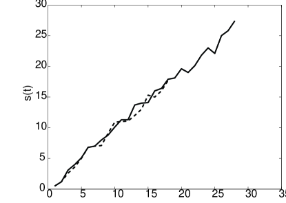
. We see that $s(t)\sim t$, so that the maximum running time to be certain there is no finite box effect should be of the order of the box size: $T\sim L$. Of course it is possible that the effects in question are negligible and we could run for longer, but for the present paper we will be conservative and stop our simulation at $t=L$.

Our simulations are done with box size 120 in units of the initial VV cell size. In the radiation era, we start from conformal time 1, so our dynamic range is 120. In the matter era we use the same box and initial conditions, but the expansion is faster and the simulation is too inaccurate at time 1, so we start from conformal time 2 and thus have dynamic range 60.

IV Results

As in Ref. VOV2 , we characterize the rate of loop production by the function $n(l,t)$ — the number of loops produced per unit loop length per unit volume of the network per unit time. Here we define a loop to be “produced” at the time when it enters a non-self-intersecting trajectory. Thus if a loop is produced from the network and later fragments, we do not count the original loop but only the final fragments in the production function.

In a scaling network VOV2 ,

$$n(l,t)=t^{-5}f(x),$$ (10)

where $f$ can be any function of $x=l/t$. The function $f(x)$ is plotted in Fig. 3

Figure 3: The production rate of loops in the radiation era. Each graph is the loop production rate averaged around the labeled time. The vertical axis is $x^{2}f(x)$, which is the rate of length emitted into loops per logarithmic interval of $x$. Dotted lines are power-law extrapolations of the right side of the first peak, for times (from top to bottom) 45, 60, and 90.

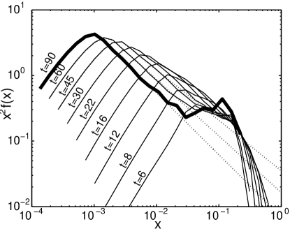
for the radiation era and in Fig. 4

Figure 4: As in Fig. 3 for the matter era.

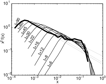
for the matter era. Unlike in the flat-spacetime simulation, where loops smaller than some fraction of the horizon are removed, no artificial cut-off is present in the expanding-universe simulations. String loops are only removed when they are in a non-self-intersecting trajectory. By that time their physical size is much smaller than the interstring distance and they are not likely to interact with the rest of the network.

Scaling in loop production means production of loops at a fixed fraction of the horizon size, and thus a fixed $x$. So a scaling feature in the loop production spectrum is one which appears at a fixed horizontal position in Figs. 3 and 4. Indeed such a feature exists in these figures. At late times a peak appears around $x=0.1$. There is also a (higher) non-scaling peak, which moves to the left as time passes. We believe that this peak is due to the initial conditions, which are not exactly the conditions of a scaling network. In the long run, when the structures on the scales of the initial condition are smoothed out, we expect the non-scaling peak to die away and the scaling peak to dominate the evolution.

The scaling behavior can be seen better if one excludes the loops contributing to the non-scaling peak. We make a power law extrapolation of the non-scaling contribution (presumably an overestimate) to larger values of $x$, shown in Figs. 3 and 4 with dotted lines. Subtracting this extrapolated contribution gives a better view of the scaling peak, shown in Fig. 5.

Figure 5: The scaling peak of the loop production rate with the extrapolated non-scaling peak subtracted, for times (from bottom to top) 45, 60, and 90. The radiation era is shown dashed and the matter era solid. The scaling peak in both cases is very approximately at $x=0.1$.

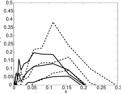
It also worth mentioning that our expansion algorithm becomes more and more exact with time, since $H$ becomes smaller and smaller while the segments of string do not get longer. Therefore, the growth of the scaling peak at late times cannot be attributed to the inaccuracy of the first-order approximation.

V Conclusion

We have presented the results of expanding-universe simulations of a cosmic string network. Our simulations keep the string position and velocity in functional form and have no minimum resolution. They are exact in the flat-spacetime limit; in the expanding universe they use an approximation accurate to first order in the ratio of the string segment size (from the initial conditions) to the Hubble distance.

The loop production is originally dominated by loops whose size results from the initial conditions, but at late times there is a new, scaling peak in the loop production spectrum. The peak value of loop length is about $0.1t$ in flat spacetime, in the radiation era, and in the matter era.

Our simulations run until $t=L$, where $t$ is conformal time and $L$ is the box size, in this case 120 times the initial Vachaspati-Vilenkin cube size. We start at $t=1$ in the radiation era, so the “dynamic range” (final/initial time) is 120, much longer than in other simulations (3 in Ref. MS , 8 in Ref. RSB ). Because of this difference, we are able to see the late time behavior of the string network that is quite different from the initial evolution.

References

- (1) T. W. B. Kibble, J. Phys. A9, 1387 (1976); For a review see A. Vilenkin and E. P. S. Shellard, Cosmic Strings and Other Topological Defects (Cambridge University Press, 2000).
- (2) S. Sarangi and S. H. Tye, Phys. Lett. B536, 185 (2002).
- (3) G. Dvali and A. Vilenkin, JCAP 0403, 010 (2004).
- (4) E. J. Copeland, R. C. Myers and J. Polchinski, JHEP 06, 013 (2004).
- (5) T. W. B. Kibble, Nucl. Phys. B 252, 227 (1985) [Erratum-ibid. B 261, 750 (1985)].
- (6) D. P. Bennett, Phys. Rev. D 34, 3592 (1986).
- (7) A. Albrecht and N. Turok, Phys. Rev. Lett. 54, 1868 (1985); Phys. Rev. D 40, 973 (1989).
- (8) D. P. Bennett and F. R. Bouchet, Phys. Rev. Lett. 60, 257 (1988); 63, 2776 (1989); Phys. Rev. D 41, 2408 (1990).
- (9) B. Allen and E. P. S. Shellard, Phys. Rev. Lett. 64, 119 (1990)
- (10) V. Vanchurin, K. Olum and A. Vilenkin, Phys. Rev. D 72, 063514 (2005)
- (11) V. Vanchurin, K. D. Olum and A. Vilenkin, Phys. Rev. D 74, 063527 (2006)
- (12) A. Vilenkin, Phys. Rev. Lett. 46, 1169 (1981)
- (13) T. W. B. Kibble, Nucl. Phys. B252, 227 (1985).
- (14) C. J. A. P. Martins and E. P. S. Shellard, Phys. Rev. D 73, 043515 (2006)
- (15) C. Ringeval, M. Sakellariadou and F. Bouchet, JCAP 0702, 023 (2007)
- (16) T. Vachaspati and A. Vilenkin, Phys. Rev. D 30, 2036 (1984)