Physical mechanisms that shape the morphologies of extragalactic jets

Este documento describe ..

Abstract

In order to find a law characterising the decrease of velocity along a jet, five analytical methods are suggested. The first two simple models examine the variation of velocity in the presence of Newton’s or Stoke’s resistance. The equation that represents the conservation of the momentum along a pyramidal sector is solved from an analytical point of view (third model). The application of the conservation of the total momentum flux allows us to deduce the velocity of the galaxy as a function of time for classical velocities (fourth model) and relativistic velocities (fifth model). The variation of velocity along the jet combined with an adequate composition of jet precession velocity , rotational velocity of the galaxy , and galaxy dispersion velocity in the cluster  allows us to trace the geometrical pattern of the head-tail radio sources. Application of the developed theory/code to the radio galaxies NGC1265,NGC4061,NGC326, and Cygnus A gives the central galaxy’s approximate dispersion velocities in the direction perpendicular to the jet. A transition from head–tails to classical double radio galaxies as a function of the increasing jet’s mechanical power is introduced.

galaxies :jets radio continuum : galaxies

0.1 Introduction

The extra-galactic radio sources are classified on the basis of the position of the brightest radio emitting regions with respect to the channel: FR-I have hot spots that are more distant from the nucleus (typical example Cygnus A) , FR-II radio galaxies have emission uniformly distributed along the channel (typical example 3C449). The physical parameter that governs this classification is the radiated power: the more powerful radio galaxies being classified as FR II,see Fanaroff & Riley (1974) for details. The classification then becomes more complicated in the presence of complex morphologies and two classifications are introduced : NAT ( Narrow Angle Tail) and WAT ( Wide Angle Tail). But a closer look at NGC 1265 reveals that the angle subtended by the two channels is not so ”narrow”, see Figure 1 of  Odea & Owen (1986); possibly, in this case a distinction should be made between internal regions of the channel where the patterns are similar and the extended regions where conversely the division in WAT and NAT is more evident.

For more details on the classification scheme the interested reader is advised to refer to the book by de Young (2002). The X-ray observations of the Galactic black hole XTE J1118+480 are consistent with extended jets being the source of the hard X-ray flux. In this hypothesis the disc would then simply represent a small solid angle as seen from the emission region, see Miller et al. (2002). This point of view is not new and has been explored by Mendoza et al. (2005) who suggested a unified model for quasars and mu-quasars . In general, the shapes seem to be independent from (or weakly correlated to) the cluster parameters, such as physical position in the cluster, number of galaxies, cluster richness, cluster morphology and x-ray emission. Some of the models that can explain the bending of the jets will now be briefly reviewed

• The geometrical models started with Jaffe & Perola (1973) where two models were developed to explain the formation of ”tailed” radio sources like 3C 129. They continued inserting precession and relativistic effects in SS433, see Hjellming & Johnston (1982). An analytical model was presented for the evolution of a powerful double radio source on a small scale , see Alexander (2000).

• Euler’s equation model, where bending is produced by the ram pressure $\rho_{ICM}V_{j}^{2}$ of the intra-cluster medium, is analysed by  Burns & Owen (1980) in order to explain the structure of 1638+538 (4C53.57), and by  Venkatesan et al. (1994) in order to understand the behaviour of NAT in poor clusters of galaxies. Further on, a hydro-dynamical code was built in order to explain the NAT sources, see  Norman et al. (1994). From an observational point of view it is interesting to note that the velocities of the NAT galaxies are inadequate for producing the ram pressure necessary to bend the radio jets, see  Bliton et al. (1998).

• The slingshot ejection model consists in the ejection of black holes from the host galaxy: the bending is obtained from the oscillations about the center of the merged galaxy, see for example  Valtonen & Kotilainen (1989).

• The 3-dimensional magneto-hydrodynamic (MHD) simulations, based on the Sweeping Magnetic-Twist model  Nakamura et al. (2001), produce a wiggled structure of AGN radio jets.

• The interaction between a jet with a stratified cloud, see Raga & Canto (1996), or with a spherically symmetric pressure stratification , see Canto & Raga (1996), can lead to a final configuration in which the jet has bored a hole through the cloud, or large deflections are obtained.

• A jet can generate an internal shock wave by adopting either a non-relativistic framework , see Icke & Hughes (1991) or a relativistic framework, see Mendoza & Longair (2002).

• From a relativistic point of view Mendoza & Longair (2001) showed that bending relativistic jets is much more difficult than bending non-relativistic ones. This is the reason why most FR-II radio galaxies appear straight.

The already cited models concerning the bending leave a series of questions unanswered or partially answered:

• Is it possible to deduce a law of motion in the presence of viscosity in laminar and turbulent jets?

• Is it possible to trace the jet velocity on the basis of physical parameters such as linear density of energy of the radio source and constant density of the IGM (Inter Galactic Medium)?

• Is it possible to develop a consistent theory in which at a given time the jet opening angle increases abruptly?

• Is it possible to include relativistic effects in turbulent jets that generalise the work made by Raga & Canto (1996) and Canto & Raga (1996) on the interaction between a jet and a stratified cloud ?

• Once the main jet trajectory is obtained, could other kinematical components be added such as jet precession, galaxy rotation and galaxy bulk velocity?

• Does the developed theory match the observed patterns traced by the radio sources?

• Could the transition FR-I $\Rightarrow$ FR-II be simulated by increasing the total jet’s luminosity?

In order to answer these questions in Section 0.2 the equations of motion were derived in the presence of Stoke’s law of resistance , Newton’s law of resistance and turbulent eddy viscosity. Some analytical computations on the momentum conservation in an extra-galactic pyramidal sector advancing in a surrounding medium were developed in Section 0.3. In Section 0.4 the theory of the two-phase beam was set up. The theory of the relativistic turbulent jets was developed in Section 0.5. The theory for the composition of the velocities in a head-tail radio source was developed in Section 0.6. The application of the developed theory to well specified radio sources such as NGC1265,NGC4061, NGC326 and Cygnus A was reported in Section 0.7. A power transition is simulated in Section 0.7.5 replacing the energy with the total power in the law of motion. The theory of the Kelvin-Helmholtz instabilities was reviewed and implemented on the radio-sources in Section 0.9.

0.2 Viscosity models

When a laminar jet moves through the IGM or the ISM a retarding drag force $F_{drag}$ is applied. If $v$ is the instantaneous velocity the simplest model which is usually considered is where

$$F_{drag}\propto v^{n}\quad,$$ (1)

with $n$ as an integer. Here the case of $n=1$ and $n=2$ is considered. In classical mechanics $n=1$ is referred to as Stoke’s law of resistance and $n=2$ as Newton’s law of resistance. We now consider two laminar jets and the turbulent case separately.

0.2.1 Stoke’s behaviour

Consider a slice of the jet with mass $m$. The equation of motion is given by

$$m\frac{dv}{dt}=-bv$$ (2)

or

$$\frac{dv}{dt}=-Bv\quad,$$ (3)

where $B=b/m$. The temporal behaviour of the velocity turns out to be

$$v=v_{0}e^{-Bt}\quad,$$ (4)

where $v_{0}$ is the initial velocity. The distance at the time t is

$$x=\frac{v_{0}}{B}(1-e^{-Bt})\quad,$$ (5)

and this can be considered the first law of motion. The velocity space dependence is

$$v-v_{0}=-Bx\quad.$$ (6)

The velocity of the jet is allowed to vary between a maximum value at the beginning (the inner region), $v=v_{0}=\frac{c}{c_{f}}$ with $c_{f}$ a number bigger than one , and a minimum value at the end (the outer region) , for example $v=\frac{c}{10000}$. In this way the coefficient $B$ can be found by identifying x with the jet’s length $x_{1}$

$$B=\frac{v_{0}-c/10000}{x_{1}}\quad.$$ (7)

The lifetime of the radiosource ,$t_{RS}^{Stoke}$, can be derived from equation (4) once the numerical value of $B$ is known

$$t_{RS}^{Stoke}=\frac{ln\frac{v_{0}\times 10000}{c}}{B}\quad,$$ (8)

that becomes

$$t_{RS}^{Stoke}=\frac{ln\frac{10000}{c_{f}}}{B}\quad.$$ (9)

0.2.2 Newton’s behaviour

The equation of motion is now

$$m\frac{dv}{dt}=-av^{2}\quad,$$ (10)

or

$$\frac{dv}{dt}=-Av^{2}\quad,$$ (11)

where $A=a/m$ . The temporal behaviour of the velocity turns out to be

$$v=\frac{v_{0}}{1+v_{0}At}\quad,$$ (12)

and the distance

$$x=\frac{ln(Av_{0}t+1)}{A}\quad,$$ (13)

which can be considered the second law of motion. The velocity space dependence is

$$x=\frac{-ln\leavevmode\nobreak\ \frac{vc_{f}}{c}}{A}\quad.$$ (14)

The coefficient $A$ can be found by inserting $\frac{v}{c}=1/10000$ which corresponds to $v=30\leavevmode\nobreak\ {\mathrm{km/sec}}$ while $L$, the length of the jets, is equal to $x$ , later called $x_{1}$.

Here the lifetime of the radiosource ,$t_{RS}^{Newton}$ , can be derived from equation (12) once the numerical value of $A$ is known

$$t_{RS}^{Newton}=\bigl{(}{\frac{c}{c_{f}v}-1}\bigr{)}\frac{c_{f}}{cA}\quad.$$ (15)

Parameters of the artificial viscosity from a sample of WAT

A sample of 7 radio–galaxies classified as Wide Angle Tails (WAT) was imaged sensitively at high resolution by  Hardcastle & Sakelliou (2004). This sample is here considered as a source of data that allows us to derive the parameters of  Section 0.2.2 and Section 0.2.1, see Table 1. The parameters of the first two laws of motion are found once the averaged velocity at the beginning of the jet (alias $c_{f}$ ) and at the end of the jet are fixed by observational arguments. The spectroscopical measurements are a good candidate to find the jet’s velocity but attention should be paid to the fact that at a given position x the velocity can vary considerably from the boundary to the center of the jet , see formula (21).

Table 1: Artificial viscosity parameters of seven WAT ;
$c_{f}$ = 1.25 and velocity at the end v/c=1/10000. The value of $c_{f}$ is chosen in order to have relativistic velocities in the initial stage (inner region) of the jet .

$$\begin{array}[]{lccccc}\hline\cr\hline\cr\vskip 3.0pt plus 1.0pt minus 1.0pt\cr Radio\leavevmode\nobreak\ name&\mathrm{x_{1}\leavevmode\nobreak\ [{\mathrm{kpc}}]}&t_{RS}^{Stoke}[10^{6}{\mathrm{year}}]&B[1/{\mathrm{year}}]&t_{RS}^{Newton}[10^{6}{\mathrm{year}}]&A[1/\mathrm{pc}]\\ \vskip 3.0pt plus 1.0pt minus 1.0pt\cr\hline\cr\vskip 3.0pt plus 1.0pt minus 1.0pt\cr 0647+693&81&2.9&3.10\leavevmode\nobreak\ 10^{-6}&2.810^{2}&1.1\leavevmode\nobreak\ 10^{-4}\\ \vskip 3.0pt plus 1.0pt minus 1.0pt\cr 1231+674&35&1.25&7.13\leavevmode\nobreak\ 10^{-6}&1.210^{2}&2.56\leavevmode\nobreak\ 10^{-4}\\ \vskip 3.0pt plus 1.0pt minus 1.0pt\cr 1333+412&20&0.79&1.24\leavevmode\nobreak\ 10^{-5}&71&4.49\leavevmode\nobreak\ 10^{-4}\\ \vskip 3.0pt plus 1.0pt minus 1.0pt\cr 1433+674&49&1.76&5\leavevmode\nobreak\ 10^{-6}&1.710^{2}&1.83\leavevmode\nobreak\ 10^{-4}\\ \vskip 3.0pt plus 1.0pt minus 1.0pt\cr 2236-176&44&1.58&5.67\leavevmode\nobreak\ 10^{-6}&1.510^{2}&2.0\leavevmode\nobreak\ 10^{-4}\\ \vskip 3.0pt plus 1.0pt minus 1.0pt\cr 3C465&28&1.0&8.9\leavevmode\nobreak\ 10^{-6}&99&3.2\leavevmode\nobreak\ 10^{-4}\\ \vskip 3.0pt plus 1.0pt minus 1.0pt\cr 1610-608&13&0.46&1.8\leavevmode\nobreak\ 10^{-5}&46&6.9\leavevmode\nobreak\ 10^{-4}\\ \vskip 3.0pt plus 1.0pt minus 1.0pt\cr\vskip 3.0pt plus 1.0pt minus 1.0pt\cr\hline\cr\hline\cr\end{array}$$

0.2.3 Turbulent jets

The theory of turbulent jets emerging from a circular hole can be found in different books with different theories , see Bird et al. (2002), Landau (1987), and Goldstein (1965). The basic assumptions common to the three already cited approaches are

1. The rate of momentum flow , $J$, represented by

   $$J=constant\times\rho b^{2}\overline{v}_{x,max}^{2}\quad,$$ (16)

   is constant; here $x$ is the distance from the initial circular hole , $b(x)$ is the jet’s diameter at distance $x$, $\overline{v}_{x,max}$ is the maximum velocity along the the centerline, $constant$ is

   $$constant=2\pi\int_{0}^{\infty}f^{2}\xi d\xi\quad,$$ (17)

   where

   $$f(\xi)=\frac{\overline{v}_{x}}{\overline{v}_{x,max}}\quad with\quad\xi=\frac{x}{b_{1/2}}\quad,$$ (18)

   and $\rho$ is the density of the surrounding medium see equation (5.6-3) in Bird et al. (2002).

2. The jet’s density $\rho$ is constant over the expansion and equal to that of the surrounding medium.

When omitting the details of the computation, an expression can be found for the average velocity $\overline{v}_{x}$, see equation (5.6-21) in Bird et al. (2002),

$$\overline{v}_{x}=\frac{\nu^{(t)}}{x}\frac{2C_{3}^{2}}{\bigl{[}1+\frac{1}{4}(C_{3}\frac{r}{x})^{2}\bigr{]}^{2}}\quad,$$ (19)

where $\nu^{(t)}$ is the kinematical eddy viscosity and $C_{3}$ , see equation (5.6-23) in Bird et al. (2002),

$$C_{3}={\sqrt{\frac{3}{16\pi}}{\sqrt{\frac{J}{\rho}}}}{\frac{1}{\nu^{(t)}}}\quad.$$ (20)

An important quantity is the radial position , $r=b_{1/2}$ , corresponding to an axial velocity one-half of the centerline value , see equation (5.6-24) in Bird et al. (2002),

$$\frac{\overline{v}_{x}(b_{1/2},x)}{\overline{v}_{x,max}(x)}=\frac{1}{2}=\frac{1}{\bigl{[}1+\frac{1}{4}(C_{3}\frac{b_{1/2}}{x})^{2}\bigr{]}^{2}}\quad.$$ (21)

The experiments in the range of Reynolds number ,$Re$, $10^{4}\leq Re\leq 310^{6}$ (see Reichardt (1942) , Reichardt (1951) and Schlichting (1979)) indicate that

$$b_{1/2}=0.0848x\quad,$$ (22)

and as a consequence

$$C_{3}=15.17\quad,$$ (23)

and therefore

$$\frac{\overline{v}_{x}(r)}{\overline{v}_{x,max}(r)}=\frac{1}{\bigl{[}1+0.414(\frac{r}{b_{1/2}})^{2}\bigr{]}^{2}}\quad.$$ (24)

Figure 1 reports the behaviour of the velocity distribution as given by equation (24).

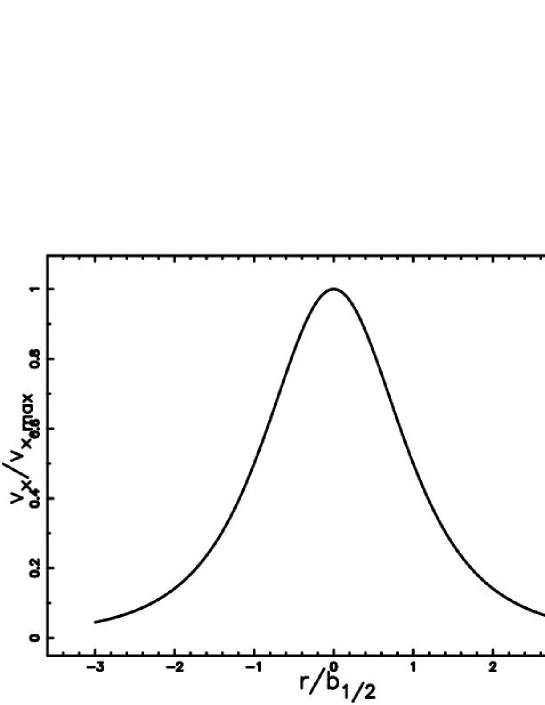
Figure 1: Mean velocity profile vs. channel radius in a circular jet in turbulent flow. The velocity distribution is a function growing from zero (at the wall of the channel) to a maximum value in the central region.

The average velocity, $\overline{v}_{x}$, is $\approx\leavevmode\nobreak\ 1/100$ of the centerline value when $r/b_{1/2}$ = 4.6 and this allows to say that the diameter of the jet is

$$b=2\times 4.6b_{1/2}\quad.$$ (25)

On introducing the opening angle $\alpha$ , the following new relationship is found

$$\frac{\alpha}{2}=\arctan\frac{4.6b_{1/2}}{x}\quad.$$ (26)

The generally accepted relationship between the opening angle and Mach number , see equation (A33) in de Young (2002) , is

$$\frac{\alpha}{2}=\frac{c_{s}}{v_{j}}=\frac{1}{M}\quad,$$ (27)

where $c_{s}$ is the sound velocity, $v_{j}$ the jet’s velocity and $M$ the Mach number. The new relationship (26) replaces the traditional relationship (27). The parameter $b_{1/2}$ can therefore be connected with the jet’s geometry

$$b_{1/2}=\frac{1}{4.6}\tan(\frac{\alpha}{2})x\quad.$$ (28)

If this approximate theory is accepted, equation (22) gives $\alpha=42.61^{\circ}$ : this is the theoretical value that originates the so called Reichardt profiles. The value of $b_{1/2}$ fixes the value of $C_{3}$ and therefore the eddy viscosity is

$$\nu^{(t)}={\sqrt{\frac{3}{16\pi}}{\sqrt{\frac{J}{\rho}}}}{\frac{1}{C_{3}}}={\sqrt{\frac{3}{16\pi}}}{\sqrt{constant}}\;{b{v}_{x,max}}{\frac{1}{C_{3}}}\quad.$$ (29)

In order to continue the integral that appears in $constant$ should be evaluated, see equation (17). The numerical integration gives

$$\int_{0}^{\infty}f^{2}\xi d\xi=0.402\quad,$$ (30)

and therefore

$$constant=2.528\quad.$$ (31)

On introducing typical parameters of jets like $\alpha$=$5^{\circ}$, ${v}_{x,max}$=$v_{100}=v[{\mathrm{km/sec}}]/100$, $b=b_{1}$ where $b_{1}$ is the momentary radius in ${\mathrm{kpc}}$ , it is possible to deduce an astrophysical formula for the kinematical eddy viscosity

$$\nu^{(t)}=0.0028\,b_{1}v_{100}\mathrm{\frac{kpc^{2}}{10^{7}year}}\quad when\quad C_{3}=135.61\quad.$$ (32)

This paragraph concludes underlining the fact that in extragalactic sources it is possible to observe both a small opening angle , $\approx\leavevmode\nobreak\ 5^{\circ}$, see Section 0.7.4 and great opening angles , i.e. $\approx\leavevmode\nobreak\ 34^{\circ}$ in the outer regions of 3C31 Laing & Bridle (2004).

0.3 A continuous model

The jet is now explained as due to a continuous flow in a given direction.

The constrained basic elements of our theory are the mean spread rate of the jet measured on the radio maps , the linear density of energy and the initial jet radius $r_{i}$. The turbulent hyper-sonic flow , Mach number $>$ 6 , is one of the most complicated problems in fluid mechanics. Here the key assumption is that due to the turbulent mass transfer, the density in the jet is the same as the surrounding medium, see for example equation (10.25) in  Hughes & Brighton (1967). This allows the jet law of motion to be expressed in terms of the IGM’s density. We identify our jet with a pyramidal section characterised by a solid angle $\Delta\;\Omega$ and overall length $x_{1}$. From a practical point of view, $\alpha_{0}$ (the first opening angle) is reported in the captions. The solid angle $d\Omega$ in spherical coordinates (r,$\theta,\phi$) is

$$d\Omega=\sin(\theta)d\theta d\phi\quad.$$ (33)

On shifting to the finite differences, the following is obtained

$$\Delta\Omega=(\cos(0)-\cos(\alpha_{0}\frac{2\pi}{360}))(\alpha_{0}\frac{2\pi}{360})\leavevmode\nobreak\ \leavevmode\nobreak\ \mathrm{steradians}\quad,$$ (34)

that when the angles are small becomes

$$\Delta\Omega\approx\frac{1}{2}(\frac{\alpha_{0}2\pi}{360^{\circ}})^{3}\mathrm{steradians}\quad,$$ (35)

where $\alpha_{0}$ represents the limit of the integration and is expressed in degrees.

As an example, when $\alpha_{0}$=$10^{\circ}$, $\Delta\;\Omega=2.65\leavevmode\nobreak\ 10^{-3}\leavevmode\nobreak\ \mathrm{steradians}$. A plot that depicts the assumed geometry is reported in Figure 2.

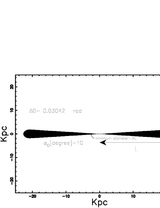
Figure 2: Two dimensional view of the continuous jet; the physical parameters are the same as the simulation of NGC4061 , see Figure 5.

The approximate advancing area of the jet of momentary length $x$, $A_{j}$, will therefore be

$$A_{j}\approx x^{2}\Delta\Omega\quad.$$ (36)

The jet is divided in many slices perpendicular to the direction of motion , each one of thickness $r_{i}$ (the initial radius); the number of slices, $n_{j}$, is therefore

$$n_{j}=NINT(\frac{x_{1}}{r_{i}})\quad,$$ (37)

where NINT denotes the nearest integer. The volume of slice, $V_{s}$, is

$$V_{s}=x^{2}\Delta\Omega r_{i}\quad,\quad$$ (38)

and the mass acquired in a slice from the external medium of a density, $\rho$, is

$$\Delta M=\rho\times V_{s}=\rho x^{2}\Delta\Omega r_{i}\quad.$$ (39)

The hypothesis of a jet in which $\rho$ is constant, is used in the theory of turbulent jets, see Section 0.2.3. The equation that represents the momentum conservation is:

$$\frac{d}{dt}\left(\Delta M\dot{x}\right)=px^{2}\Delta\Omega\quad,$$ (40)

where $p$ is the pressure. In the case of constant density, equation (40) becomes

$$\frac{d}{dt}\left(x^{2}\dot{x}\right)=\frac{px^{2}}{\rho r_{i}}\quad.$$ (41)

The pressure of internal gas decreases according to the adiabatic law

$$p=p_{i}({V_{i}\over V})^{5/3}\quad,$$ (42)

where $V_{i}$ is the volume of the first slice and

$$p_{i}=\frac{2}{3}\frac{\frac{E}{n_{j}}}{V_{i}}\quad.$$ (43)

Under the adiabatic hypothesis, the differential equation (41) is transformed in

$$\frac{d}{dt}\left(x^{2}\dot{x}\right)=Hx^{-4/3}\quad,$$ (44)

where

$$H=\frac{1}{\rho}p_{i}\frac{1}{r_{i}^{-7/3}\Delta\Omega^{5/3}}\quad,$$ (45)

and

$$p_{i}=\frac{\frac{2}{3}E}{x_{1}r_{i}^{2}}\quad.$$ (46)

To integrate this equation, $x^{2}\dot{x}=Ax^{\alpha}$ is used. After adopting the initial condition of $x=0$ at $t=0$ and assuming $\rho$ is constant, the equation representing the third law of motion is obtained

$$x=\left(\frac{13}{18}\frac{(3\alpha+4)}{\alpha}Ht^{2}\right)^{3/13}\quad,$$ (47)

and since $\alpha=5/6$ :

$$x=\left(\frac{507}{90}Ht^{2}\right)^{3/13}\quad.$$ (48)

The velocity of the jet turns out to be:

$$v(t)={\dot{x}}=\frac{6}{13}\frac{x}{t}\quad.$$ (49)

The astrophysical quantities can now be introduced

$$x(t)=2.541\,{\mathrm{kpc}}\,\left({\frac{{{\it t_{7}}}^{2}{\it E_{56}}\,\sqrt[3]{{\it r_{i}^{1}}}}{{\it x_{1}^{1}}\,{\Delta\Omega}^{5/3}{\it n_{0}}}}\right)^{3/13}\quad,$$ (50)

where $E_{56}$ =$E/10^{56}$ ergs , $r_{i}^{1}=r_{i}/1{\mathrm{kpc}}$ , $x_{1}^{1}=x_{1}/1{\mathrm{kpc}}$ , $t_{7}$ = $t/(10^{7})$ year and $\rho$ = $n_{0}\leavevmode\nobreak\ m_{H}$ with $n_{0}$ representing the number of particles in a cubic centimetre and $m_{H}$ the hydrogen mass. A similar formula is deduced for the velocity

$$\dot{R}=114.92\,{\mathrm{\frac{km}{s}}}\,\left({\frac{{\it E_{56}}\,\sqrt[3]{{\it r_{i}^{1}}}}{{\it x_{1}^{1}}\,{\Delta\Omega}^{5/3}{\it n_{0}}}}\right)^{3/13}t_{7}^{-7/13}\quad.$$ (51)

In the case of SNR a comparison can be made with the radius $R(t)\propto\leavevmode\nobreak\ t^{2/7}$ of the adiabatic phase of the SNR , see for example  McCray & Layzer (1987) , and with $R(t)\propto\leavevmode\nobreak\ t^{2/5}$ of the so called Sedov solution , see Sedov (1959) and Landau (1987):

$$R(t)=\bigl{(}{\frac{25}{4}}\,{\frac{{\it E}\,{t}^{2}}{\pi\,\rho}}\bigr{)}^{1/5}\quad,$$ (52)

where $t$ represents the time, $E$ is the energy injected in the explosion, and $\rho$ is the density of matter. When the jets are analyzed a comparison can be made with the solution presented in Kaiser & Alexander (1997). In their model the density $\rho_{x}$ of the gas surrounding the jets scales as

$$\rho_{x}=\rho_{0}(\frac{d}{a_{0}})^{-\beta}\quad,$$ (53)

where $d$ is the radial distance from the core of the source , $\rho_{0}$ is the initial density , $a_{0}$ is the scale length and $\beta$ a parameter comprised between 0 and 2. Their length of the jet $L_{j}$ scales as

$$L_{j}\propto t^{3/5-\beta}\quad,$$ (54)

and explains the division between FRI and FRII objects in jet power.

0.4 Two–phase continuous model

The starting point is the conservation of the momentum’s flux in a ”turbulent jet” as outlined in Landau (1987) (pag. 147). The initial point is characterised by the following section :

$$A_{0}=\pi\leavevmode\nobreak\ r_{0}^{2}\quad.$$ (55)

Once $\alpha_{0}$ the first opening angle , $x_{0}$ the initial position on the $x$–axis and $v_{0}$ the initial velocity are introduced, section $A$ at position $x$ is

$$A(x)=\pi\bigl{(}{\it r_{0}}+\left(x-{\it x_{0}}\right)\tan\left((1/2)\,\alpha_{{0}}\right)\bigr{)}^{2}\quad.$$ (56)

The conservation of the total momentum flux states that

$$\rho v_{0}^{2}A_{0}=\rho v(x)^{2}A(x)\quad,$$ (57)

where $v(x)$ is the velocity at position $x$ . The previous equation is valid if the pressure along the jet is constant and viscosity effects are either not considered or have the same effect in the whole momentum flux along the jet. Due to the turbulent transfer, the density $\rho$ is the same on both the two sides of equation (57). The trajectory of the jet as a function of the time is easily deduced from equation (57)

$$x=-{\frac{-{\it x_{0}}\,\tan\left((1/2)\,\alpha_{{0}}\right)+{\it r_{0}}-\sqrt{{\it r_{0}}\,\left({\it r_{0}}+2\,\tan\left((1/2)\,\alpha_{{0}}\right){\it v_{0}}\,t\right)}}{\tan\left((1/2)\,\alpha_{{0}}\right)}}\quad,$$ (58)

and this can be considered the fourth law of motion.

The velocity turns out to be

$${\it v(t)}={\frac{{\it v_{0}}\,{\it r_{0}}}{\sqrt{{\it r_{0}}\,\left({\it r_{0}}+2\,\tan\left((1/2)\,\alpha_{{0}}\right){\it v_{0}}\,t\right)}}}\quad.$$ (59)

In the applications of equation (58) and (59) $r_{0}$ , $r$ , $x_{0}$ and $x$ will be expressed in $\mathrm{kpc}$ , the time $t$ in units of $10^{7}\leavevmode\nobreak\ {\mathrm{year}}$ , $v_{0}$ and $v(x)$ in $\mathrm{\frac{kpc}{10^{7}\leavevmode\nobreak\ year}}$. The velocity $v_{0}$ can be parametrised as a function of the light velocity c as $v_{0}=\frac{c}{c_{f}}$ where $c_{f}$ is an input parameter allowed to vary between 1.2 and 10.

It is now possible to introduce the two phase beam in which , due to a certain physical phenomena, for example the evolution of the K-H instabilities , the beam abruptly increases the opening angle that from $\alpha_{0}$ (first opening angle) becomes $\alpha_{1}$ (second opening angle). This phenomena happens at a given time $t_{1}$ ( $t_{1}\leavevmode\nobreak\ <\leavevmode\nobreak\ t_{2}$ ) and a corresponding length $x_{1}$ ( $x_{1}\leavevmode\nobreak\ <\leavevmode\nobreak\ x_{2}$): here $t_{2}$ denotes the age of the radio-source and $x_{2}$ its global length. In this second phase the trajectory is

$$x=-{\frac{-{\it x_{1}}\,\tan\left((1/2)\,\alpha_{{1}}\right)+{\it r1}-\sqrt{{\it r1}\,\left({\it r1}+2\,\tan\left((1/2)\,\alpha_{{1}}\right){\it v_{1}}\,(t-t_{1})\right)}}{\tan\left((1/2)\,\alpha_{{1}}\right)}}\quad,$$ (60)

and the velocity

$${\it v(t)}={\frac{{\it v_{1}}\,{\it r_{1}}}{\sqrt{{\it r_{1}}\,\left({\it r_{1}}+2\,\tan\left((1/2)\,\alpha_{{1}}\right){\it v_{1}}\,(t-t_{1})\right)}}}\quad.$$ (61)

0.5 Two–phase relativistic model

The starting point is the energy momentum tensor ,$T^{ik}$,

$$T^{ik}=wu^{i}u^{k}-pg^{ik}\quad,$$ (62)

where $u^{i}$ is the 4-velocity , $i$ varies from 0 to 3 , $w$ is the enthalpy for unit volume , $p$ is the pressure and $g^{ik}$ the inverse metric of the manifold, see Landau (1987). The condition for momentum conservation in the presence of velocity , $v$, along one direction states that

$$(w(\frac{v}{c})^{2}\frac{1}{1-\frac{v^{2}}{c^{2}}}+p)A=cost\quad,$$ (63)

where $A$ is the considered area in the direction perpendicular to the motion. The enthalpy for unit volume is

$$w=c^{2}\rho+p\quad,$$ (64)

where $\rho$ is the density , and $c$ the light velocity. The reader may be puzzled by the $\Gamma^{2}$ factor in equation (63), where $\Gamma^{2}=\frac{1}{1-\frac{v^{2}}{c^{2}}}$. However it should be remembered that $w$ is not an enthalpy, but an enthalpy per unit volume: the extra $\Gamma$ factor arises from ”length contraction” in the direction of motion.

With the assumption of turbulent jets ,$p=0$ , the momentum conservation law is obtained

$$(\rho v^{2}\frac{1}{1-\frac{v^{2}}{c^{2}}})A=cost\quad.$$ (65)

This equation is equal to equation (A.32) , the jet ”thrust”, in  de Young (2002). Note the similarity between the previous formula and condition (135.2) in Landau (1987) concerning the shock waves : when $A$=1 they are equals.

In two sections of the jet we have :

$$\rho\,{{\it v_{0}}}^{2}\pi\,{{\it r_{0}}}^{2}{\frac{1}{1-{\frac{{{\it v_{0}}}^{2}}{{c}^{2}}}}}=\rho\,{v}^{2}\left((\pi\,{{\it r_{0}}}^{2}+\pi\,{\it r_{0}}\,x\alpha_{0}+O\left({\alpha_{0}}^{2}\right))\right){\frac{1}{1-{\frac{{v}^{2}}{{c}^{2}}}}}\quad,$$ (66)

where $v$ is the velocity at position $x$, $v_{0}$ the velocity at $x$=0 , $c$ the light velocity and $\alpha_{{0}}$ the opening angle of the jet. Also here due to the turbulent transfer, the density $\rho$ is the same on both sides of equation (66) and the following second degree equation in $\beta=\frac{v}{c}$ is obtained:

$${{\it\beta}}^{2}{\it r_{0}}+{{\it\beta}}^{2}x\alpha_{0}-{{\it\beta}}^{2}{{\it\beta_{0}}}^{2}x\alpha_{0}-{{\it\beta_{0}}}^{2}{\it r_{0}}=0$$ (67)

where $\beta_{0}=\frac{v_{0}}{c}$. The positive solution is :

$$\beta={\frac{\sqrt{{\it r_{0}}}{\it\beta_{0}}}{\sqrt{{\it r_{0}}+x\alpha_{0}-{{\it\beta_{0}}}^{2}x\alpha_{0}}}}\quad.$$ (68)

From equation (68) it is possible to deduce the distance $x_{1/2}$ after which the velocity is half of the initial value:

$$x_{1/2}=-3\,{\frac{{\it r_{0}}}{\alpha_{0}\,\left(-1+{{\it\beta_{0}}}^{2}\right)}}\quad.$$ (69)

In FR-II’s radio-galaxies the velocity is thought to be relativistic until termination at hot-spots; formula (69) states that the typical distance over which the jet is relativistic is a function of the three parameters $\alpha_{0}$ , $r_{0}$ and $\beta_{0}$.

The trajectory of the relativistic jet as a function of the time can be deduced from equation ( 68) and is

$$\int_{0}^{x}\frac{1}{{\frac{\sqrt{{\it r_{0}}}{\it\beta_{0}}}{\sqrt{{\it r_{0}}+x\alpha_{0}-{{\it\beta_{0}}}^{2}x\alpha_{0}}}}}dx=ct\quad.$$ (70)

On integrating it is possible to obtain the equation of the trajectory

$$2/3\,{\frac{{{\it r_{0}}}^{3/2}-\left({\it r_{0}}+x\alpha_{0}-{{\it\beta_{0}}}^{2}x\alpha_{0}\right)^{3/2}}{\alpha_{0}\,\left(-1+{{\it\beta_{0}}}^{2}\right)\sqrt{{\it r_{0}}}{\it\beta_{0}}}}-ct=0\quad.$$ (71)

After some manipulation equation (71) becomes

$$\left(-3\,{\alpha_{0}}^{3}{{\it\beta_{0}}}^{2}+3\,{\alpha_{0}}^{3}{{\it\beta_{0}}}^{4}-{{\it\beta_{0}}}^{6}{\alpha_{0}}^{3}+{\alpha_{0}}^{3}\right){x}^{3}+$$

$$\left(3\,{\it r_{0}}\,{\alpha_{0}}^{2}-6\,{\it r_{0}}\,{\alpha_{0}}^{2}{{\it\beta_{0}}}^{2}+3\,{\it r_{0}}\,{{\it\beta_{0}}}^{4}{\alpha_{0}}^{2}\right){x}^{2}+$$

$$\left(-3\,{{\it r_{0}}}^{2}{{\it\beta_{0}}}^{2}\alpha_{0}+3\,{{\it r_{0}}}^{2}\alpha_{0}\right)x-$$

$$9/4\,{c}^{2}{t}^{2}{\alpha_{0}}^{2}{\it r_{0}}\,{{\it\beta_{0}}}^{6}-3\,{{\it r_{0}}}^{2}ct\alpha_{0}\,{\it\beta_{0}}+3\,{{\it r_{0}}}^{2}ct\alpha_{0}\,{{\it\beta_{0}}}^{3}-$$

$$9/4\,{c}^{2}{t}^{2}{\alpha_{0}}^{2}{\it r_{0}}\,{{\it\beta_{0}}}^{2}+9/2\,{c}^{2}{t}^{2}{\alpha_{0}}^{2}{\it r_{0}}\,{{\it\beta_{0}}}^{4}=0\quad.$$ (72)

The parameter $p$ , see Appendix .11, that regulates the solutions of the cubic equation is now evaluated. When the equation (72) is considered we have $p=0$ and therefore we have one real root that is (the fifth law of motion ) :

$$x(t)=-1/2\,{\frac{-2\,{\it r_{0}}+\sqrt[3]{2}\sqrt[3]{{\it r_{0}}}\left(2\,{\it r_{0}}+3\,ct\alpha_{0}\,{\it\beta_{0}}-3\,ct\alpha_{0}\,{{\it\beta_{0}}}^{3}\right)^{2/3}}{\alpha_{0}\,\left(-1+{{\it\beta_{0}}}^{2}\right)}}\quad.$$ (73)

The velocity of the relativistic jet as function of the time is

$$v(t)={\frac{c{\it\beta_{0}}\,\sqrt[3]{{\it r_{0}}}\sqrt[3]{2}}{\sqrt[3]{2\,{\it r_{0}}+3\,ct\alpha_{0}\,{\it\beta_{0}}-3\,ct\alpha_{0}\,{{\it\beta_{0}}}^{3}}}}\quad.$$ (74)

The velocity $v_{0}$ can be parametrised as a function of the parameter $\beta_{0}$ , a parameter allowed to vary between 0.1 and 0.99999. The two previous equations can be expressed in astrophysical units once $r_{0}^{1}=r_{0}/1{\mathrm{kpc}}$ and $t_{7}$ = $t/(10^{7}\mathrm{year})$ are introduced

$$x(t)=1/2\,{\frac{2\,{\it r_{0}^{1}}-\sqrt[3]{2}\sqrt[3]{{\it r_{0}^{1}}}\left(2\,{\it r_{0}^{1}}+9180.0\,{\it t_{7}}\,\alpha\,{\it\beta_{0}}-9180.0\,{\it t_{7}}\,\alpha\,{{\it\beta_{0}}}^{3}\right)^{2/3}}{\alpha\,\left(-1+{{\it\beta_{0}}}^{2}\right)}}{\mathrm{kpc}}\quad,$$ (75)

and

$$v(t)=299788.2\,{\frac{{\it\beta_{0}}\,\sqrt[3]{{\it r_{0}^{1}}}\sqrt[3]{2}}{\sqrt[3]{2\,{\it r_{0}^{1}}+9180.0\,{\it t_{7}}\,\alpha\,{\it\beta_{0}}-9180.0\,{\it t_{7}}\,\alpha\,{{\it\beta_{0}}}^{3}}}}{\mathrm{\frac{km}{s}}}\quad.$$ (76)

The transition from relativistic to classical velocity is still represented by formulas (60) and (61) but $x_{1}$,$r_{1}$ and $v_{1}$ are the parameters at the end of the relativistic phase.

0.6 The change of framework

The wide spectrum of observed morphologies that characterises the head–tail radio galaxies could be due to the kinematical effects as given by the composition of the velocities in different kinematical frameworks such as decreasing jet velocity , jet precession, rotation, and proper velocity of the host galaxy in the cluster. These effects were partially analysed in  Zaninetti (1989) ; here part of the developed theory and symbols will be used, and will now be briefly reviewed in order to represent the law of motion through a matrix. Of particular interest is the evaluation of various matrices that will enable us to cause transformation from the inertial coordinate system of the jet to the coordinate system in which the host galaxy is moving in space. The various coordinate systems will be ${\bf x}$=$(x,y,z$) , ${\bf x}^{(1)}$=$(x^{(1)},y^{(1)},z^{(1)})$ , $\ldots$ ${\bf x}^{(5)}$=$(x^{(5)},y^{(5)},z^{(5)})$. The vector representing the motion of the jet will be represented by the following $1\times 3$ matrix

$$G=\left[\begin{array}[]{c}0\\ \vskip 6.0pt plus 2.0pt minus 2.0pt\cr 0\\ \vskip 6.0pt plus 2.0pt minus 2.0pt\cr{\it L(t)}\end{array}\right]\quad,$$ (77)

where the jet motion L(t) is considered along the z-axis.

The jet axis, $z$, is inclined at an angle $\Psi_{prec}$ relative to an axis $z^{(1)}$ and therefore the $3\times 3$ matrix, representing a rotation through the x axis, is given by:

$$F=\left[\begin{array}[]{ccc}1&0&0\\ \vskip 6.0pt plus 2.0pt minus 2.0pt\cr 0&\cos\left(\Psi_{prec}\right)&\sin\left(\Psi_{prec}\right)\\ \vskip 6.0pt plus 2.0pt minus 2.0pt\cr 0&-\sin\left(\Psi_{prec}\right)&\cos\left(\Psi_{prec}\right)\end{array}\right]\quad.$$ (78)

From a practical point of view $\Psi_{prec}$ can be derived by measuring the half opening angle of the maximum of the sinusoidal oscillations (named wiggles) that characterises the jet.

If the jet is undergoing precession around the $z^{(1)}$ axis, $\Omega_{prec}$ can be the angular velocity of precession expressed in $\mathrm{radians}$ per unit time ; $\Omega_{prec}$ is computed from the radio maps by measuring the number of sinusoidal oscillations that characterise the jet. The transformation from the coordinates ${\bf x}^{(1)}$ fixed in the frame of the precessing jet to the non-precessing coordinate ${\bf x}^{(2)}$ is represented by the $3\times 3$ matrix

$$E=\left[\begin{array}[]{ccc}\cos\left(\Omega_{prec}\,t\right)&\sin\left(\Omega_{prec}\,t\right)&0\\ \vskip 6.0pt plus 2.0pt minus 2.0pt\cr-\sin\left(\Omega_{prec}\,t\right)&\cos\left(\Omega_{prec}\,t\right)&0\\ \vskip 6.0pt plus 2.0pt minus 2.0pt\cr 0&0&1\end{array}\right]\quad.$$ (79)

The arbitrary orientation of the precession axis relative to the central galaxy at rest, necessitates a transformation from the coordinate frame ${\bf x}^{(2)}$ to the frame ${\bf x}^{(3)}$. The relative orientations are assumed to be characterised by the Euler angles $(\Phi_{j},\Theta_{j},\Psi_{j})$. There is not uniform agreement on the designation of the Euler angles and the manner in which they are generated. We have chosen here to use the conventions found in  Goldstein et al. (2002) and the $3\times 3$ matrix , $D_{E}$, is

$$D_{E}=$$ (80)

$$\left[\matrix{cos\Psi_{j}cos\Phi_{j}-cos\Theta_{j}sin\Phi_{j}sin\Psi_{j}&cos\Psi_{j}sin\Phi_{j}+cos\Theta_{j}cos\Phi_{j}sin\Psi_{j}&sin\Psi_{j}sin\Theta_{j}\cr-sin\Psi_{j}cos\Phi_{j}-cos\Theta_{j}sin\Phi_{j}cos\Psi_{j}&-sin\Psi_{j}sin\Phi_{j}+cos\Theta_{j}cos\Phi_{j}cos\Psi_{j}&cos\Psi_{j}sin\Theta_{j}\cr sin\Theta_{j}sin\Phi_{j}&-sin\Theta_{j}cos\Phi_{j}&cos\Theta_{j}\cr}\right]\quad.$$

On assuming that $\Phi_{j}$= $0^{\circ}$ , $\Psi_{j}$= $0^{\circ}$ and $\Theta_{j}$= $90^{\circ}$  we have the simple expression

$$D_{E}=\left[\begin{array}[]{ccc}1&0&0\\ \vskip 6.0pt plus 2.0pt minus 2.0pt\cr 0&0&1\\ \vskip 6.0pt plus 2.0pt minus 2.0pt\cr 0&-1&0\end{array}\right]\quad.$$ (81)

Another $3\times 3$ matrix is introduced which represents the transformation from $(\bf{x}^{3})$ to $(\bf{x}^{4})$ and defined by a rotation through the axis $z^{(3)}$ of an angle $\Omega_{G}t$ where $\Omega_{G}$ is the angular velocity of the galaxy expressed in $\mathrm{radians}$/time units; the total angle of rotation of the galaxy being $\alpha$ = $\Omega_{G}\;t_{max}$ :

$$C=\left[\begin{array}[]{ccc}\cos\left(\Omega_{G}\,t\right)&\sin\left(\Omega_{G}\,t\right)&0\\ \vskip 6.0pt plus 2.0pt minus 2.0pt\cr-\sin\left(\Omega_{G}\,t\right)&\cos\left(\Omega_{G}\,t\right)&0\\ \vskip 6.0pt plus 2.0pt minus 2.0pt\cr 0&0&1\end{array}\right]\quad.$$ (82)

In the astrophysical applications $\Omega_{G}=0$ because the rotation period of a typical elliptical galaxy is less than the lifetime of a typical radio source; only in the case of NGC326 $\Omega_{G}\leavevmode\nobreak\ \neq\leavevmode\nobreak\ 0$, see discussion in Section 0.7.3.

The last translation represents the change of framework from $\bf(x^{(4)})$, which is co-moving with the host galaxy, to a system $\bf(x^{(5)})$ in comparison to which the host galaxy is in uniform motion. It should be remembered that the dispersion velocity in the cluster (not to be confused with the recession velocity) is $\approx$ 600 ${\mathrm{km/sec}}$ , see Table 1 in  Venkatesan et al. (1994) . The relative motion of the origin of the coordinate system $(x^{(4)},y^{(4)},z^{(4)})$ is defined by the Cartesian components of the galactic velocity ${\bf v_{G}}$, and the required $1\times 3$ matrix transformation representing this translation is:

$$B=\left[\begin{array}[]{c}v\_x\\ \vskip 6.0pt plus 2.0pt minus 2.0pt\cr v\_y\\ \vskip 6.0pt plus 2.0pt minus 2.0pt\cr{\it v\_z}\,t\end{array}\right]\quad.$$ (83)

On assuming, for the sake of simplicity, that $v_{y}$=0 and $v_{x}$=0, the translation matrix becomes:

$$B=\left[\begin{array}[]{c}0\\ \vskip 6.0pt plus 2.0pt minus 2.0pt\cr 0\\ \vskip 6.0pt plus 2.0pt minus 2.0pt\cr{\it v\_z}\,t\end{array}\right]\quad.$$ (84)

In other words, the direction of the galaxy motion in the IGM and the direction of the jet are perpendicular. From a practical point of view the galaxy velocity can be measured by dividing the length of the radio galaxy in a direction perpendicular to the initial jet velocity by the lifetime of the radio source; an example of such measurement is reported in Section 0.8.2.

The final $1\times 3$ matrix $A$ representing the “motion law” can be found by composing the six matrices already described

$$A=B+(C\cdot D_{E}\cdot E\cdot F\cdot G)$$

$$= \left[\begin{array}[]{c}\left(\cos\left(\Omega_{G}\,t\right)\sin\left(\Omega_{prec}\,t\right)\sin\left(\Psi_{prec}\right)+\sin\left(\Omega_{G}\,t\right)\cos\left(\Psi_{prec}\right)\right){\it L(t)}\\ \vskip 6.0pt plus 2.0pt minus 2.0pt\cr\left(-\sin\left(\Omega_{G}\,t\right)\sin\left(\Omega_{prec}\,t\right)\sin\left(\Psi_{prec}\right)+\cos\left(\Omega\,{\it galaxy}\,t\right)\cos\left(\Psi_{prec}\right)\right){\it L(t)}\\ \vskip 6.0pt plus 2.0pt minus 2.0pt\cr{\it v\_z}\,t-\sin\left(\Psi_{prec}\right)\cos\left(\Omega_{prec}\,t\right){\it L(t)}\end{array}\right]\quad.$$ (88)

The three components of the previous $1\times 3$ matrix $A$ represent the jet motion along the Cartesian coordinates as given by the observer that sees the galaxy moving in uniform motion.

0.7 Application of the continuous model

The continuous beam model developed in Section 0.3 is basically represented by equations (50) and (51) and can be easily implemented in a code; this is now applied to various radio–sources.

An attempt to reproduce the mechanical power dependence in the jet trajectory is carried out in Section 0.7.5.

0.7.1 The first part of NGC1265

The first target chosen for our simulation was the radio source NGC1265 at 6 cm. Some basic input parameters extracted from  Odea & Owen (1986) are reported in Table 2.

Table 2: The data from the radio map of NGC1265

$$\begin{array}[]{cc}\hline\cr\hline\cr\vskip 3.0pt plus 1.0pt minus 1.0pt\cr\mathrm{L_{rad}[ergs/sec]}&mean\leavevmode\nobreak\ spread\leavevmode\nobreak\ rate[degree]\\ \vskip 3.0pt plus 1.0pt minus 1.0pt\cr\hline\cr\vskip 3.0pt plus 1.0pt minus 1.0pt\cr 1.110^{40}&10\\ \vskip 3.0pt plus 1.0pt minus 1.0pt\cr\vskip 3.0pt plus 1.0pt minus 1.0pt\cr\hline\cr\hline\cr\end{array}$$

The result of the simulation is reported in Figure 3 and in Figure 4 with the radio map superimposed on the simulation ; the adopted input parameters are given in the caption.

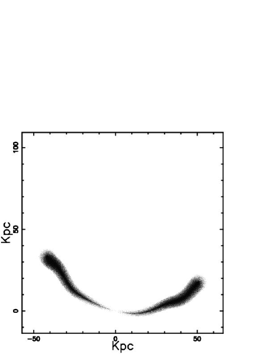
Figure 3: Continuous three-dimensional trajectory of NGC1265: the three Eulerian angles (English notation) characterising the point of view are $\Phi$= 80 ^∘ , $\Theta$= 80 ^∘ and $\Psi$= 10 ^∘. The precession is characterised by the angle $\Psi_{prec}$= 2 ^∘ and by the angular velocity $\Omega_{prec}$= 54.00 [${}^{\circ}/10^{7}\mathrm{year}$]. The three Eulerian angles are: $\Phi_{j}$= 0 ^∘ , $\Psi_{j}$= 0 ^∘ and $\Theta_{j}$= 90 ^∘. The angle of rotation of the galaxy is $\alpha_{G}$= 0 ^∘. The physical parameters characterising the jet motion are : $E_{56}$= 0.02, $t_{1}$= 10.00 $10^{7}\mathrm{year}$, $n_{0}$= 0.01 $\mathrm{particles/cm^{3}}$, $x_{1}$= 18.00 ${\mathrm{kpc}}$ , $r_{i}$= 0.90 ${\mathrm{kpc}}$ , $\alpha_{0}$= 10 ^∘.

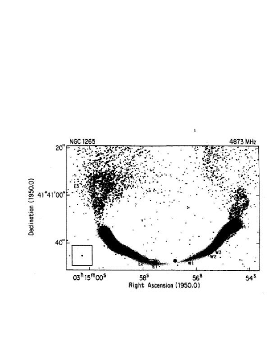
Figure 4: Figure 1 of  Odea & Owen (1986) representing NGC1265 at 4873 MHz superimposed on the theoretical trajectory represented by Figure 3.

The output data as obtained from the code concerning the overall jet length, the perpendicular-displacement, and the galaxy velocity of NGC1265 are reported in Table 3.

Table 3: The physical parameters as output of the simulation on NGC1265

$$\begin{array}[]{ccc}\hline\cr\hline\cr\vskip 3.0pt plus 1.0pt minus 1.0pt\cr\mathrm{x_{1}\leavevmode\nobreak\ [{\mathrm{kpc}}]}&v_{z}\leavevmode\nobreak\ [{\mathrm{km/s}}]&\Delta\leavevmode\nobreak\ z[{\mathrm{kpc}}]\\ \vskip 3.0pt plus 1.0pt minus 1.0pt\cr\hline\cr\vskip 3.0pt plus 1.0pt minus 1.0pt\cr 18.7&84.55&10.3\\ \vskip 3.0pt plus 1.0pt minus 1.0pt\cr\vskip 3.0pt plus 1.0pt minus 1.0pt\cr\hline\cr\hline\cr\end{array}$$

0.7.2 The first part of NGC4061

We have chosen the radio source NGC4061 at 21 cm, see Figure 5b in  Venkatesan et al. (1994) for a radio map; the basic data as extracted from the radio observations are reported in Table 4. The result of the simulation is visualised in Figure 5 and in Figure 6 with the radio map superimposed on the simulation ; the caption of the Figure shows the adopted input parameters while the output data are reported in Table 5.

Table 4: The data from the radio map of NGC4061

$$\begin{array}[]{cc}\hline\cr\hline\cr\vskip 3.0pt plus 1.0pt minus 1.0pt\cr\mathrm{L_{rad}[ergs/sec]}&mean\leavevmode\nobreak\ spread\leavevmode\nobreak\ rate[degree]\\ \vskip 3.0pt plus 1.0pt minus 1.0pt\cr\hline\cr\vskip 3.0pt plus 1.0pt minus 1.0pt\cr 0.0610^{40}&10\\ \vskip 3.0pt plus 1.0pt minus 1.0pt\cr\vskip 3.0pt plus 1.0pt minus 1.0pt\cr\hline\cr\hline\cr\end{array}$$

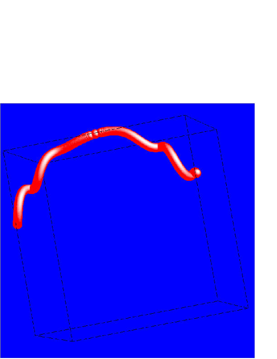
Figure 5: Continuous three-dimensional trajectory of NGC4061: the three Eulerian angles (English notation) characterising the point of view are $\Phi$=100 ^∘ , $\Theta$=-85 ^∘ and $\Psi$=-10 ^∘. The precession is characterised by the angle $\Psi_{prec}$= 5 ^∘ and by the angular velocity $\Omega_{prec}$= 60.00 [${}^{\circ}/10^{7}\mathrm{year}$]. The three Eulerian angles are: $\Phi_{j}$= 0 ^∘ , $\Psi_{j}$= 0 ^∘ and $\Theta_{j}$= 90 ^∘. The angle of rotation of the galaxy is $\alpha_{G}$= 0 ^∘. The physical parameters characterising the jet motion are : $E_{56}$= 0.02, $t_{1}$= 12.00 $10^{7}\mathrm{year}$, $n_{0}$= 0.01 ${\mathrm{particles/cm^{3}}}$, $x_{1}$= 20.00 ${\mathrm{kpc}}$ , $r_{i}$= 1.00 ${\mathrm{kpc}}$ , $\alpha_{0}$= 10 ^∘.

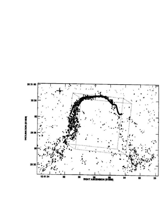
Figure 6: Figure 5b of  Venkatesan et al. (1994) representing NGC4061 at 21cm superimposed on the theoretical trajectory represented by Figure 5.

Table 5: The physical parameters output of the simulation on NGC4061

$$\begin{array}[]{ccc}\hline\cr\hline\cr\vskip 3.0pt plus 1.0pt minus 1.0pt\cr\mathrm{x_{1}\leavevmode\nobreak\ [{\mathrm{kpc}}]}&v_{z}\leavevmode\nobreak\ [{\mathrm{km/s}}]&\Delta\leavevmode\nobreak\ z[{\mathrm{kpc}}]\\ \vskip 3.0pt plus 1.0pt minus 1.0pt\cr\hline\cr\vskip 3.0pt plus 1.0pt minus 1.0pt\cr 20.9&78.65&14.6\\ \vskip 3.0pt plus 1.0pt minus 1.0pt\cr\vskip 3.0pt plus 1.0pt minus 1.0pt\cr\hline\cr\hline\cr\end{array}$$

In this case we know that the dispersion velocity in the cluster is 485${\mathrm{km/sec}}$, see Table 1 in  Venkatesan et al. (1994) .

The velocity $v_{z}$ in our model is 119.08${\mathrm{km/sec}}$ implying an angle of $\approx$ $14.2^{\circ}$ between the direction of the galaxy motion and the initial direction of the jet. A typical plot of the jet velocity as a function of the time is reported in Figure 7.

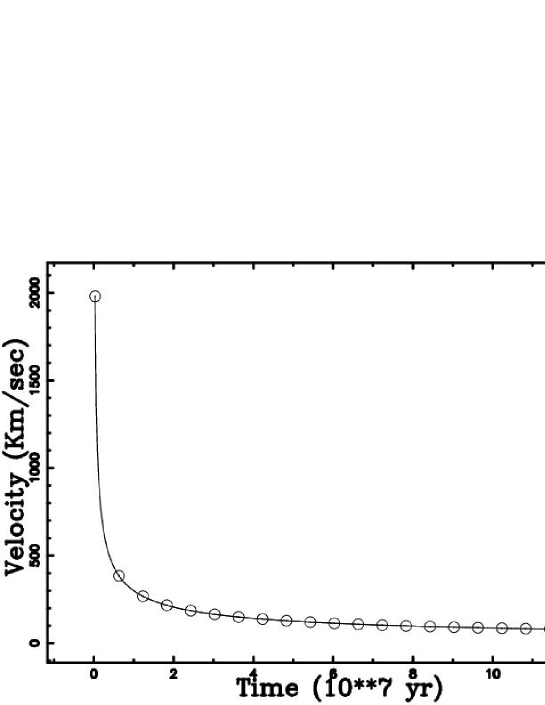
Figure 7: The numerical relationship between velocity and $t_{1}$ in NGC4061. Parameters as in Figure 5.

0.7.3 The first part of NGC326

Another test of our code is the radio galaxy NGC326; in particular we refer to the image at 1.4GHz as given in Figure 6 (bottom panel) of  Murgia et al. (2001) : the basic input data as deduced from the radio map are reported in Table 6.

Table 6: The data from the radio map of NGC326

$$\begin{array}[]{cc}\hline\cr\hline\cr\vskip 3.0pt plus 1.0pt minus 1.0pt\cr\mathrm{L_{rad}[ergs/sec]}&mean\leavevmode\nobreak\ spread\leavevmode\nobreak\ rate[degree]\\ \vskip 3.0pt plus 1.0pt minus 1.0pt\cr\hline\cr\vskip 3.0pt plus 1.0pt minus 1.0pt\cr 0.510^{40}&6.45\\ \vskip 3.0pt plus 1.0pt minus 1.0pt\cr\vskip 3.0pt plus 1.0pt minus 1.0pt\cr\hline\cr\hline\cr\end{array}$$

In this case, the optical observations with HST reveal two cores, one coincident with the origin of the radio galaxy, and the other at the projected distance of 4.8 ${\mathrm{kpc}}$. In this case, it is assumed that the rotation of the host galaxy is due to gravitational interaction; the total angle of rotation being $\alpha_{G}$= $90\leavevmode\nobreak\ ^{\circ}$. Figure 8 reports on the obtained simulation and Figure 9 reports the radio map superimposed on the simulation ; Table 7 gives the data of output from the simulation.

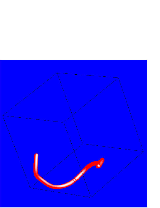
Figure 8: Continuous three-dimensional trajectory of NGC326: the three Eulerian angles (English notation) characterising the point of view are $\Phi$=110 ^∘ , $\Theta$= 65 ^∘ and $\Psi$=-40 ^∘. The precession is characterised by the angle $\Psi_{prec}$= 2 ^∘ and by the angular velocity $\Omega_{prec}$= 51.43 [${}^{\circ}/10^{7}\mathrm{year}$]. The three Eulerian angles are: $\Phi_{j}$= 0 ^∘ , $\Psi_{j}$= 0 ^∘ and $\Theta_{j}$= 90 ^∘. The angle of rotation of the galaxy is $\alpha_{G}$=-90 ^∘. The physical parameters characterising the jet motion are : $E_{56}$= 0.03, $t_{1}$= 14.00 $10^{7}$ $\mathrm{year}$, $n_{0}$= 0.01 ${\mathrm{particles/cm^{3}}}$, $x_{1}$= 30.00 ${\mathrm{kpc}}$ , $r_{i}$= 1.50 ${\mathrm{kpc}}$ , $\alpha_{0}$= 6 ^∘.

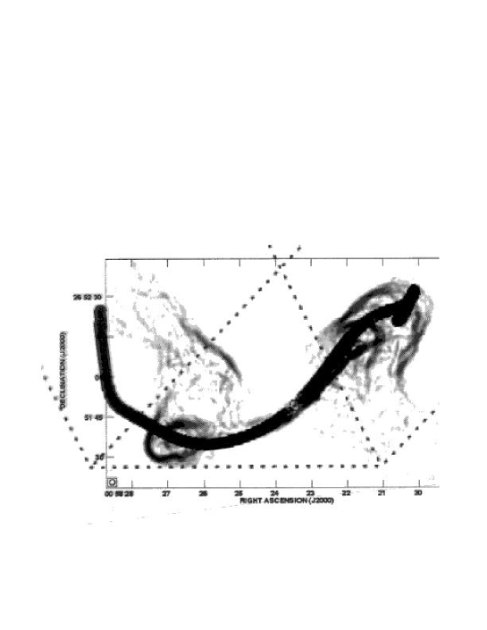
Figure 9: Figure 6 (bottom panel) of   Murgia et al. (2001) superimposed on the theoretical trajectory represented by Figure 8.

Table 7: The physical parameters output of the simulation on NGC326

$$\begin{array}[]{ccc}\hline\cr\hline\cr\vskip 3.0pt plus 1.0pt minus 1.0pt\cr\mathrm{x_{1}\leavevmode\nobreak\ [{\mathrm{kpc}}]}&v_{z}\leavevmode\nobreak\ [{\mathrm{km/s}}]&\Delta\leavevmode\nobreak\ z[{\mathrm{kpc}}]\\ \vskip 3.0pt plus 1.0pt minus 1.0pt\cr\hline\cr\vskip 3.0pt plus 1.0pt minus 1.0pt\cr 30.6&98.71&16.8\\ \vskip 3.0pt plus 1.0pt minus 1.0pt\cr\vskip 3.0pt plus 1.0pt minus 1.0pt\cr\hline\cr\hline\cr\end{array}$$

0.7.4 A sample of WAT

A sample of 7 radio–galaxies has already been presented in Section 0.2.2 and is now considered as a test of the theory developed in Section 0.3. A first look at the radio–maps shows a nearly constant opening angle of $\approx\leavevmode\nobreak\ 5^{\circ}$. On assuming that a constant ratio $E/x_{1}=E_{56}/1{\mathrm{kpc}}=10^{-3}$ characterises the motion, the terminal velocity $v_{1}$ and the age of the jets, $t_{1}$ , see Table 8, can easily be found through an iterative procedure; the length of the jet being provided in Table 7 of    Hardcastle & Sakelliou (2004). From Table 8 the terminal velocities can be compared with the central galaxy dispersion velocity in the cluster.

Table 8: The seven WAT
$\alpha_{0}$=$5^{\circ}$, $r_{i}[{\mathrm{kpc}}]=x_{1}[{\mathrm{kpc}}]/100$,
 $n_{0}=10^{-3}{\mathrm{particles/cm^{3}}}$ and 
$E_{56}/1{\mathrm{kpc}}=10^{-3}$

$$\begin{array}[]{lccc}\hline\cr\hline\cr\vskip 3.0pt plus 1.0pt minus 1.0pt\cr Radio\leavevmode\nobreak\ name&\mathrm{x_{1}\leavevmode\nobreak\ [{\mathrm{kpc}}]}&v_{1}\leavevmode\nobreak\ [{\mathrm{km/s}}]&t_{1}[10^{7}\mathrm{year}]\\ \vskip 3.0pt plus 1.0pt minus 1.0pt\cr\hline\cr\vskip 3.0pt plus 1.0pt minus 1.0pt\cr 0647+693&81&113&32\\ \vskip 3.0pt plus 1.0pt minus 1.0pt\cr 1231+674&35&263&6.0\\ \vskip 3.0pt plus 1.0pt minus 1.0pt\cr 1333+412&20&461&1.95\\ \vskip 3.0pt plus 1.0pt minus 1.0pt\cr 1433+674&49&188&11\\ \vskip 3.0pt plus 1.0pt minus 1.0pt\cr 2236-176&44&209&9.5\\ \vskip 3.0pt plus 1.0pt minus 1.0pt\cr 3C465&28&329&3.8\\ \vskip 3.0pt plus 1.0pt minus 1.0pt\cr 1610-608&13&708&0.82\\ \vskip 3.0pt plus 1.0pt minus 1.0pt\cr\vskip 3.0pt plus 1.0pt minus 1.0pt\cr\hline\cr\hline\cr\end{array}$$

Most of the jets here considered are distinctly one sided over the length modelled, and this fact is here justified by the flip-flop mechanism rather than assuming that they are relativistic over the whole length.

0.7.5 Power transition

The morphological transition between FR–I and FR–II objects can be explained under the assumption of constant power $P$, i.e. negligible synchrotron losses. Equation (50) can be modified by inserting the total power $P=\frac{E}{t}$ and typical parameters of the jet previously adopted such as $\alpha_{0}=5^{\circ}$ and $n_{0}$= 0.001 ${\mathrm{particles/cm^{3}}}$ :

$$x(t_{7})=36.78\,{\mathrm{kpc}}\left({\frac{{{\it t_{7}}}^{3}{\it P_{33}}\,\sqrt[3]{{\it r_{i}}}}{{\it L_{1}}}}\right)^{3/13}\quad,$$ (89)

where $P_{33}=P/10^{33}Watt$. Only the velocity of the host galaxy in the direction perpendicular to that of the jet is here considered

$$y(t_{7})=4.05{\mathrm{kpc}}\;t_{7}\;v_{400}\quad,$$ (90)

where $v_{400}=v[{\mathrm{km/sec}}]/400$. When a comparison of equation (89) and (90) is made, it is clear that an increase in the mechanical power of the galaxy corresponds to an increase in the elongation along x of the phenomena. A typical plot that tentatively reproduces the power transition is reported in Figure 10.

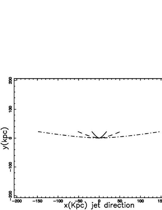
Figure 10: Three jet trajectories as a function of the power. $P_{33}$=100 (dot-dash-dot-dash line) , $P_{33}$=1 (dashed line ) and $P_{33}$=0.01 (continuous line). The other parameters in common to the three trajectories are $\alpha_{0}=5^{\circ}$, $n_{0}$= 0.001 ${\mathrm{particles/cm^{3}}}$, $L_{1}$= 60 , $r_{i}$= $L_{1}$/20 , $t_{7}$=5.0 and $v_{400}$=1. The three Eulerian angles are: $\Phi_{j}$= 0 ^∘ , $\Psi_{j}$= 0 ^∘ and $\Theta_{j}$= 90 ^∘. The three Eulerian angles (English notation) characterising the point of view are $\Phi$= 90 ^∘ , $\Theta$= 90 ^∘ and $\Psi$= 0 ^∘.

There are many ’straight’ FR-I’s, NGC315 is a good example . This can happen when the galaxy’s velocity is lower than the standard value here adopted of 400${\mathrm{km/s}}$ or from a particular point of view of the observer.

0.8 Application of the two–phase beam

The two–phase beam developed in Sections 0.4 and  0.5 is now applied to two radio-sources : in one ,Cygnus A, the relativistic–classic transition is applied and in the other ,0647+693, the classic–classic transition.

0.8.1 Relativistic Cygnus A

A good introduction to the classical double radio sources , as well as to Cygnus A, can be found in chapter 6 of  de Young (2002) . The main physical parameters characterising the jet in Cygnus A , as presented in  Perley et al. (1984b) , are summarised in Table 9; here $x_{1}^{obs}$ is the distance between nucleus and hot-spots , $\alpha_{0}^{obs}$ is the first opening angle (measured on the radio map) and $t_{age}^{obs}$ , the age of the radio–galaxy, as deduced on the basis of the spectral steepening of the lobe emission.

Table 9: The observed data on Cygnus A

$$\begin{array}[]{cccc}\hline\cr\hline\cr\vskip 3.0pt plus 1.0pt minus 1.0pt\cr x_{1}^{obs}\leavevmode\nobreak\ [{\mathrm{kpc}}]&\alpha_{0}^{obs}\leavevmode\nobreak\ [^{\circ}]&t_{age}^{obs}[10^{7}\mathrm{year}]\\ \vskip 3.0pt plus 1.0pt minus 1.0pt\cr\hline\cr\vskip 3.0pt plus 1.0pt minus 1.0pt\cr 60&5&0.6\\ \vskip 3.0pt plus 1.0pt minus 1.0pt\cr\vskip 3.0pt plus 1.0pt minus 1.0pt\cr\hline\cr\hline\cr\end{array}$$

Once the $t_{2}=t_{age}^{obs}$ is inserted in the code, the other input parameters are varied in order to obtain $x_{1}\leavevmode\nobreak\ \approx x_{1}^{obs}$; this is obtained by solving numerically the integral equation (73). The results of the simulation (as outlined in Section 0.5) are reported in Figure 11 and in Figure 12 with the radio map superimposed on the simulation ; Table 10 reports the data.

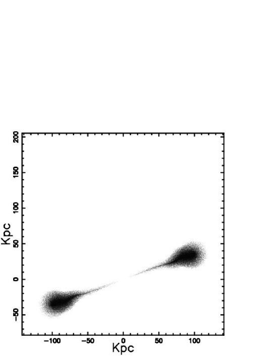
Figure 11: Projected 3D trajectory of CygnusA: the three Eulerian angles (English notation) characterising the point of view are $\Phi$= 90 ^∘ , $\Theta$= 0 ^∘ and $\Psi$=-20 ^∘. The precession is characterised by the angle $\Psi_{prec}$= 1 ^∘ and by the angular velocity $\Omega_{prec}$= 600.00 [${}^{\circ}/10^{7}$ $\mathrm{year}$]. The three Eulerian angles are: $\Phi_{j}$= 0 ^∘ , $\Psi_{j}$= 0 ^∘ and $\Theta_{j}$= 90 ^∘. Parameters of the two–phase continuous model: $x_{0}$= 0.0 ${\mathrm{kpc}}$, $r_{0}$= 0.02 ${\mathrm{kpc}}$, $\beta_{0}$= 0.8 , $t_{2}$= 0.6 $10^{7}$ $\mathrm{year}$, $t_{1}$= 0.161 $10^{7}$ $\mathrm{year}$, $\alpha_{0}$ = 5 ^∘  and  $\alpha_{1}$= 35 ^∘.

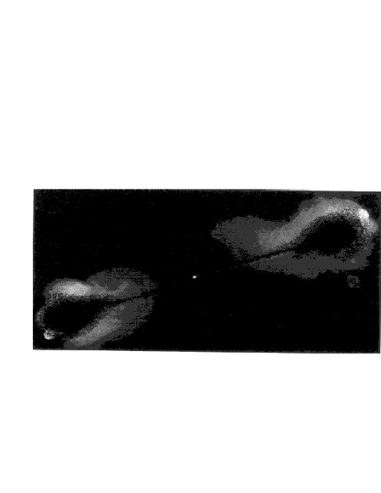
Figure 12: Cygnus from the NRAO Image Gallery (white) superimposed on the theoretical trajectory represented by Figure 11 (black).

Table 10: The physical parameters output of the simulation on Cygnus A

$$\begin{array}[]{cccccc}\hline\cr\hline\cr\vskip 3.0pt plus 1.0pt minus 1.0pt\cr physical\leavevmode\nobreak\ quantity\backslash index&0&1&2\\ \vskip 3.0pt plus 1.0pt minus 1.0pt\cr\hline\cr\vskip 3.0pt plus 1.0pt minus 1.0pt\cr x\leavevmode\nobreak\ [{\mathrm{kpc}}],distance&0.0&60.01&106.18\\ \vskip 3.0pt plus 1.0pt minus 1.0pt\cr r\leavevmode\nobreak\ [\mathrm{kpc}],radius&0.02&5.25&19.81\\ \vskip 3.0pt plus 1.0pt minus 1.0pt\cr v\leavevmode\nobreak\ [{\mathrm{km/s}}],velocity&240000&24577&6518\\ \vskip 3.0pt plus 1.0pt minus 1.0pt\cr t\leavevmode\nobreak\ [10^{7}\mathrm{year}],time&0&0.161&0.6\\ \vskip 3.0pt plus 1.0pt minus 1.0pt\cr\vskip 3.0pt plus 1.0pt minus 1.0pt\cr\hline\cr\hline\cr\end{array}$$

0.8.2 Classic 0647+693

A radio–map of 0647+693 in the 8.5 GHz band can be found in  Hardcastle & Sakelliou (2004) where two radio–images were traced at the resolution of $0.3\times 0.6$ arcsec and 2 arcsec. The influence of the motion of the host galaxy is evident from the maps and can be visualised in the following way

• A line is traced between the two hot–spots.

• The perpendicular to the previous line that intersects the nucleus is traced. The distance along the perpendicular to the previous line turns out to be $\approx$ 36.8 ${\mathrm{kpc}}$.

From Figure 1 of  Hardcastle & Sakelliou (2004) it is also possible to measure the second opening angle , $\alpha_{1}$ that turns out to be $\approx\leavevmode\nobreak\ 25^{\circ}\leavevmode\nobreak\$.

The results of the simulation (as outlined in Section 0.4) are reported in Figure 13(red points) and in Figure 14, with the radio map superimposed on the simulation ; Table 11 reports the data.

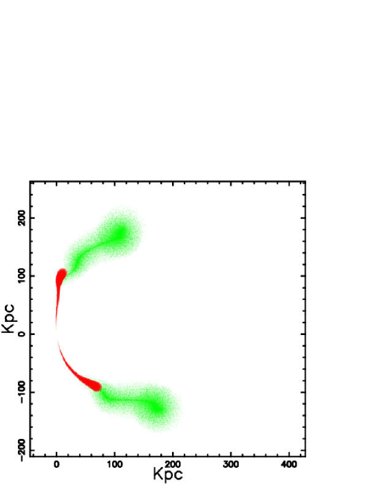
Figure 13: Projected 3D trajectory of 0647+693 (red points): the three Eulerian angles (English notation) characterising the point of view are $\Phi$= 10 ^∘ , $\Theta$= 80 ^∘ and $\Psi$=-10 ^∘. The precession is characterised by the angle $\Psi_{prec}$= 5 ^∘ and by the angular velocity $\Omega_{prec}$= 22.50 [${}^{\circ}/10^{7}\mathrm{year}$]. The three Eulerian angles are: $\Phi_{j}$= 0 ^∘ , $\Psi_{j}$= 0 ^∘ and $\Theta_{j}$= 90 ^∘. Parameters of the two–phase continuous model: $x_{0}$= 0.0001 ${\mathrm{kpc}}$, $r_{0}$= 0.0600 ${\mathrm{kpc}}$, $c_{f}$= 5.0, $t_{2}$= 8.00 $10^{7}\mathrm{year}$, $t_{1}$= 4.00 $10^{7}\mathrm{year}$, $\alpha_{0}$ = 5 ^∘  and  $\alpha_{1}$= 25 ^∘. The green points represents the same trajectory after $t_{2}$= 32.00 $10^{7}{\mathrm{year}}$.

Figure 14: Figure 2 of  Hardcastle & Sakelliou (2004) superimposed on the theoretical trajectory represented by Figure 13(red points).

Table 11: The physical parameters output of the simulation on 0647+693

$$\begin{array}[]{cccccc}\hline\cr\hline\cr\vskip 3.0pt plus 1.0pt minus 1.0pt\cr physical\leavevmode\nobreak\ quantity\backslash position&0&1&2\\ \vskip 3.0pt plus 1.0pt minus 1.0pt\cr\hline\cr\vskip 3.0pt plus 1.0pt minus 1.0pt\cr x\leavevmode\nobreak\ [{\mathrm{kpc}}],distance&0.0001&80.7&104.4\\ \vskip 3.0pt plus 1.0pt minus 1.0pt\cr r\leavevmode\nobreak\ [{\mathrm{kpc}}],radius&0.060&3.6&8.8\\ \vskip 3.0pt plus 1.0pt minus 1.0pt\cr v\leavevmode\nobreak\ [{\mathrm{km/sec}}],velocity&60000.0&1004.7&407.6\\ \vskip 3.0pt plus 1.0pt minus 1.0pt\cr t\leavevmode\nobreak\ [10^{7}\leavevmode\nobreak\ \mathrm{year}],time&0&4.0&8.0\\ \vskip 3.0pt plus 1.0pt minus 1.0pt\cr\vskip 3.0pt plus 1.0pt minus 1.0pt\cr\hline\cr\hline\cr\end{array}$$

In order to reproduce the long trails of 0647+693 visible in Figure 1 of Hardcastle & Sakelliou (2004), the simulation is now performed at a value of $t_{1}$ which is bigger by factor four in respect to the previous run , see Figure 13(green points) and Figure 15, where the radio map is superimposed on the simulation.

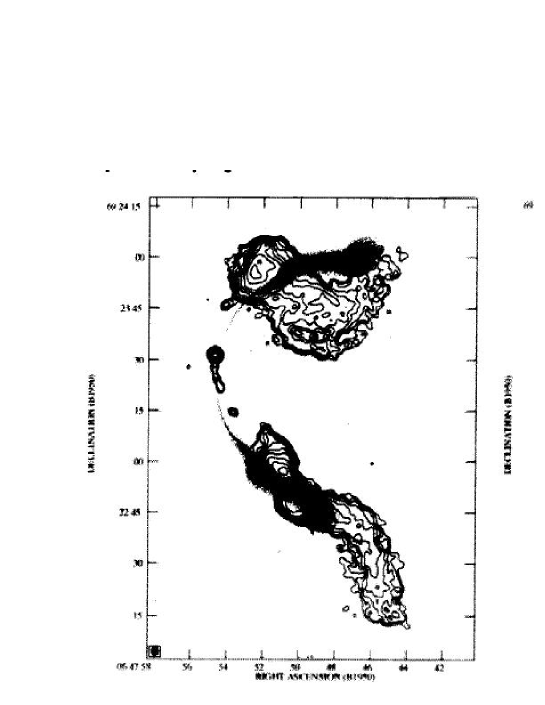
Figure 15: Figure 1 of  Hardcastle & Sakelliou (2004) superimposed on the theoretical trajectory represented by Figure 13(green points).

0.9 The Kelvin-Helmholtz instabilities

The very small opening angles of observed extra-galactic radio–jets , if interpreted as free expansion, in many cases imply a Mach number $M$ $>$ 6 and existing theories are briefly reviewed. Some basic questions can be posed on the stability of such highly supersonic jets :

• Is the jet unstable against perturbation with a wavelength smaller than the radius?

• Is the jet stable over long distances?

• If the jet is unstable, how does the distance over which an instability grows by a factor of e depend upon M and the density contrast between the jet and the external medium?

• Are the helical instabilities with an azimuthal number $m$ = 1 and the pinch instabilities , $m$=0 , enough to build a theory on the lateral growth of the jet due to an increase of energy in the perturbations ?

In order to study these questions, we must analyse the Kelvin-Helmholtz instability of an axisymmetric flow along the $z$-axis when the wavelengths $\lambda=\frac{2\pi}{k}$ ( $k$ is the wave-vector) are smaller or greater than the jet radius $a$, which is taken to be independent of the position along the jet. The velocity , $U_{0}$, is assumed to be rectangular. The internal ( external ) fluid density is represented by $\rho_{0i}$ ($\rho_{0e}$) , the internal sound velocity is $s$ and $\nu_{0}$= $\frac{\rho_{0i}}{\rho_{0e}}$. The analysis is therefore split in two.

0.9.1 Small wavelengths

If the growth rate of the envelope of the reflecting modes is analysed, it is possible to deduce the following approximate relationship for the imaginary ($\gamma_{KH}$) and real ($\omega_{r}$) part of the perturbations when $M\leavevmode\nobreak\ >\leavevmode\nobreak\ 1$

$$\gamma_{KH}=\gamma_{ad}\frac{s}{a}$$ (91)

with

$$\gamma_{ad}\approx 0.17(\ln(kaM))^{1.21}(\frac{2}{\nu_{0}+1/\nu_{0}})^{0.06}(ka)^{0.7}\quad,$$ (92)

and

$$\omega_{r}\approx\frac{M}{2}\nu_{0}^{0.21}ka\frac{s}{a}\quad.$$ (93)

More details can be found in Zaninetti (1986).

0.9.2 Great wavelengths

Starting from the equations of motion and continuity, and assuming both fluids to be adiabatically compressible, it is possible to derive and to solve the dispersion relation numerically , see Zaninetti (1987).

We then start from observable quantities that can be measured on radio-maps such as the total length $L_{obs}$, the wavelength $\lambda_{obs}^{1}$ of the wiggles ($m$=1) along the jet, the distance $\lambda_{obs}^{0}$ ($m$=0) between knots, and the final offset $\Delta\,L_{obs}$ of the center of the jet.

These observable quantities are identified with the following theoretical variables:

$$\lambda^{1}_{max}=\lambda^{1}_{obs}\quad,$$ (94)

$$\lambda^{0}_{max}=\lambda^{0}_{obs}\quad,$$ (95)

$$A_{0}\exp\bigl{(}\frac{2L_{obs}}{Mt_{ad}a})=\Delta L_{obs}\quad,$$ (96)

$$nl_{e}=L_{obs}\quad,$$ (97)

where $t_{ad}$ = $t_{min}\cdot s_{i}/a$ and $A_{0}$ is the amplitude of the perturbed energy. The result is a theoretical expression for $t_{min}$ the minimum time scale of the instability, $\lambda_{max}$ the wavelength connected with the most unstable mode and $l_{e}$ the distance over which the most unstable mode grows by a factor $e$, see  Zaninetti (1987). These parameters can then be found through the set of nonlinear equations previously reported. By choosing three objects, M87 ( Owen et al. (1980)) , NGC6251 (see  Perley et al. (1984a)) and NGC1265 ( see  Odea & Owen (1986)) the observational parameters can be measured on the radio image, see Table 12.

Table 12: Parameters of the observed oscillations in radio–galaxies expressed in averaged radius units

$$\begin{array}[]{lccc}\hline\cr\hline\cr\vskip 3.0pt plus 1.0pt minus 1.0pt\cr Geometrical\leavevmode\nobreak\ misuration&M87&NGC6251&NGC1265\\ \vskip 3.0pt plus 1.0pt minus 1.0pt\cr\hline\cr\vskip 3.0pt plus 1.0pt minus 1.0pt\cr L_{obs}[averaged\leavevmode\nobreak\ radius\leavevmode\nobreak\ units]&48&58.75&20\\ \vskip 3.0pt plus 1.0pt minus 1.0pt\cr\lambda^{0}_{obs}[averaged\leavevmode\nobreak\ radius\leavevmode\nobreak\ units]&4.0&4.89&4\\ \vskip 3.0pt plus 1.0pt minus 1.0pt\cr\lambda^{1}_{obs}[averaged\leavevmode\nobreak\ radius\leavevmode\nobreak\ units]&19.2&17.5&13.3\\ \vskip 3.0pt plus 1.0pt minus 1.0pt\cr\Delta L_{obs}[averaged\leavevmode\nobreak\ radius\leavevmode\nobreak\ units]&0.96&5.87&2\\ \vskip 3.0pt plus 1.0pt minus 1.0pt\cr\vskip 3.0pt plus 1.0pt minus 1.0pt\cr\hline\cr\hline\cr\end{array}$$

The four nonlinear equations are then solved and the four theoretical parameters are found , see Table 13.

Table 13: Theoretical parameters from oscillations deduced from the four nonlinear equations

$$\begin{array}[]{lccc}\hline\cr\hline\cr\vskip 3.0pt plus 1.0pt minus 1.0pt\cr Theoretical\leavevmode\nobreak\ variable&M87&NGC6251&NGC1265\\ \vskip 3.0pt plus 1.0pt minus 1.0pt\cr\hline\cr\vskip 3.0pt plus 1.0pt minus 1.0pt\cr n&2.75&2.88&1.1\\ \vskip 3.0pt plus 1.0pt minus 1.0pt\cr M&17.28&19.44&17.93\\ \vskip 3.0pt plus 1.0pt minus 1.0pt\cr\nu_{0}&9.61&28.05&9.4\\ \vskip 3.0pt plus 1.0pt minus 1.0pt\cr A_{0}&5.57\leavevmode\nobreak\ 10^{-3}&8.2\leavevmode\nobreak\ 10^{-3}&0.25\\ \vskip 3.0pt plus 1.0pt minus 1.0pt\cr\hline\cr\hline\cr\end{array}$$

An application of the results here obtained is reported in Figure 16 where the wavelength of the pinch modes ($m=0$) and the oscillations of the helical mode ($m=1$) as reported in Table 13 are simulated by identifying the lateral growth of energy with the precession. Figure 17 reports the radio map superimposed on the simulation of the pinch modes.

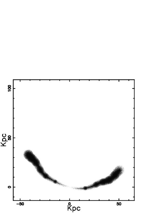
Figure 16: Parameters as in Figure 3, but with superimposition of the pinch mode ($m=0$).

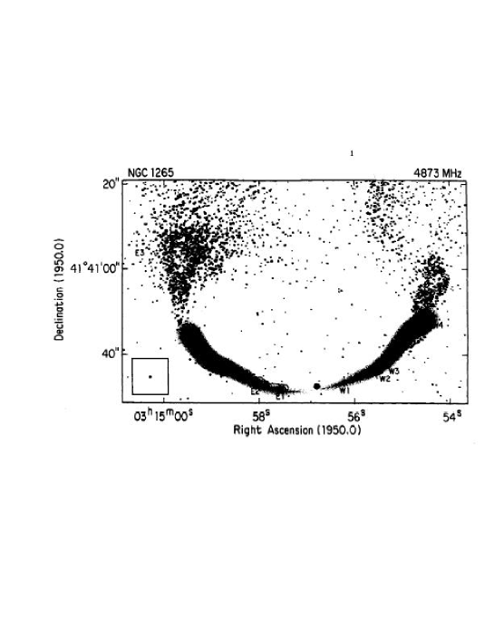
Figure 17: Figure 1 of  Odea & Owen (1986) representing NG1265 at 4873 MHz superimposed on the pinch mode represented by Figure 16.

0.10 Summary

0.10.1 New Physics

The concept of deceleration is both an explanation of observed properties of a sample of radio-galaxies ,see Laing et al. (1999) , as well as an hypothesis of work to explain the deceleration of a relativistic jet of electrons and positron pairs by mass injection, see Laing & Bridle (2002b) , or by adiabatic models that require coupling between the variations of velocity, magnetic field and particle density, see Laing & Bridle (2002b).

Here two new laws of motion for extra-galactic jets in the presence of laminar flow are derived , equation (5) and equation (13), once the two canonical laws of resistance are introduced.

The introduction of the momentum conservation along a solid angle that characterises the extra-galactic jet allows us to find:

• An analytical law ,equation (47), for the velocity and length of the jet as a function of the other structural parameters which are: the involved linear density of energy, the initial radius, the elapsed time and the solid angle. This is the third law of motion.

• An analytical law for the velocity if conversely the conservation of the momentum’s flux in a turbulent jet is assumed, equation (58). This is the fourth law of motion.

• An integral equation (73) of motion if the conservation of the relativistic momentum’s flux in a turbulent jet is assumed. This is the fifth law of motion.

The new equation (20) connects the turbulent eddy viscosity with the jet’s opening angle.

0.10.2 Morphological Results

The introduction of the law of motion allows us to find a space trajectory on introducing the jet precession, the velocity and rotation of the galaxy, and the inclination of the jet with respect to the plane of the galaxy.

It can therefore be suggested that the hydrodynamical effects necessary to bend the jet (see for example Section 4.4.5 of de Young (2002) or the discussion in Odea (1985)) can also be explained as an artifact of a change in the system of reference combined with precession effects of the jet as well as decreasing jet velocity. From an observational point of view it is not easy to discriminate between the bending of the radio-galaxy due to the dynamic pressure , see equation (A35) in de Young (2002) and the bending due to the decreasing jet’s velocity. Both models require a virial speed of the host galaxy $\approx$ 1000${\mathrm{\frac{km}{s}}}$ and differ only in the requirement for the jet’s velocity which is constant in the traditional approach and variable in the models here adopted. This dilemma will be solved when measurements of the jet’s velocity independent from the radio-models will be available. The spectroscopic observations for radio galaxies having ultra steep radio spectra, for example , show velocity shifts range from 100 to almost 1000 $\mathrm{km/s}$ , see Roettgering et al. (1997).

0.10.3 Other approaches

In FR-I jets, which are thought to decelerate, the profile of this deceleration appears in other models that are now briefly reviewed

• In Bowman et al. (1996) a detailed study of the dynamical effects of entraining cool (thermally sub-relativistic) material into hot’ (thermally relativistic) jets is presented. The dissipation associated with entrainment causes only modest loss of kinetic energy flux, and it is shown that relativistic jets are affected much less by dissipation than are classical flows. Their equation (41) represents the flux of kinetic energy but no analytical results are given for the relativistic law of motion such as our formula (73).

• In Laing & Bridle (2002a) the conservation of particles, energy and momentum are applied in order to derive the variations of pressure and density along the jets of the low-luminosity radio galaxy 3C 31. Their self-consistent solutions for deceleration by injection of thermal matter can be compared with our equation (47).

• In Canvin & Laing (2004) some functional forms are introduced to describe the geometry, velocity, emissivity and magnetic-field structure of the two low-luminosity radio galaxies B2 0326+39 and B2 1553+24 and an accurate comparison between models and data is presented. Their solutions are purely numerical and analytical solutions such as our formula (73) are absent.

0.10.4 Analytical results and hydrodynamical codes

A comparison with the hydrodynamical codes is tentatively made on the following key–points

• The hydrodynamical codes are usually performed on a family of parameters given by $M_{b}$ , which is the beam Mach number , while $\rho_{b}$ is the inside/outside density contrast and t is the time over which the phenomena is followed. Due to the fact that the hydrodynamical codes do not give the possibility of closing the equations with parameters deduced from the observations, $\infty$ figures should be produced in order to find the one that better approximates the radiosource chosen to be simulated, see for example Norman (1996) and Balsara & Norman (1992). Conversely, the analytical approach developed here , see eqns. (5),(13), (50) and (51), gives position and velocity once a few input parameters are provided.

• The treatment here adopted can not follow the nonlinear development of the K-H instabilities in 3D , see for example Hardee et al. (1995) where the simulation was performed at $M_{b}$=5; but despite this inconvenience, the concept of developed turbulence with its consequent constant density along the jet is widely used, see Section 0.3 and Section 0.4.

0.10.5 Average density

Here we have assumed that the density of the jet is constant and equal to its surrounding medium. This is certainly something that is not necessarily the case for many astrophysical jets. Some properties can be deduced on the medium surrounding the elliptical galaxies from the X-ray surface brightness distribution. Assuming that the gas is isothermal, the following empirical law ( Fabbiano (1989)) is used for the electron density:

$$n_{e}(r)=n_{e}(0)\left[1+(\frac{r}{ax})^{2}\right]^{-3\beta/2}\quad,$$ (98)

here $\beta$ $\sim$ 0.4 $\div$ 0.6 , $n_{e}(0)$ $\sim$ 0.1 $\mathrm{particles}\over{\mathrm{cm}^{3}}$ and ax $\sim$ 1$\div$ 3${\mathrm{kpc}}$. On adopting this radial dependence for proton density we can evaluate the average density when $n_{e}(0)=0.1\frac{\mathrm{particles}}{\mathrm{cm}^{3}}$, ax = 2.0 ${\mathrm{kpc}}$ and $\beta$= 0.4. The average value of $n_{0}$ , $\overline{n_{0}}$ , when evaluated over 10000 points in the interval 0-100 ${\mathrm{kpc}}$ is $\overline{n_{0}}$ = $6.74\;10^{-3}\frac{\mathrm{particles}}{\mathrm{cm}^{3}}$. This is the theoretical value of $n_{0}$ that should be used , for example , in equation (50).

.11 The roots of a cubic

To solve the cubic polynomial equation

$$a_{{0}}{x}^{3}+a_{{1}}{x}^{2}+a_{{2}}x+a_{{3}}=0\quad,$$ (99)

for $x$, the first step is to apply the transformation

$$x=y-1/3\,{\frac{a_{{1}}}{a_{{0}}}}\quad.$$ (100)

This reduces the equation to

$$y^{3}+py+q=0\quad,$$ (101)

where

$$p = 1/3\,{\frac{3\,a_{{2}}a_{{0}}-{a_{{1}}}^{2}}{{a_{{0}}}^{2}}}$$

$$q = 1/27\,{\frac{27\,a_{{3}}{a_{{0}}}^{2}+2\,{a_{{1}}}^{3}-9\,a_{{2}}a_{{1}}a_{{0}}}{{a_{{0}}}^{3}}}.$$

The next step is to compute the first derivative of the left hand side of equation (101) calling it $f(y)^{\prime}$

$$f(y)^{\prime}=3y^{2}+p\quad.$$ (102)

In the case in which $p\geq 0$ , in the range of existence $-\infty<y<\infty$ , the first derivative is always positive and equation (101) has only one root that is real , more precisely ,

$$y=1/6\,\sqrt[3]{-108\,{\it q}+12\,\sqrt{12\,{{\it p}}^{3}+81\,{{\it q}}^{2}}}-2\,{\frac{{\it p}}{\sqrt[3]{-108\,{\it q}+12\,\sqrt{12\,{{\it p}}^{3}+81\,{{\it q}}^{2}}}}}\quad,$$ (103)

or equation (99) has the solution in terms of $a_{0}$,$a_{1}$,$a_{2}$ and $a_{3}$

$$1/6\,\sqrt[3]{-36\,{\frac{3\,a_{{2}}a_{{0}}-{a_{{1}}}^{2}}{{a_{{0}}}^{2}}}+12\,\sqrt{4/9\,{\frac{\left(3\,a_{{2}}a_{{0}}-{a_{{1}}}^{2}\right)^{3}}{{a_{{0}}}^{6}}}+9\,{\frac{\left(3\,a_{{2}}a_{{0}}-{a_{{1}}}^{2}\right)^{2}}{{a_{{0}}}^{4}}}}}$$

$$-2/3\,\left(3\,a_{{2}}a_{{0}}-{a_{{1}}}^{2}\right){a_{{0}}}^{-2}{\frac{1}{\sqrt[3]{-36\,{\frac{3\,a_{{2}}a_{{0}}-{a_{{1}}}^{2}}{{a_{{0}}}^{2}}}+12\,\sqrt{4/9\,{\frac{\left(3\,a_{{2}}a_{{0}}-{a_{{1}}}^{2}\right)^{3}}{{a_{{0}}}^{6}}}+9\,{\frac{\left(3\,a_{{2}}a_{{0}}-{a_{{1}}}^{2}\right)^{2}}{{a_{{0}}}^{4}}}}}}}.$$ (104)

(105)

References

- Alexander (2000) Alexander, P. 2000, MNRAS , 319, 8
- Balsara & Norman (1992) Balsara, D. S., & Norman, M. L. 1992, ApJ , 393, 631
- Bird et al. (2002) Bird, R., Stewart, W., & Lightfoot, E. 2002, Transport Phenomena ; second Edition (New York: John Wiley and Sons)
- Bliton et al. (1998) Bliton, M., Rizza, E., Burns, J. O., Owen, F. N., & Ledlow, M. J. 1998, MNRAS , 301, 609
- Bowman et al. (1996) Bowman, M., Leahy, J. P., & Komissarov, S. S. 1996, MNRAS , 279, 899
- Burns & Owen (1980) Burns, J. O., & Owen, F. N. 1980, AJ, 85, 204
- Canto & Raga (1996) Canto, J., & Raga, A. C. 1996, MNRAS , 280, 559
- Canvin & Laing (2004) Canvin, J. R., & Laing, R. A. 2004, MNRAS , 350, 1342
- de Young (2002) de Young, D. S. 2002, The physics of extragalactic radio sources (Chicago: University of Chicago Press)
- Fabbiano (1989) Fabbiano, G. 1989, ARA&A, 27, 87
- Fanaroff & Riley (1974) Fanaroff, B. L., & Riley, J. M. 1974, MNRAS , 167, 31P
- Goldstein et al. (2002) Goldstein, H., Poole, C., & Safko, J. 2002, Classical mechanics (San Francisco: Addison-Wesley)
- Goldstein (1965) Goldstein, S. 1965, Modern Developments in Fluid Dynamics (New York: Dover)
- Hardcastle & Sakelliou (2004) Hardcastle, M. J., & Sakelliou, I. 2004, MNRAS , 349, 560
- Hardee et al. (1995) Hardee, P. E., Clarke, D. A., & Howell, D. A. 1995, ApJ , 441, 644
- Hjellming & Johnston (1982) Hjellming, R. M., & Johnston, K. J. 1982, in IAU Symp. 97: Extragalactic Radio Sources, 197–203
- Hughes & Brighton (1967) Hughes, W., & Brighton, J. 1967, Fluid Dynamics (New York: McGraw-Hill)
- Icke & Hughes (1991) Icke, V., & Hughes, P. 1991, Beams and Jets in Astrophysics (Cambridge: Cambridge University Press), 232–+
- Jaffe & Perola (1973) Jaffe, W. J., & Perola, G. C. 1973, A&A , 26, 423
- Kaiser & Alexander (1997) Kaiser, C. R., & Alexander, P. 1997, MNRAS , 286, 215
- Laing & Bridle (2002a) Laing, R. A., & Bridle, A. H. 2002a, MNRAS , 336, 1161
- Laing & Bridle (2002b) —. 2002b, MNRAS , 336, 328
- Laing & Bridle (2004) —. 2004, MNRAS , 348, 1459
- Laing et al. (1999) Laing, R. A., Parma, P., de Ruiter, H. R., & Fanti, R. 1999, MNRAS , 306, 513
- Landau (1987) Landau, L. 1987, Fluid Mechanics 2nd edition (New York: Pergamon Press)
- McCray & Layzer (1987) McCray, R. In: Dalgarno, A., & Layzer, D., eds. 1987, Spectroscopy of astrophysical plasmas
- Mendoza et al. (2005) Mendoza, S., Hernández, X., & Lee, W. H. 2005, Revista Mexicana de Astronomia y Astrofisica, 41, 453
- Mendoza & Longair (2001) Mendoza, S., & Longair, M. S. 2001, MNRAS , 324, 149
- Mendoza & Longair (2002) —. 2002, MNRAS , 331, 323
- Miller et al. (2002) Miller, J. M., Ballantyne, D. R., Fabian, A. C., & Lewin, W. H. G. 2002, MNRAS , 335, 865
- Murgia et al. (2001) Murgia, M., Parma, P., de Ruiter, H. R., Bondi, M., Ekers, R. D., Fanti, R., & Fomalont, E. B. 2001, A&A , 380, 102
- Nakamura et al. (2001) Nakamura, M., Uchida, Y., & Hirose, S. 2001, New Astronomy, 6, 61
- Norman (1996) Norman, M. L. 1996, in ASP Conf. Ser. 100: Energy Transport in Radio Galaxies and Quasars, 405–+
- Norman et al. (1994) Norman, M. L., Balsara, D., & O’Dea, C. 1994, Bulletin of the American Astronomical Society, 26, 879
- Odea (1985) Odea, C. P. 1985, ApJ , 295, 80
- Odea & Owen (1986) Odea, C. P., & Owen, F. N. 1986, ApJ , 301, 841
- Owen et al. (1980) Owen, F. N., Hardee, P. E., & Bignell, R. C. 1980, ApJ , 239, L11
- Perley et al. (1984a) Perley, R. A., Bridle, A. H., & Willis, A. G. 1984a, ApJS, 54, 291
- Perley et al. (1984b) Perley, R. A., Dreher, J. W., & Cowan, J. J. 1984b, ApJ , 285, L35
- Raga & Canto (1996) Raga, A. C., & Canto, J. 1996, MNRAS , 280, 567
- Reichardt (1942) Reichardt, V. 1942, VDI-Forschungsheft, 414, 141
- Reichardt (1951) —. 1951, Z.angew, Math. Mech., Bd., 31
- Roettgering et al. (1997) Roettgering, H. J. A., van Ojik, R., Miley, G. K., Chambers, K. C., van Breugel, W. J. M., & de Koff, S. 1997, A&A , 326, 505
- Schlichting (1979) Schlichting, H. 1979, Boundary Layer Theory (New York: McGraw-Hill)
- Sedov (1959) Sedov, L. I. 1959, Similarity and Dimensional Methods in Mechanics (New York: Academic Press)
- Valtonen & Kotilainen (1989) Valtonen, M. J., & Kotilainen, J. 1989, AJ, 98, 117
- Venkatesan et al. (1994) Venkatesan, T. C. A., Batuski, D. J., Hanisch, R. J., & Burns, J. O. 1994, ApJ , 436, 67
- Zaninetti (1986) Zaninetti, L. 1986, Physics of Fluids, 29, 332
- Zaninetti (1987) —. 1987, Physics of Fluids, 30, 612
- Zaninetti (1989) —. 1989, A&A , 221, 204