Primordial Non-Gaussianity and Gravitational Waves: Observational Tests of Brane Inflation in String Theory

Abstract

We study brane inflation scenarios in a warped throat geometry and show that there exists a consistency condition between the non-Gaussianity of the curvature perturbation and the amplitude and scale-dependence of the primordial gravitational waves. This condition is independent of the warping of the throat and the form of the inflaton potential. We find that such a relation could be tested by a future CMB polarization experiment if the Planck satellite is able to detect both a gravitational wave background and a non-Gaussian statistic. In models where the observable stage of inflation occurs when the brane is in the tip region of the throat, we derive a further consistency condition involving the scalar spectral index, the tensor-scalar ratio and the curvature perturbation bispectrum. We show that when such a relation is combined with the WMAP3 results, it leads to a model-independent bound on the gravitational wave amplitude given by $10^{-3}<r<10^{-2}$. This corresponds to the range of sensitivity of the next generation of CMB polarization experiments.

I Introduction

The inflationary scenario, whereby the universe underwent a phase of accelerated expansion in its most distant past, represents the cornerstone of modern, early universe cosmology simplest ; perturbations . It has proved remarkably successful when confronted with cosmological observations, in particular the three-year data from the Wilkinson Microwave Anisotropy Probe (WMAP3) spergel . String theory is presently the favoured candidate for a unified theory of the fundamental interactions including gravity and it is therefore important to embed inflation within string theory.

One approach to string-theoretic inflation is based on ${\rm D}$-branes earlybrane ; kklt ; kklmmt ; silverstein ; chensolo ; shandtye ; tipinflation ; otherbranes . Of particular interest are scenarios where a type IIB orientifold is compactified on a Calabi-Yau (CY) three-fold, where the moduli fields are stabilized due to the presence of non-trivial flux gkp ; kklt . (See fluxcompact for a review). These fluxes generate local regions within the CY space with a warped geometry or ‘throat’. In many settings, an anti-${\rm D3}$-brane sits naturally at the infra-red (IR) tip of the throat and attracts a ${\rm D3}$-brane towards it. The brane separation then plays the role of the inflaton and, since this is an open string mode, its dynamics is determined by a Dirac-Born-Infeld (DBI) action. In general, there are two limiting regimes for brane inflation which are characterized by the rolling of the inflaton. In the KKLMMT scenario, for example, the inflaton undergoes conventional slow-roll down a flat potential kklmmt . However, the non-linear nature of the DBI action implies that inflation may also proceed when the field is rolling relatively fast, as is the case in DBI inflation silverstein ; chensolo ; shandtye .

In this paper, we investigate how the brane inflationary scenario could be tested if forthcoming observations of the Cosmic Microwave Background (CMB) uncover non-Gaussian statistics in the scalar (density) perturbation spectrum and also a primordial background of tensor (gravitational wave) perturbations. An observed departure from purely Gaussian statistics will provide a powerful discriminant between different inflationary models and the Planck satellite, which is scheduled for launch in 2007, will improve on the WMAP3 sensitivity by an order of magnitude planck . On the other hand, the detection of gravitational waves will open up a direct window onto the energy scale of inflation. The most promising means of detecting tensor perturbations is through the $B$-mode polarization of the CMB and a number of experiments, such as Clover (the ‘Cl-Observer’) clover , are presently under construction. (For a review, see, e.g., cmbreview ).

The paper is organized as follows. We begin by summarizing the brane inflation scenario in Section 2. In Section 3, we derive a consistency condition between the non-Gaussianity of the curvature perturbation and the amplitude and scale-dependence of the gravitational waves. This relation is independent of the warped geometry and the inflaton potential. We then discuss the prospects for testing such a condition with future CMB polarization experiments. In Section 4, we consider the class of models where the observable phase of inflation occurred when the ${\rm D}$-brane was near the IR tip of the throat. We derive a further consistency condition in this regime that relates the scalar spectral index, the tensor-scalar ratio and the bispectrum of the curvature perturbation. We find that such a constraint leads to a bound on the gravitational wave amplitude of $10^{-3}<r<10^{-2}$, which is in the range of sensitivity of the next generation of CMB polarization experiments. We conclude with a discussion in Section 6.

II Brane Inflation in String Theory

In general, the low energy world-volume dynamics of a probe ${\rm D3}$-brane in a warped background is given by

$$S=\int d^{4}x\sqrt{|g|}\left[\frac{m_{\rm pl}^{2}}{16\pi}R+P(\phi,X)\right]$$ (1)

$$P(\phi,X)=f_{1}(\phi)\sqrt{1+f_{2}(\phi)X}-f_{3}(\phi),$$ (2)

where $R$ is the Ricci curvature scalar, $X\equiv-\frac{1}{2}g^{\mu\nu}\nabla_{\mu}\phi\nabla_{\nu}\phi$ is the kinetic energy of the inflaton field, $\phi$, and the functions $f_{i}(\phi)$ are determined by the warped geometry and the inflaton self-interaction potential.

A concrete example of a warped background is the Klebanov-Strassler (KS) solution of the type IIB theory, where the throat is a warped deformed conifold ks . The ten-dimensional metric has the form $ds_{10}^{2}=\tilde{f}^{-1/2}(\tau)\eta_{\mu\nu}dx^{\mu}dx^{\nu}+\tilde{f}^{1/2}(\tau)ds_{6}^{2}$, where $\tilde{f}(\tau)$ denotes the warp factor and $\tau$ is the coordinate along the throat (corresponding to one of the coordinates on $ds_{6}^{2}$). In the ultra-violet (UV) regime ($\tau\rightarrow\infty$) the throat corresponds to a cone over the Einstein manifold $T^{1,1}={\rm SU(2)}\otimes{\rm SU(2)}/{\rm U(1)}$, which has a topology $S^{2}\times S^{3}$, where the $S^{2}$ is fibred over the $S^{3}$. On the other hand, at the tip of the throat ($\tau\rightarrow 0$) the wrapping of the fluxes along the cycles of the conifold smooths out the conical singularity with an $S^{3}$ ‘cap’ ks ; kt .

The effective DBI action for a ${\rm D}$-brane in this background is given by tipinflation

$$P=-T_{3}\left[\frac{1}{\tilde{f}(\tau)}\left(\sqrt{1+h(\tau)(\nabla\tau)^{2}}-1\right)+V(\tau)\right],$$ (3)

where the warp factor is

$$\tilde{f}(\tau)=AI(\tau),\qquad h(\tau)=B\frac{I(\tau)}{K^{2}(\tau)}$$ (4)

$$I(\tau)=\int_{\tau}^{\infty}dx\,\frac{x\,{\rm coth}(x)-1}{\sinh^{2}(x)}\left[\sinh(2x)-2x\right]^{1/3}$$ (5)

$$K(\tau)=\frac{[\sinh(2\tau)-2\tau]^{1/3}}{2^{1/3}\sinh(\tau)}.$$ (6)

The brane tension is denoted by $T_{3}$, $V(\tau)$ is a non-perturbative potential and $\{A,B\}$ are model-dependent constants.

Since the aim of this paper is to identify model-independent, observational tests of brane inflation that are insensitive to the specific form of the inflaton potential and the nature of the warped geometry, we will assume that the form of the kinetic function $P(\phi,X)$ is given by Eq. (2) for arbitrary $f_{i}(\phi)$, subject only to the condition that a successful phase of inflation can be realised. We will exploit the fact that the non-trivial kinetic structure in $P(\phi,X)$ causes the sound speed of fluctuations in the inflaton to differ from unity (the value it takes in canonical, single-field inflation, where $P=X-V(\phi)$). This will lead to observational signatures involving both non-Gaussianity and gravitational waves.

The Friedmann equations derived from action (1) take the form

$$3m_{\rm pl}^{2}H^{2}=8\pi E,\qquad\dot{E}=-3H(E+P),$$ (7)

where $E=2XP_{,X}-P$, $H$ represents the Hubble parameter, a dot denotes $d/dt$ and a comma denotes a partial derivative. The inflationary dynamics for this class of models can be quantified in terms of three ‘slow-roll’ parameters:

$$\epsilon\equiv-\frac{\dot{H}}{H^{2}},\qquad\eta\equiv\frac{\dot{\epsilon}}{\epsilon H},\quad s\equiv\frac{\dot{c}_{s}}{c_{s}H},$$ (8)

where

$$c_{s}^{2}\equiv\frac{P_{,X}}{P_{,X}+2XP_{,XX}}$$ (9)

defines the sound speed, $c_{s}$. The rate of change of the sound speed is determined by $s$ and we will assume throughout that $\{\epsilon,|\eta|,|s|\}\ll 1$ during the observable phase of inflation.

The amplitudes of the scalar and tensor perturbation spectra are given by

$$P_{S}^{2}=\frac{1}{\pi m_{\rm pl}^{2}}\frac{H^{2}}{c_{s}\epsilon},\qquad P_{T}^{2}=\frac{16}{\pi}\frac{H^{2}}{m_{\rm pl}^{2}},$$ (10)

respectively, and the corresponding spectral indices are gm

$$1-n_{s}=2\epsilon+\eta+s,\qquad n_{t}=-2\epsilon.$$ (11)

The tensor-scalar ratio, $r\equiv P_{T}^{2}/P_{S}^{2}$, is directly related to the tensorial spectral index such that gm

$$r=-8c_{s}n_{t}.$$ (12)

Finally, deviations from purely Gaussian statistics arise when the primordial three-point function for the curvature perturbation is non-trivial. It is conventional to write the non-Gaussian curvature perturbation ${\cal{R}}$ as a sum of a Gaussian part and the square of a Gaussian such that ${\cal{R}}={\cal{R}}_{G}+f_{NL}({\cal{R}}^{2}_{G}-\langle{\cal{R}}^{2}_{G}\rangle)$, where the quadratic part is a convolution and $f_{NL}$ defines the ‘non-linearity’ parameter maldacena . In general, this parameter is a function of the three momenta which form a triangle in Fourier space. Recently, it was shown that in the equilateral triangle limit (where the three momenta have equal magnitude), the leading-order contribution to the non-linearity parameter is given by chen

$$f_{NL}=\frac{35}{108}\left(\frac{1}{c_{s}^{2}}-1\right)-\frac{5}{81}\left(\frac{1}{c_{s}^{2}}-1-2\Lambda\right),$$ (13)

where

$$\Lambda\equiv\frac{X^{2}P_{,XX}+\frac{2}{3}X^{3}P_{,XXX}}{XP_{,X}+2X^{2}P_{,XX}}.$$ (14)

The bound on the non-linearity parameter imposed by WMAP3 is $|f_{NL}|\lesssim 300$ spergel ; crim .

III An Observational Test of Brane Inflation

It was observed in chen ; tipinflation that when $f_{1}=1/f_{2}$, the second term on the right-hand side of Eq. (13) vanishes, i.e.,

$$\Lambda=\frac{1}{2}\left(\frac{1}{c_{s}^{2}}-1\right).$$ (15)

It can be further shown that for arbitrary $f_{i}(\phi)$, Eq. (2) is the most general form of the kinetic function $P(\phi,X)$ which satisfies Eq. (15). Specifically, we may employ the definitions (9) and (14) to express Eq. (15) in the form of a third-order, non-linear partial differential equation:

$$P_{,X}P_{,XXX}=3P^{2}_{,XX}.$$ (16)

However, Eq. (16) can be reduced to the first-order equation

$$Z_{,X}=2Z^{2}$$ (17)

by defining a new variable $Z\equiv P_{,XX}/P_{,X}$. This admits the general solution $Z(\phi,X)=[f(\phi)-2X]^{-1}$, where $f(\phi)$ is an arbitrary function. Integrating this solution twice then yields the general solution for $P(\phi,X)$, which is precisely the form given in Eq. (2), where the $f_{i}(\phi)$ arise as arbitrary integration functions.

It follows, therefore, that for the general class of string-theoretic models (2), the leading-order contribution to the non-linearity parameter is determined entirely by the sound speed:

$$f_{NL}=\frac{1}{3}\left(\frac{1}{c_{s}^{2}}-1\right).$$ (18)

This implies that we may substitute Eq. (18) into Eq. (12) to deduce a ‘consistency’ equation which is composed entirely of observable parameters:

$$r+8n_{t}=-r_{l}r$$ (19)

$$r_{l}\equiv\sqrt{1+3f_{NL}}-1.$$ (20)

Eq. (19) is model-independent in the sense that it holds for an arbitrary inflaton potential and a general warping of the higher-dimensional spacetime. This is important since the precise form of the potential depends on non-perturbative features of the superpotential, whereas the warp factor is determined by the details of the flux compactification. We may therefore regard Eq. (19) as a robust prediction for string-theoretic brane inflation and it is natural to investigate whether it could be employed as a future test of the scenario. Since it formally reduces to the standard consistency equation of slow-roll inflation in the limit $r_{l}\rightarrow 0$, a detection of Eq. (19) would amount to detecting a violation of the standard consistency equation. A necessary condition for such a detection is that the magnitude of the right-hand side of Eq. (19) should exceed the experimental error in the quantity on the left-hand side SK ; LS . Recently, Song and Knox SK have considered the level of accuracy that should be attainable with future all-sky CMB polarization experiments with angular resolutions in the range $1.0^{\prime}\leq\varphi\leq 30.0^{\prime}$ and noise levels between $1\mu{\rm K}\cdot{\rm arcmin}\leq\Delta\leq 15\mu{\rm K}\cdot{\rm arcmin}$. They determined the anticipated error in $r+8n_{t}$ as a function of the tensor-scalar ratio and this is shown in Fig. 1. The straight lines in this figure correspond to the right-hand side of Eq. (19). For a given value of the non-linearity parameter $f_{NL}$, the point of intersection between the solid and dashed lines yields the minimal value of $r$ above which a detection of Eq. (19) will be possible in principle. This bound is illustrated in Fig. 2.

Figure 1: The dashed line illustrates the results of Song and Knox SK anticipating the experimental error, $\sigma$, in $r+8n_{t}$ as a function of $r$ for a future all-sky CMB polarization experiment with angular resolution $\varphi=3^{\prime}$ and noise $\Delta=3\mu{\rm K}\cdot{\rm arcmin}$ SK . The modulus of the right-hand side of the consistency equation (19) is represented by a straight line for a given value of the non-linearity parameter, $f_{NL}$. The point of intersection of the lines yields a lower bound on the tensor-scalar ratio for a detection of the consistency equation (19) to be possible.

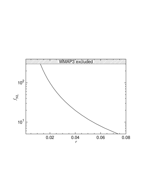
Figure 2: Illustrating the minimal value of the non-linearity parameter $f_{NL}$ deduced from Fig. 1 that will lead in principle to a detection of the consistency equation (19). For a given fiducial value of the tensor-to-scalar ratio, $r$, a detection should be possible in the region of parameter space above the solid line. The shaded region is excluded by the WMAP3 data.

It is interesting to consider what could be deduced from the Planck satellite about our prospects for detecting Eq. (19) with a future CMB polarization experiment. Planck will have sensitivities down to $r\approx 0.05$ and $f_{NL}\approx 5$ planck ; komatsu . For $r=0.05$, one would require $f_{NL}>12$ for a detection of Eq. (19). This is comfortably below the upper limit of $f_{NL}\lesssim 300$ imposed by the WMAP3 data spergel . On the other hand, for $f_{NL}\approx 5$, a detection will only be possible if $r>0.07$. Moreover, imposing the WMAP3 limit $f_{NL}\simeq 300$ implies a future detection would require $r>0.01$, but a value $r\approx 0.01$ should be detectable by Clover at approximately the $3$-sigma level clover . Consequently, future all-sky observations will fail to detect Eq. (19) if Clover does not detect a primordial tensor spectrum. On the other hand, if Planck measures both $r$ and $f_{NL}$, the prospects for the detection of Eq. (19) are good.

IV Brane Inflation Near the Tip

Thus far, our discussion has been general, in the sense that the functions $f_{i}(\phi)$ in action (2) have remained unspecified. In this section, we focus on the case where the ${\rm D}$-brane is in the vicinity of the IR tip of the warped throat. To date, the majority of studies into DBI inflation have considered the dynamics of the brane when it is far from the tip and in a region where the throat is asymptotically ${\rm AdS}_{5}$ silverstein ; chensolo ; shandtye . However, in the UV version of DBI inflation, the brane moves into the throat and reheating occurs when it reaches the tip. Since the era of inflation that is accessible to observations occurred during the last 30-60 e-folds, the brane may well have been near the tip of the throat during that epoch.

DBI inflation in the tip region of the KS background was considered recently in Ref. tipinflation . Near the tip, $\tau\rightarrow 0$, and it can be shown that $I(\tau\rightarrow 0)\rightarrow 0.7$ and $K(\tau\rightarrow 0)\rightarrow(2/3)^{1/3}$. Consequently, the warp factors in Eq. (4) both tend to finite constants in this limit ks .

Motivated by the above asymptotic behaviour of the KS throat, we consider the class of models (2), where $(f_{1},f_{2})\rightarrow{\rm constants}$. On the other hand, we will keep the inflaton potential $f_{3}(\phi)$ arbitrary (modulo the usual caveats for successful inflation). Since $P_{,X\phi}=0$ in this case, it follows after differentiating Eq. (9) with respect to time and using the Friedmann equation (7) that SL1

$$\Lambda=\frac{2(1+c_{s}^{2})s+(1-c_{s}^{2})(2\epsilon-\eta)}{6c_{s}^{2}(2\epsilon-\eta)}.$$ (21)

Combining Eqs. (15) and (21) therefore leads to a constraint equation that relates the sound speed directly to the three slow-roll parameters $\{\epsilon,\eta,s\}$:

$$\frac{1+c_{s}^{2}}{1-c_{s}^{2}}=\frac{2\epsilon-\eta}{s}.$$ (22)

Eq. (22) may be converted into a consistency relation if four observable parameters involving $\{\epsilon,\eta,c_{s},s\}$ can be identified. Eqs. (11) and (18) provide three of these in the form of the two spectral indices and the non-linearity parameter, $f_{NL}$. A possible candidate for the fourth parameter is the running of the tensor spectral index, which is defined by $\alpha_{t}\equiv dn_{t}/d\ln k\approx n_{t}\eta$, where $k$ is the comoving wavenumber. It then follows after some algebra that Eq. (22) is equivalent to

$$\left(\frac{2+3f_{NL}}{1+3f_{NL}}\right)(1-n_{s})=-2n_{t}+\frac{2}{1+3f_{NL}}\frac{\alpha_{t}}{n_{t}}.$$ (23)

On the other hand, we may also define a ‘spectral index’ for the non-linearity parameter, $n_{NL}\equiv d\ln f_{NL}/d\ln k$ chenrunning . In this case, it follows that

$$s=-\frac{3}{2}\left(\frac{f_{NL}}{1+3f_{NL}}\right)n_{NL}$$ (24)

and substituting Eqs. (11), (18) and (24) into Eq. (22) then implies that

$$1-n_{s}=-2n_{t}+\frac{n_{NL}}{1+3f_{NL}}.$$ (25)

Although Eqs. (23) and (25) directly relate observable parameters, it is not clear whether future observations will be able to measure $\alpha_{t}$ or $n_{NL}$ to sufficient accuracy for either of these expressions to be tested. Nonetheless, the form of these constraints is such that the terms involving $\alpha_{t}$ and $n_{NL}$ rapidly become negligible when $f_{NL}\gg 1$. Indeed, for a detectable non-Gaussianity of $f_{NL}>5$, a good approximation to either Eq. (23) or Eq. (25) is

$$1-n_{s}\simeq-2n_{t}.$$ (26)

Moreover, the consistency equation (19) may be employed to express this constraint in terms of the observable parameters $\{n_{s},r,f_{NL}\}$:

$$1-n_{s}\simeq 0.4r\sqrt{f_{NL}}.$$ (27)

Eq. (27) may be interpreted as a new consistency equation for brane inflation which is valid when the level of non-Gaussianity is sufficiently large and when the warp factor of the throat is approximately constant.

A number of results may be deduced from Eq. (27). Firstly, it predicts a red density perturbation spectrum $(n_{s}<1)$ for an arbitrary inflaton potential. Such a spectrum is favoured by the WMAP3 data spergel . Secondly, since the observed deviations from a scale-invariant spectrum are small, it also predicts that a large non-Gaussian contribution to the curvature perturbation will be accompanied by a small tensor-scalar ratio, and vice-versa. As a result, we should not expect to simultaneously observe both a sizeable non-Gaussian signal and a gravitational wave background in these models. On the other hand, if a departure from pure scale-invariance is confirmed, the present-day upper limit on $f_{NL}$ will impose a lower limit on $r$, and vice-versa.

In view of this, let us consider what can be deduced from present-day observational limits. If a power-law spectrum is assumed, the WMAP3 data implies that spergel

$$n_{s}=0.987^{+0.019}_{-0.037}$$ (28)

when the tensor-scalar ratio is included as a free parameter. Substituting the upper bound $1-n_{s}<0.05$ into Eq. (27) then yields the limit

$$r<\frac{1}{8\sqrt{f_{NL}}}.$$ (29)

Alternatively, imposing the WMAP3 upper bound $f_{NL}\simeq 300$ implies that

$$r>\frac{1-n_{s}}{7}.$$ (30)

Thus, for given values of $\{n_{s},f_{NL}\}$, the tensor-scalar ratio is bounded from above and below. This has a number of important implications. In Fig. 3, the solid and dot-dashed lines represent Eq. (27) when the spectral index takes the WMAP3 lower limit $(n_{s}=0.95)$ and central value $(n_{s}=0.987)$, respectively. For a given measurement of $f_{NL}$, the allowed values of $r$ fall below the solid line. We conclude, therefore, that if Planck detects a non-Gaussian signal ($f_{NL}\gtrsim 5$), the tensor-scalar ratio is predicted to lie below $r\lesssim 0.05$, which is close to the optimal sensitivity of Planck. This suggests that a simultaneous detection of both non-Gaussianity and gravitational waves by Planck will not be possible for these brane inflation scenarios. Consequently, a detection of both effects would rule out such models.

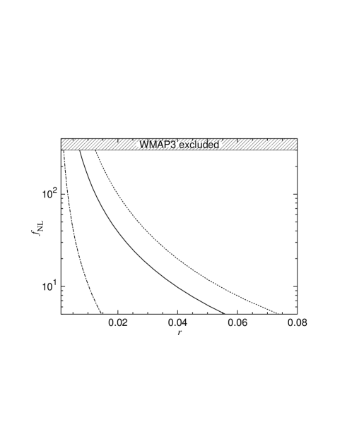
Figure 3: Illustrating the constraint equation (27) for the WMAP3 best-fit value $n_{s}=0.987$ (dot-dashed line) and lower limit $n_{s}=0.95$ (solid line). The region of parameter space consistent with WMAP3 lies below the solid line. The dashed line represents the curve from Fig. 2, above which the general consistency condition (19) will be detectable.

On the other hand, Eq. (27) is such that the departure away from scale-invariance is determined by the combination $r\sqrt{f_{NL}}$. This implies that for fixed values of the non-linearity parameter in the range $5<f_{NL}<300$, the allowed range of $r$ becomes progressively narrower as $n_{s}\rightarrow 1$. For example, the relative steepness of the dot-dashed line in Fig. 3 implies that if (as expected) the spectral index is ultimately measured to a very high accuracy, a confirmed detection of the non-linearity parameter (regardless of the error in the measurement) will strongly constrain the tensor-scalar ratio . Indeed, for the WMAP3 central value $n_{s}=0.987$, the tensor-scalar ratio is bounded by $0.002<r<0.015$. The existence of such a lower limit on $r$ is of particular interest given that future space-based CMB polarization experiments with current detector technology and full sky coverage should be able to detect $r\approx 10^{-3}$ at the $3$-sigma level SK ; vpj .

Finally, we have also superimposed Fig. 1 as the dashed line in Fig. 2. The general consistency equation (19) will only be observable with future all-sky CMB experiments in the region above this line and, since it lies in the region of parameter space that is inconsistent with the WMAP3 upper limit (29), a detection of primordial non-Gaussianity by Planck will immediately imply that the tensor-scalar ratio will be too small for the consistency equation (19) to be detectable. Consequently, an observed violation of the standard consistency equation would rule out this class of models.

V Discussion

There exist many compactification solutions in string theory and it is therefore important to identify observational constraints and tests of string-theoretic inflation that are insensitive to our universe’s location in the string landscape. In this paper, we have considered this question within the context of possible non-Gaussian and gravitational wave signatures from brane inflationary scenarios, both for an arbitrary warp factor and for the case where the warp factor is approximately constant. Furthermore, the form of the inflaton potential has remained unspecified throughout. The constraints we have discussed are also independent of whether the brane is moving into or out of the throat and therefore apply to both the UV and IR versions of DBI inflation silverstein ; chensolo ; shandtye ; tipinflation . However, we have only considered radial motion of the brane in the throat, and have ignored fluctuations of the brane in its internal angular directions. As was emphasized recently lythriotto , such fluctuations may generate a significant contribution to the curvature perturbation.

In general, the standard inflationary consistency equation is violated in brane inflation. The magnitude of the correction depends on the non-linearity parameter, $f_{NL}$. Consequently, the level of non-Gaussianity determines whether or not such a violation will be detectable in future CMB polarization experiments. We find that if Planck detects a gravitational wave background and measures $f_{NL}>10$, a future all-sky CMB polarization satellite should be sufficiently accurate to detect (or rule out) the consistency condition (19). Similarly, this equation should be testable if Planck detects a non-Gaussian signal ($f_{NL}>5$) and Clover measures the tensor-scalar ratio $(r>0.01)$. On the other hand, no departure from the standard consistency equation will be detectable if Clover fails to detect gravitational waves ($r<0.01$).

We have identified a new consistency condition, Eq. (27), which involves the set of observables $\{n_{s},r,f_{NL}\}$. This equation applies in the limit where the warp factor of the throat is approximately constant, which is the case for the KS background in the region near to the tip of the throat. This is a potentially strong constraint, since it allows general conclusions to be drawn for this class of models. In particular, it predicts a red scalar perturbation spectrum, $n_{s}<1$.

Eq. (27) also provides insight into why it has proved difficult to construct brane inflation models with both a high tensor-scalar ratio and a large non-Gaussian contribution to the curvature perturbation shandtye ; tipinflation . Indeed, the bound (30) implies that any model which predicts a very low gravitational wave amplitude ($r<10^{-3}$) will generate a non-Gaussianity in excess of the WMAP3 limit unless the spectral index is extremely close to unity. Consequently, the constraint (30) may be employed to rule out specific models without needing to explicitly calculate the level of non-Gaussianity.

As an example, let us consider the scenario discussed recently by Panda et al. panda , where inflation is generated by the radial motion of a probe BPS ${\rm D}3$-brane in the presence of a stack of coincident and static BPS ${\rm D5}$-branes. The effective DBI action for the ${\rm D3}$-brane is given by Eq. (2) with $f_{2}(\phi)=2$ and $f_{3}=0$ kutasov . In this model, the warp factor $f_{1}(\phi)\rightarrow 1$ as $\phi\rightarrow\infty$ and it can be shown that in this limit the spectral index and tensor-scalar ratio are given by

$$1-n_{s}=\frac{3}{2N_{e}},\qquad r=\frac{\sqrt{\sigma}}{N^{3/2}_{e}},$$ (31)

respectively, where $N_{e}$ is the number of e-folds before the end of inflation and $\sigma\ll 1$ is a parameter that depends on the number of ${\rm D5}$-branes that are present panda . The constraint (30) then implies that the WMAP3 non-Gaussianity limit is only satisfied if $N_{e}<22\sigma$, but even for $\sigma=1$ this would require $(1-n_{s})>0.07$, which is marginally inconsistent with observations. Hence, inflation in this region of parameter space is probably ruled out.

Finally, Eq. (27) implies a lower limit on the tensor-scalar ratio for a given value of the spectral index. In general, we expect $(1-n_{s})$ to be of the order a few percent since typically $1-n_{s}\approx 1/N_{e}$, where $30<N_{e}<60$. In this case, a detection of non-Gaussianity by Planck would imply that $r>10^{-3}$, which will be accessible to the next generation of CMB polarization experiments SK ; vpj . This is interesting since the potential benefits of building such an experiment have been questioned recently given the dearth of well-motivated models which predict $10^{-3}<r<10^{-2}$ desert . Our results therefore provide strong motivation for developing specific brane inflation models based on more general throat geometries and compactification schemes.

References

- (1) A. A. Starobinsky, Phys. Lett. B 91, 99 (1980); A. H. Guth, Phys. Rev. D. 23, 347 (1981); A. Albrecht and P. J. Steinhardt, Phys. Rev. Lett. 48, 1220 (1982); S. W. Hawking and I. G. Moss, Phys. Lett. B 110, 35 (1982); A. D. Linde, Phys. Lett. B 108, 389 (1982); A. D. Linde, Phys. Lett. B 129, 177 (1983).
- (2) V. Mukhanov and G. Chibisov, Pis’ma Zh. Eksp. Teor. Fiz. 33, 549 (1981) [JETP Lett. 33, 532 (1981), arXiv:astro-ph/0303077]; A. H. Guth and S. Y. Pi, Phys. Rev. Lett. 49, 1110 (1982); S. W. Hawking, Phys. Lett. B 115, 295 (1982); A. A. Starobinsky, Phys. Lett. B 117, 175 (1982); A. D. Linde, Phys. Lett. B 116, 335 (1982); J. M. Bardeen, P. J. Steinhardt and M. S. Turner, Phys. Rev. D 28, 679 (1983).
- (3) D. N. Spergel, et al., arXiv:astro-ph/0603449.
- (4) G. R. Dvali and S-H. Tye, Phys. Lett. B 450, 72 (1999), arXiv:hep-ph/9812483; G. R. Dvali, Q. Shafi and S. Solganik, arXiv:hep-th/0105203; C. P. Burgess, M. Majumdar, D. Nolte, F. Quevedo, G. Rajesh, and R. J. Zhang, JHEP 0107, 047 (2001), arXix:hep-th/0105204.
- (5) S. Kachru, R. Kallosh, A. Linde, and S. P. Trevedi, Phys. Rev. D 68, 046005 (2003), arXiv:hep-th/0301240.
- (6) S. Kachru, R. Kallosh, A. Linde, J. Maldacena, L. McAlister, and S. P. Trevedi, JCAP 0310, 013 (2003), arXiv:hep-th/0308055.
- (7) E. Silverstein and D. Tong, Phys. Rev. D 70, 103505 (2004), arXiv:hep-th/0310221; M. Alishahiha, E. Silverstein and D. Tong, Phys. Rev. D 70, 123505 (2004), arXiv:hep-th/0404084.
- (8) X. Chen, Phys. Rev. D 71, 063506 (2005), arXiv:hep-th/0408084; X. Chen, JHEP 0508, 045 (2005), arXiv:hep-th/0501184.
- (9) S. E. Shandera and S-H. Tye, JCAP 0605, 007 (2006), arXiv:hep-th/0601099.
- (10) S. Kecskemeti, J. Maiden, G. Shiu, and B. Underwood, arXiv:hep-th/0605189.
- (11) S. Shandera, B. Shlaer, H. Stoica, and S. H. Tye, JCAP 0402, 013 (2004), arXiv:hep-th/0311207; H. Firouzjahi and S. H. Tye, Phys. Lett. B584, 147 (2004), arXix:hep-th/0312020; C. P. Burgess, J. M. Cline, H. Stoica, and F. Quevedo, JHEP 0409, 033 (2004), arXiv:hep-th/0403119; N. Iizuka and S. P. Trivedi, Phys. Rev. D 70, 043519 (2004), arXiv:hep-th/0403203; J. M. Cline and H. Stoica, Phys. Rev. D 72, 126004 (2005), arXiv:hep-th/0508029; A. R. Frey, A. Mazumdar and R. Myers, Phys. Rev. D 73, 026003 (2006), arXiv:hep-th/0508139; D. Chialva, G. Shiu and B. Underwood, JHEP 0601, 014 (2006), arXiv:hep-th/0508229; X. Chen and S. H. Tye, JCAP 0606, 011 (2006), arXiv:hep-th/0602136.
- (12) S. B. Giddings, S. Kachru and J. Polchinski, Phys. Rev. D 66, 106006 (2002), arXiv:hep-th/0105097.
- (13) M. Grana, Phys. Rep. 423, 91 (2006), arXiv:hep-th/0509003.
- (14) http://www.rssd.esa.int/index.php?project=Planck
- (15) A. C. Taylor, arXiv:astro-ph/0407148.
- (16) A. Challinor, arXiv:astro-ph/0606548.
- (17) I. R. Klebanov and M. J. Strassler, JHEP 0008, 052 (2000), arXiv:hep-th/0007191.
- (18) I. R. Klebanov and A. A. Tseytlin, Nucl. Phys. B578, 123 (2000), arXiv:hep-th/0002159.
- (19) J. Garriga and V. F. Mukhanov, Phys. Lett. B458, 219 (1999), arXiv:hep-th/9904176.
- (20) J. Maldacena, JHEP 0305, 013 (2003), arXiv:astro-ph/0210603.
- (21) X. Chen, M. Huang, S. Kachru, and G. Shiu, arXiv:hep-th/0605045.
- (22) D. Babich, P. Creminelli and M. Zaldarriaga JCAP 0408, 009 (2004), arXiv:astro-ph/0405356; P. Creminelli, A. Nicolis, L. Senatore, M. Tegmark, and M. Zaldarriaga, JCAP 0605, 004 (2006), arXiv:astro-ph/0509029; P. Creminelli, A. Nicolis, L. Senatore, M. Tegmark, and M. Zaldarriaga, arXiv:astro-ph/0610600.
- (23) Y-S. Song and L. Knox, Phys. Rev. D 68, 043518 (2003), arXiv:astro-ph/0305411.
- (24) J. E. Lidsey and D. Seery, Phys. Rev. D 73, 023516 (2006), arXiv:astro-ph/0511160.
- (25) E. Komatsu and D. N. Spergel, Phys. Rev. D 63, 063002 (2001), arXiv:astro-ph/0005036.
- (26) D. Seery and J. E. Lidsey, JCAP 0506, 003 (2005), arXiv:astro-ph/0503692.
- (27) X. Chen, Phys. Rev. D 72, 123518 (2005), arXiv:astro-ph/0507053.
- (28) L. Verde, H. V. Peiris and R. Jimenez, JCAP 0601, 019 (2006), arXiv:astro-ph/0506036.
- (29) D. H. Lyth and A. Riotto, arXiv:astro-ph/0607326.
- (30) S. Panda, M. Sami, S. Tsujikawa, and J. Ward, Phys. Rev. D 73, 083512 (2006), arXiv:hep-th/0601037.
- (31) D. Kutasov, arXiv:hep-th/0405058; D. Kutasov, arXiv:hep-th/0408073.
- (32) S. Chongchitnan and G. Efstathiou, Phys. Rev. D 72, 083520 (2005), arXiv:astro-ph/0508355; S. Chongchitnan and G. Efstathiou, Phys. Rev. D 73, 083511 (2006), arXiv:astro-ph/0602594; L. Alabidi, arXiv:astro-ph/0608287.