Gravitational waves and lensing of the metric theory proposed by Sobouti

Abstract

Aims. We investigate in detail two physical properties of the metric $f(R)$ theory developed by Sobouti (2007). We first look for the possibility of producing gravitational waves that travel at the speed of light. We then check the possibility of producing extra bending in the lenses produced by the theory.

Methods. We do this by using standard weak field approximations to the gravitational field equations that appear in Sobouti’s theory.

Results. We show in this article that the metric theory of gravitation proposed by Sobouti (2007) predicts the existence of gravitational waves travelling at the speed of light in vacuum. In fact, this is proved in general terms for all metric theories of gravity which can be expressed as powers of Ricci’s scalar. We also show that an extra additional lensing as compared to the one predicted by standard general relativity is produced.

Conclusions. These two points are generally considered to be of crucial importance in the development of relativistic theories of gravity that could provide an alternative description to the dark matter paradigm.

1 Introduction

One of the greatest challenges of modern astrophysics is the validation of the dark matter paradigm (Bertone et al., 2005). Postulating the existence of non–barionic dark matter has given a lot of success to many astrophysical theories. However, no matter how hard the strange matter has been looked for, it has never been directly observed, nor detected (Muñoz, 2004; Cooley, 2006).

It was Milgrom (1983) who proposed that, to understand certain astrophysical observations it was necessary to change Newton’s law of gravitation. With time, this idea has developed strongly up to the point of building a relativistic Tensor-Vector-Scalar (TeVeS) theory that generalises and substantiates the Modified Newtonian Dynamics (MOND) ideas introduced by Milgrom (Bekenstein, 2004).

The complications introduced by TeVeS have lead different groups to think of an alternative possibility. This has been motivated by recent development on metric theories of gravity applied to the problem of dark energy. Some researchers (cf. Capozziello, 2002; Capozziello et al., 2003; Nojiri & Odintsov, 2003; Carroll et al., 2004; Capozziello & Troisi, 2005; Capozziello et al., 2006; Nojiri & Odintsov, 2006, and references therein) have shown that it is possible to explain different cosmological observations without the need of dark energy. The idea is to introduce a general function $f(R)$ in the Einstein–Hilbert action, instead of the standard Ricci scalar $R$. The resulting differential equations that appear due to this introduction are of the fourth order. This introduces a degree of complexity on the field equations, but makes it possible to reproduce some results that are usually thought of as being due to a mysterious dark energy field.

In the same sense, Capozziello et al. (2006) and Sobouti (2007) have developed two different $f(R)$ theories that can reproduce the anomalous rotation curves produced in different spiral galaxies. The advantages of Sobouti’s description are many. His theory reproduces naturally the standard Tully–Fisher relation, it converges to a version of MOND and, due to the way the theory is developed, the resulting differential equations are of the second order. More importantly, Capozziello et al. (2006) showed that $f(R)=R^{n}$, with $1.34\lesssim n\lesssim 2.41$ reproduces rotation curves of a number of spiral galaxies. On the other hand, Sobouti (2007) showed that if $f(R)=R^{\left(1-\alpha/2\right)}$, then different rotation curves associated to spiral galaxies can be accounted for. Also, since $\alpha\ll 1$, the modification can be thought of as a small deviation to the Einstein–Hilbert action, i.e. $f(R)\approx R\left[1-\left(\alpha/2\right)\ln R+\left(\alpha/2\right)\ln\left(3\alpha\right)\right]$.

Central to the development of a good modified theory of gravity that can describe the phenomenology usually ascribed to dark matter, is the analysis of the propagation of gravitational waves and the amount of lensing implied by the theory. In this article, we show that all $f(R)=R^{n}$ metric theories of gravity produce gravitational waves that propagate at the velocity of light $c$ in vacuum. This is a crucial step in order to consider Sobouti’s theory as a possible alternative to the dark matter problem and so, it can begin to be applied to real astrophysical situations. Relativistic theories of MOND have been proposed in the past (see e.g. Bekenstein (2006) and references therein) that show superluminal propagation of the waves produced by the fields and so, they were rejected immediately. For example, one of the crucial steps in using TeVeS as an alternative to dark matter is that the waves produced by the theory are never superluminal. We also show that the theory proposed by Sobouti describes additional lensing to the standard general relativistic version. In other words, the theory developed by Sobouti can in principle be considered an alternative theory, in order to do astrophysical comparisons with current models of dark matter. Also, this theory may challenge what TeVeS has been trying to explain in certain astrophysical situations and so, astrophysical predictions between TeVeS and Sobouti’s theory must be done in the future.

2 Modified field equations

The alternative gravitational model used in what follows is one that introduces a modification in the Einstein–Hilbert action as follows (see e.g. Sobouti (2007) and references therein):

$$S=\int\left\{\frac{1}{2}f(R)+L_{\text{m}}\right\}\,\sqrt{-g}\,\mathrm{d}^{4}x,$$ (1)

where $L_{\text{m}}$ is the Lagrangian density of matter and $f(R)$ is an unknown function of the Ricci scalar $R$. Variation of the action $S$ with respect to the metric $g_{\mu\nu}$ gives the following field equations (Capozziello et al., 2003)

$$R_{\mu\nu}-\frac{1}{2}g_{\mu\nu}\frac{f}{F}=\left(F_{;\mu\nu}-F_{;_{\lambda}}^{\lambda}g_{\mu\nu}-T_{\mu\nu}\right)\frac{1}{F},$$ (2)

where $F:=\mathrm{d}f/\mathrm{d}R$ and $T_{\mu\nu}$ is the stress–energy tensor associated to the Lagrangian density of matter $L_{\text{m}}$ and $R_{\mu\nu}$ is the Ricci tensor.

In order to apply to galactic systems, the metric is chosen as a Schwarzschild–like one given by (Cognola et al., 2005; Sobouti, 2007)

$$\mathrm{d}s^{2}=-B(r)\mathrm{d}t^{2}+A(r)\mathrm{d}r^{2}+r^{2}\left(\mathrm{d}\theta^{2}+\sin^{2}\theta\,\mathrm{d}\varphi^{2}\right).$$ (3)

Sobouti showed that the combination $A(r)B(r)=g(r)$ and so $g(r)=(r/s)^{\alpha}\approx 1+\alpha\ln\left(r/s\right)$, with the Schwarzschild radius $s:=2GM$. His calculations also show that the functions $A(r)$ and $B(r)$ applied to galactic phenomena are given by

$$\frac{1}{A}=\frac{1}{\left(1-\alpha\right)}\left[1-\left(\frac{s}{r}\right)^{\left(1-\alpha/2\right)}\right],$$ (4)

$$B=\left(\frac{r}{s}\right)^{\alpha}\frac{1}{A},$$ (5)

For the sake of simplicity we think of $f(R)$ as given by Sobouti’s (2007) model (but see Nojiri & Odintsov (2004) for the first model that introduces a logarithmic $f(R)$ in cosmology), i.e.,

$$f(R)=R^{\left(1-\alpha/2\right)}\approx R\left[1-\frac{\alpha}{2}\ln R+\frac{\alpha}{2}\ln\left(3\alpha\right)\right].$$ (6)

The parameter $\alpha$ is chosen in such a way that $F(r,\alpha)\rightarrow 1$, which corresponds to standard general relativity, as $\alpha\rightarrow 0$.

3 Gravitational waves

Just as it happens in standard general relativity, it is expected that a modified metric theory of gravity predicts gravitational waves. These should propagate through space–time with velocity equal to that of light. We now show that this happens for all cases in which $f(R)=R^{n}$, where $n$ is any number. To do so, we consider a space–time manifold with a metric $g_{\mu\nu}$ deviating by a small amount $h_{\mu\nu}$ from the Minkowski metric $\eta_{\mu\nu}$ in such a way that

$$g_{\mu\nu}=\eta_{\mu\nu}+h_{\mu\nu},$$ (7)

with $\mid h_{\mu\nu}\mid\ll 1$. Using this we can make arbitrary transformations of the coordinates $x^{\mu}$ (or reference frame) in such a way that $x^{\mu}\rightarrow x^{\mu}+\xi^{\mu}$, with $\xi^{\mu}$ small. As usual, we impose the Lorentz gauge condition:

$$\Psi^{\mu\nu}\ _{,\mu}=0,$$ (8)

with $\Psi^{\mu\nu}:=h^{\mu\nu}-(1/2)\,h\,\eta^{\mu\nu}$ and $h:=h^{\mu}_{\mu}$. The Ricci tensor $R_{\mu\nu}$ and the Ricci scalar $R$ to first order in $h_{\mu\nu}$ are consequently given by

$$R_{\beta\nu}\approx\frac{1}{2}\big{[}\Psi_{\alpha\nu,\beta}\ ^{\alpha}+\Psi_{\beta\mu,}\ ^{\mu}\ {}_{\nu}-\Psi_{\beta\nu,\alpha}\ ^{\alpha}+\frac{1}{2}\eta_{\beta\nu}\Psi_{,\alpha}\ ^{\alpha}\big{]},$$ (9)

$$R\approx\frac{1}{2}\big{[}2\Psi_{\alpha\nu,}\ ^{\alpha\nu}+\Psi_{,\alpha}\ ^{\alpha}\big{]}.$$ (10)

With the substitution on equations (9) and (10) in the field equations (2) with $f(R)=R^{n}$ we obtain

$$\begin{split}(\Psi_{\beta\nu})_{,\,\alpha}\!^{\alpha}=&-\frac{1}{6}\eta_{\beta\nu}\Bigg{(}\frac{1+n}{n}\Bigg{)}(\Psi_{,\,\alpha}\!^{\alpha})+(n-1)(\Psi_{,\,\alpha}\!^{\alpha})^{-1}(\Psi_{,\,\alpha}\!^{\alpha})_{,\,\beta\nu}+\\ &+(n-1)(n-2)(\Psi_{,\,\alpha}\!^{\alpha})^{-2}(\Psi_{,\,\alpha}\!^{\alpha})_{,\,\beta}(\Psi_{,\,\alpha}\!^{\alpha})_{,\,\nu}.\end{split}$$ (11)

Because of the fact that $\Psi=\eta^{\kappa\mu}\Psi_{\kappa\mu}$, the gauge condition (8) and the commutativity of partial derivatives to first order in $h_{\mu\nu}$, the right hand side of equation (11) is null. Therefore we obtain the ordinary wave equation, i.e. $\Psi_{\beta\nu,\alpha}{}{}{}{}^{,\alpha}=0$.

We now consider a weak perturbation relative to an arbitrary metric ${}^{(0)}\!g_{\mu\nu}$. Then, the metric $g_{\mu\nu}$ takes the form

$$g_{\mu\nu}\approx^{(0)}\!\!\!g_{\mu\nu}+h_{\mu\nu},$$ (12)

In this expression, $\mid h_{\mu\nu}\mid\,\approx\text{O}(\lambda/L)$ where the wavelength $\lambda$ is small compared to an arbitrary characteristic length $L$, which is related to curvature of space–time.

Let us define the tensor $\Psi_{\mu\nu}:=h_{\mu\nu}-^{(0)}\!h\,g_{\mu\nu}$ . We impose the same transverse traceless gauge condition (Landau & Lifshitz, 1994) as we did for equation (8), by replacing the standard derivative with a covariant one, i.e.

$$\Psi^{\nu\mu}\ _{;\nu}=0.$$ (13)

The corrections to the Ricci tensor and the Ricci scalar to first order in $h_{\mu\nu}$ are respectively given by

$$R_{\beta\nu}\approx^{(0)}\!\!R_{\beta\nu}+\Psi_{\beta\nu}\!{}_{\,;\,\alpha}\ \!^{\alpha}-^{(0)}\!\!\!R_{\alpha\beta\mu\nu}h^{\alpha\mu},$$ (14)

$$R\approx^{(0)}\!R+^{(0)}\!\!\!R_{\mu\alpha}\Psi^{\mu\alpha}.$$ (15)

The terms ${}^{(0)}\!R_{\beta\nu}$, ${}^{(0)}\!R_{\alpha\beta\mu\nu}$ and ${}^{(0)}\!R$ are calculated with respect to the metric ${}^{(0)}\!g_{\mu\nu}$. Substitution of equations (14) and (15) in the field equations with the function $f(R)=R^{n}$, we find to first order of approximation the following relation:

$$\begin{split}\frac{1}{2}\Psi_{\beta\nu\,;\,\alpha}\ ^{\alpha}-&{}^{(0)}\!\!R_{\alpha\beta\mu\nu}\Psi^{\alpha\mu}-^{(0)}\!\!R\Psi_{\beta\nu}\approx-C_{1}\big{(}\ ^{(0)}\!g_{\beta\nu}\ ^{(0)}\!\!R_{\mu\alpha}\Psi^{\mu\alpha}\big{)}+\\ +&C_{2}\bigg{\{}(^{(0)}\!R)^{-1}\big{[}\ ^{(0)}\!\!R_{\mu\alpha}\Psi^{\mu\alpha}\big{]}_{\,;\,\beta\nu}-(^{(0)}\!R)^{-2}\big{[}\ ^{(0)}\!\!R_{\mu\alpha}\Psi^{\mu\alpha}\big{]}\big{[}\ ^{(0)}\!R\big{]}_{\,;\,\beta\nu}\bigg{\}}-\\ -&C_{3}\bigg{\{}(^{(0)}\!\!R)^{-2}\big{[}\ ^{(0)}\!\!R\big{]}_{\,;\,\nu}\big{[}\ ^{(0)}\!\!R_{\mu\alpha}\Psi^{\mu\alpha}\big{]}_{\,;\,\beta}+(^{(0)}\!\!R)^{-2}\big{[}\ ^{(0)}\!\!R\big{]}_{\,;\,\beta}\big{[}\ ^{(0)}\!\!R_{\mu\alpha}\Psi^{\mu\alpha}\big{]}_{\,;\,\nu}-\\ -&2(^{(0)}\!\!R_{\mu\alpha}\Psi^{\mu\alpha})(^{(0)}\!\!R)^{-3}\big{[}\ ^{(0)}\!\!R\big{]}_{\,;\,\beta}\big{[}\ ^{(0)}\!\!R\big{]}_{\,;\,\nu}\bigg{\}},\end{split}$$ (16)

where $C_{1}$, $C_{2}$ and $C_{3}$ are constants for a fixed value of $n$. The terms involving ${}^{(0)}\!R_{\beta\nu}$, ${}^{(0)}\!R_{\alpha\beta\mu\nu}$ and ${}^{(0)}\!R$ as well as the ones involving first partial derivatives in $\Psi$ can be neglected due to the fact that $\lambda/L\ll 1$. This result becomes clearer if we propose a solution of equation (16) as

$$\Psi_{\beta\nu}=\text{Re}\left(A_{\beta\nu}e^{(i\phi)}\right),$$ (17)

where the function $\phi$ is the eikonal. For the particular case we are dealing with, the eikonal is large if we are to satisfy the condition $\lambda/L\ll 1$.

We now define the 4–wavevector $k_{\mu}$ as

$$k_{\alpha}:=\phi_{;\alpha}.$$ (18)

Substitution of equation (17) in (16) and keeping the dominant terms to second order in $\phi$ we find the following relation:

$$k_{\alpha}k^{\alpha}=0,$$ (19)

i.e. the 4–wavevector is null. Therefore, gravitational waves in a $f(R)=R^{n}$ metric theory of gravity propagate at the speed of light $c$.

4 Gravitational lensing

A key part of gravitational lensing is the light bending angle due to the gravitational field of a point-like mass. This can be determined by using the fact that light rays move along null geodesics, i.e. $\mathrm{d}s^{2}=0$. Similarly, its trajectory must satisfy:

$$g_{\mu\nu}\frac{{\rm d}x^{\mu}}{{\rm d}\xi}\frac{{\rm d}x^{\nu}}{\rm d\xi}=0,$$ (20)

where $\xi$ is a parameter along the light ray. We now derive an expression for the bending angle by a static spherically symmetric body. The metric of the corresponding space–time is given by the Schwarzschild–like metric (3). Because of the spherical symmetry, the geodesics of (20) lie in a plane, say the equatorial plane $\theta=\pi/2$. The fact that the metric coefficients do not depend neither on $\varphi$ nor t, yields the following equations:

$$r^{2}\frac{\rm d\varphi}{\rm d\xi}=J,\qquad\frac{\rm dt}{\rm d\xi}=\frac{1}{B(r)}$$ (21)

where $J$ is a constant of integration. Substitution of equations (3) and (21) into (20) and replacing $\xi$ by $\varphi$ as an independent variable, we obtain

$$\frac{1}{B(r)}-\frac{J^{2}}{r^{4}}A(r)\left(\frac{\mathrm{d}r}{\mathrm{d}\varphi}\right)^{2}-\frac{J^{2}}{r^{2}}=0,$$ (22)

If the closest approach to the lens occurs at a distance $r_{m}$ with an angle $\varphi_{m}$, such that $(\textrm{d}r_{m}/\textrm{d}\varphi)=0$, then $J$ is given by

$$J=\frac{r_{m}}{\sqrt{B(r_{m})}}.$$ (23)

Equations (21) and (22) then yield

$${\rm d}\varphi=\frac{{(AB)}^{1/2}{\rm d}r}{r\sqrt{(r/r_{m})^{2}B(r_{m})-B(r)}}.$$ (24)

We now consider a light ray that originates in the asymptotically flat region of space–time and is deflected by a body before arriving at an observer in the flat region. Therefore, equation (24) yields the following expression for the bending angle $\beta$:

$$\beta=2\int^{\infty}_{r_{m}}\frac{(AB)^{1/2}\mathrm{d}r}{r\sqrt{(r/r_{m})^{2}B(r_{m})-B(r)}}-\pi.$$ (25)

To compute the light bending angle in the Sobouti (2007) $f(R)$ gravitation, we substitute the metric functions (4) and (5) into expression (25). If we now define $x:=r_{m}/r$, the deflection angle takes the following form:

$$\beta=2\int^{1}_{0}\frac{(sx/r_{m})^{-(\alpha/2)}{\rm d}x}{\sqrt{B(1)-x^{2}B(x)}}-\pi.$$ (26)

This integral can be solved exactly if we assume that $s/r_{m}\ll 1$, in order to obtain:

$$\begin{split}\beta&=2\sqrt{1-\alpha}\,\left\{\int_{0}^{1}\frac{\mathrm{d}x}{x^{\alpha/2}\sqrt{1-x^{2-\alpha}}}+\frac{1}{2}\left(\frac{s}{r_{m}}\right)^{1-\alpha/2}\int_{0}^{1}\frac{\left(1-x^{3-3\alpha/2}\right)\,x^{-\alpha/2}}{\left(1-x^{2-\alpha}\right)^{3/2}}\,\mathrm{d}x\right\}-\pi,\\ &=\pi\left[\frac{2\sqrt{1-\alpha}}{2-\alpha}-1\right]+2\sqrt{1-\alpha}\left(\frac{s}{r_{m}}\right)^{1-\alpha/2}.\end{split}$$ (27)

For $\alpha=0$, this expression converges to the bending angle expected in traditional general relativity.

Figure 1 shows the fluctuation $\Delta\beta$ given by

$$\frac{\Delta\beta}{\beta_{\text{E}}}=\frac{\beta-\beta_{\text{E}}}{\beta_{\text{E}}},$$ (28)

where $\beta_{\text{E}}$ is the bending angle obtained by general relativity. This fluctuation is a function of the parameter $\alpha$. In fact, to $\text{O}(\alpha)$ it follows that

$$\frac{\Delta\beta}{\beta_{\text{E}}}=\frac{1}{2}\alpha\left\{\ln\frac{r_{m}}{s}-1\right\}.$$ (29)

The Figure shows that in order to obtain significant bending, the parameter $s/r_{m}$ needs to be not too small for an appropriate value of $\alpha$. Of course, when $s/r_{m}$ is closer to $1$, more bending is expected. The result obtained in equation (27) for the bending angle is only valid for $s/r_{m}\ll 1$ and so, the plot cannot be used to test greater values of $s/r_{m}$. However, the trend seen in going from $s/r_{m}=10^{-6}$ to $10^{-2}$ is strongly suggestive of significant $\Delta\beta/\beta_{\text{E}}$ for yet smaller impact parameters. This could in principle account for anomalous lensing in clusters of galaxies considering that the relevant $\alpha$ at those scales might differ from the galactic value calculated by Sobouti. In fact, Sobouti (2007) showed empirically that

$$\alpha=\alpha_{0}\left(\frac{M}{M_{\odot}}\right)^{1/2},$$ (30)

with $\alpha_{0}\approx 2.8\,\times\,10^{-12}$. Even if one assumes that $\alpha_{0}$ is a universal constant, then for very massive bodies it may be possible to obtain the required extra bending.

Figure 1: The plot shows fluctuations $\Delta\beta/\beta_{\text{E}}$ for the bending angle $\beta$ as compared to $\beta_{\text{E}}$, the one predicted by general relativity. From left to right, each plot corresponds to values of $s/r_{m}$ given by $10^{-6},\ 10^{-5},\ 10^{-4},\ 10^{-3},\ 10^{-2}$, respectively. For greater values of $s/r_{m}$ it is expected that more bending will be produced.

5 Lensing framework

To study how a body acts as a gravitational lens, we begin with a through analysis of lensing by a static, spherically symmetric body with mass $M$. Additionally, we assume the gravitational field produced by the lens to be weak. Figure 2 gives a diagram of the lensing situation and defines standard quantities: $\vartheta$ is the angular position of the source, $\theta$ is the angular position of an image and $D_{OL}$, $D_{OS}$ together with $D_{LS}$ are the observer–to–lens, observer–to–source and lens–to–source distances respectively.

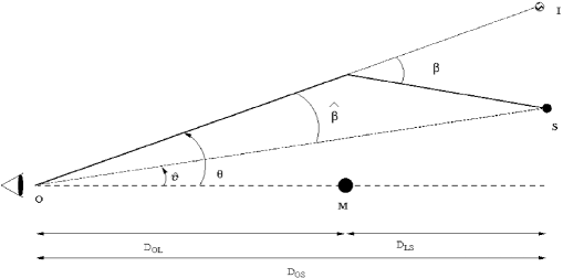
Figure 2: Diagram of the lensing geometry. $\vartheta$ is the angular position of the source; $\theta$ is the angular position of an image; and $D_{OL}$,$D_{OS}$ and $D_{LS}$ are the observe-lens, observer-source and lens-source distances, respectively

.

From the figure, elementary trigonometry establishes the lens equation:

$$\vartheta=\theta-\hat{\beta},$$ (31)

where $\hat{\beta}:=\beta D_{LS}/D_{OS}$.

Since $r_{m}=\theta D_{OL}$ and using equation (31), it then follows that the lens equation takes the form

$$\Theta^{2}-\Theta\left[\varPhi+C_{1}\right]-C_{2}\Theta^{\alpha/2}=0.$$ (32)

where

$$C_{1}:=\frac{\pi}{\theta_{E}}\,\frac{D_{SL}}{D_{OS}}\left[\frac{2\sqrt{1-\alpha}}{2-\alpha}-1\right],\qquad C_{2}:=\theta_{E}^{-\alpha/2}\left(\frac{1}{2}\frac{D_{OS}}{D_{LS}}\right)^{-\alpha/2}\,\sqrt{1-\alpha},$$

and

$$\theta_{E}:=\sqrt{\frac{4GM\,D_{LS}}{D_{OS}\,D_{OL}}},\qquad\Theta:=\frac{\theta}{\theta_{E}},\qquad\varPhi:=\frac{\vartheta}{\theta_{E}}.$$ (33)

The quantities $\Theta$ and $\varPhi$ can be thought of as “scaled angles” with respect to $\theta_{E}$.

In order to solve the lens equation note that, to first order of approximation, the solution can be written as

$$\Theta=\Theta_{0}+\Theta_{1},$$ (34)

where $\Theta_{0}$ represents the standard image position and $\Theta_{1}$ is the correction term to first order. Substitution of equation (34) on (32) gives:

$$\Theta_{1}=\frac{C_{1}\Theta_{0}+C_{2}\Theta_{0}^{\alpha/2}-1}{2\Theta_{0}-\varPhi-C_{1}-\left(\alpha/2\right)C_{2}\,\Theta_{0}^{\alpha/2-1}}.$$ (35)

.

We can now obtain the magnification $\mu:=\theta\mathrm{d}\theta/\vartheta\mathrm{d}\vartheta$ of a lensed image at angular position $\theta$. Using equations (34) and (35) it follows that this magnification is given by

$$\mu=\frac{\Theta_{0}}{\Phi}\frac{\mathrm{d}\Theta_{0}}{\mathrm{d}\Phi}+\frac{\Theta_{1}}{\Phi}\frac{\mathrm{d}\Theta_{0}}{\mathrm{d}\Phi}.$$ (36)

With the known positions and magnifications of the images it is now straightforward to obtain the time delay $\bigtriangleup\tau$ of a light signal. This time is defined as the difference between the light travel time $\tau$ for an actual light ray and the travelled time $\tau_{\text{eu}}$ for an unlensed one, i.e.

$$\delta\tau=\tau-\tau_{\text{eu}}.$$ (37)

To compute the time delay, we use the weak field approximation for the metric, that is $g_{00}\approx 1+2\phi$. For null geodesics it then follows that $\mathrm{d}t=\left(1-\phi\right)\mathrm{d}l$, where $l$ is the Euclidean length. Integrating along to the light ray trajectory and introducing the angular variables $\theta$ and $\vartheta$ we find

$$\delta\tau=\frac{D_{OS}D_{OL}}{D_{LS}}\left[\frac{1}{2}\left(\theta-\vartheta\right)^{2}-\frac{1}{2}\theta_{E}^{2}\ln(\theta/\theta_{E})+\alpha\theta^{2}\ln(\theta/\theta_{E})\right].$$ (38)

According to this, if $\alpha=0$, we obtain the general relativistic time delay. The extra term $\alpha\,\theta^{2}\,\ln(\theta/\theta_{E})$ results in a contribution for it when $\theta$ is greater than $\theta_{E}$. For the case of $\theta=\theta_{E}$, this contribution is null. However, the Einstein angle is not a solution of the lens equation (32) even if $\vartheta=0$, so this case is never achieved. In other words, equation (38) means that the modified time delay is greater than what is obtained in standard general relativity.

6 Conclusion

We have shown that all metric theories of gravity of the form $f(R)=R^{n}$ produce gravitational waves propagating at the velocity of light in vacuum. In particular, the theory developed by Sobouti (2007) satisfies this condition. We have also proved that Sobouti’s theory produces an additional amount of lensing as compared to standard general relativity calculations.

Of course, more investigation on the physical and astrophysical side of the theory developed by Sobouti needs to be done. By no means can his theory be taken as a fundamental one, but rather as a suitable candidate approximation at a certain scale. Particularly, more values of his $\alpha$ parameter need to be calculated for different astronomical environments. Also, more development in the theory of gravitational lensing needs to be done, in order to compare directly with current astronomical data, particularly the anomalous lensing observed in cosmology.

As a final remark, we briefly mention that Sobouti’s theory is not affected by the no–go theorem proposed by Soussa & Woodard (2003) and expanded by Soussa (2003). This is easy to see if we note that some of the components of the perturbations made to the field equations (2) do not necessarily scale with $h^{2}:=h_{\mu\nu}\,h^{\mu\nu}$. In fact, in the weak field approximation, the time–component of equation (2) takes the form

$$\frac{4}{3}\nabla^{2}\phi-2\alpha\left[-\frac{5}{6}+\frac{\ln\left(3\alpha\right)}{3}\right]\nabla^{2}\phi+\frac{2\alpha}{3}\nabla^{2}\phi\,\ln\left(-2\nabla^{2}\phi\right)=\frac{16\pi G\rho}{3}.$$ (39)

From this equation and the value of $\alpha$ given by equation (30) it is clear that the gravitational potential $\phi$ may scale as $\sqrt{GM}$ without ever reaching terms of the order of $h^{2}$. This is the reason of why Sobouti’s theory does not satisfy the conditions of the no–go theorem and so, may account for an extra amount of lensing as explained before.

While this article was being refereed, and since its appearance in the arXiv, a short comment was made by Saffari (2007). This author states that some of the calculations made by Sobouti (2007) are wrong and this is reflected in the circular velocity with a change of sign in one of its terms. In his conclusions he states that, although the main results obtained by Sobouti are not strongly changed, they may affect higher order corrections of the theory and in the limit applicable to very compact objects. Although our article does not reproduce Sobouti’s equations mentioned by Saffari, we were very well aware of the small error made by Sobouti. In fact, the corrections to Sobouti’s calculations have been published in the Thesis made by Rosas–Guevara (2006) (see equations (4.17), (4.20)-(4.24) of Rosas–Guevara Thesis and compare them with equations (2)-(8) in Saffari’s article). So, all the results discussed in the present article are not affected in any manner by the small error made by Sobouti, because the corrections were already included.

Although Sobouti’s theory seems very attractive it has a small caveat which was discussed by him: “Actions are ordinarily form invariant under the changes in sources. Mass dependence of $\alpha$ (cf. equation (30)) destroys this feature and the claim for the action–based theory should be qualified with such reservation in mind”. While this fact is not enough to rule out the theory proposed by Sobouti, one must not forget it.

In summary, it all seems that Sobouti’s theory may play the role of a good candidate for a modified theory of gravity that can be used in the understanding of different astrophysical phenomena, usually described by dark matter. The simplest way to do this in the future is by direct comparisons with observed gravitational lenses (particularly Einstein’s rings) in clusters of galaxies. We are working in this direction and the results obtained will be published elsewhere.

7 Acknowledgements

We thank X. Hernandez for the many discussions, suggestions and comments made to the first draft of this article. We are also grateful to J. Bekenstein for his comments regarding the bending angle and its potential significance at cosmological scales. We very much appreciate the deep comments made by Y. Sobouti, particularly in writing down explicitly the result to $\text{O}(\alpha)$ of equation (28), i.e. relation (29). We also thank L.A. Torres for his comments made to the first draft of the article. We acknowledge the final reading of the article, including its calculations, to T. Bernal. We thank an anonymous referee for his comments which improved the final version of the paper. The authors gratefully acknowledge financial support from DGAPA–UNAM (IN119203) and (IN11307-3). S. Mendoza also acknowledges financial support from CONACyT (41443).

References

- Bekenstein (2004) Bekenstein, J. D. 2004, Phys. Rev. D, 70, 083509
- Bekenstein (2006) Bekenstein, J. D. 2006, Contemporary Physics, 47, 387
- Bertone et al. (2005) Bertone, G., Hooper, D., & Silk, J. 2005, Phys. Rept., 405, 279
- Capozziello (2002) Capozziello, S. 2002, Int. J. Mod. Phys. D., 11, 483
- Capozziello et al. (2003) Capozziello, S., Cardone, V., Carloni, S., & Troisi, A. 2003, Int. J. Mod. Phys. D., 12, 1969
- Capozziello et al. (2006) Capozziello, S., Cardone, V. F., & Troisi, A. 2006, Journal of Cosmology and Astro-Particle Physics, 8, 1
- Capozziello et al. (2006) Capozziello, S., Cardone, V. F., & Troisi, A. 2006, astro-ph/0603522
- Capozziello & Troisi (2005) Capozziello, S. & Troisi, A. 2005, Phys. Rev. D, 72, 044022
- Carroll et al. (2004) Carroll, S., Duvvuri, V., Trodden, M., & Turner, M. 2004, Phys. Rev. D, 70, 2839
- Cognola et al. (2005) Cognola, G., Elizalde, E., Nojiri, S., Odintsov, S. D., & Zerbini, S. 2005, Journal of Cosmology and Astro-Particle Physics, 2, 10
- Cooley (2006) Cooley, J. 2006
- Landau & Lifshitz (1994) Landau, L. & Lifshitz, E. 1994, Course of Theoretical Physics, Vol. 2, The Classical Theory of Fields, 4th edn. (Pergamon)
- Milgrom (1983) Milgrom, M. 1983, ApJ, 270, 365
- Muñoz (2004) Muñoz, C. 2004, Int. J. Mod. Phys., 3093
- Nojiri & Odintsov (2003) Nojiri, S. & Odintsov, S. D. 2003, Phys. Rev. D, 68, 123512
- Nojiri & Odintsov (2004) Nojiri, S. & Odintsov, S. D. 2004, General Relativity and Gravitation, 36, 1765
- Nojiri & Odintsov (2006) Nojiri, S. & Odintsov, S. D. 2006
- Rosas–Guevara (2006) Rosas–Guevara, Y. M. 2006, B.Sc. dissertation, Universidad Nacional Autónoma de México, dissertation available at http://cosmos.astroscu.unam.mx/sergio/students/2005/rosas and at http://bc.unam.mx
- Saffari (2007) Saffari, R. 2007, arXiv:0704.3345v1 [astro-ph]
- Sobouti (2007) Sobouti, Y. 2007, A&A, 464, 921
- Soussa (2003) Soussa, M. E. 2003, astro-ph/0310531
- Soussa & Woodard (2003) Soussa, M. E. & Woodard, R. P. 2003, Classical and Quantum Gravity, 20, 2737