Resonant Compton Upscattering in Anomalous X-ray Pulsars

Abstract

A significant new development in the study of Anomalous X-ray Pulsars (AXPs) has been the recent discovery by INTEGRAL and RXTE of flat, hard X-ray components in three AXPs. These non-thermal spectral components differ dramatically from the steeper quasi-power-law tails seen in the classic X-ray band in these sources. A prime candidate mechanism for generating this new component is resonant, magnetic Compton upscattering. This process is very efficient in the strong magnetic fields present in AXPs. Here an introductory exploration of an inner magnetospheric model for upscattering of surface thermal X-rays in AXPs is offered, preparing the way for an investigation of whether such resonant upscattering can explain the 20-150 keV spectra seen by INTEGRAL. Characteristically flat emission spectra produced by non-thermal electrons injected in the emission region are computed using collision integrals. A relativistic QED scattering cross section is employed so that Klein-Nishina reductions are influential in determining the photon spectra and fluxes. Spectral results depend strongly on the magnetospheric locale of the scattering and the observer’s orientation, which couple directly to the angular distributions of photons sampled.

1 Introduction

Over the last decade, there has been a profound growth in evidence for a new class of isolated neutron stars with ultra-strong magnetic fields, so-called magnetars that include Soft-Gamma Repeaters (SGRs) and Anomalous X-ray Pulsars (AXPs). Such a class was first postulated as a model for SGRs by Duncan & Thompson (1992), and later for AXPs (Thompson & Duncan 1996). The AXPs, are a group of six or seven pulsating X-ray sources with periods around 6-12 seconds. They are bright, possessing luminosities $\,L_{\hbox{\sevenrm X}}\sim 10^{35}\,\rm erg\;s^{-1}\,$, show no sign of any companion, are steadily spinning down and have ages $\,\tau\mathrel{\mathchoice{\lower 2.0pt\vbox{\halign{$\m@th\displaystyle\hfil#\hfil$\cr<\crcr\sim\crcr}}}{\lower 2.0pt\vbox{\halign{$\m@th\textstyle\hfil#\hfil$\cr<\crcr\sim\crcr}}}{\lower 2.0pt\vbox{\halign{$\m@th\scriptstyle\hfil#\hfil$\cr<\crcr\sim\crcr}}}{\lower 2.0pt\vbox{\halign{$\m@th\scriptscriptstyle\hfil#\hfil$\cr<\crcr\sim\crcr}}}}10^{5}\,$ years (e.g. Vasisht & Gotthelf 1997). The steady X-ray emission has been clearly observed in a number of AXPs (e.g. see Tiengo et al. 2002, for XMM observations of 1E 1048.1-5937; Juett et al. 2002 and Patel et al. 2003, for the Chandra spectrum of 4U 0142+61), and also SGRs (see Kulkarni et al. 2003 for Chandra observations of the LMC repeater, SGR 0526-66). A nice summary of spectral fitting of ASCA X-ray data from both varieties of magnetars is given in Perna et al. (2001). This emission displays both thermal contributions, which have $\,kT\sim 0.5-1\,$ keV and so are generally hotter than those in isolated pulsars, and also non-thermal components with steep spectra that can be fit by power-laws $\,dn/dE\propto E^{-s}\,$ of index in the range $\,s=2-3.5\,$.

Flux variability in AXPs is generally small, suggesting that even the non-thermal components experience a moderating influence of the stellar surface, rather than some more dynamic dissipation in the larger magnetosphere. Yet the recent observation (Gavriil & Kaspi 2004) of long-lived pulsed flux flares on the timescale of several months in AXP 1E 1048.1-5937 resembles earlier reports (Baykal & Swank 1996; Oosterbroek et al. 1998) of modest flux instability. There are also correlated long term variations in X-ray flux and non-thermal spectral index in the source 1RXS J170849.0-400910, as identified by Rea et al. (2005). Moreover, Kaspi et al. (2003) and Gavriil, Kaspi & Woods (2002, 2004) reported bursting activity in the AXPs 1E 2259+586 and 1E 1048.1-5937, suggesting that anomalous X-ray pulsars are indeed very similar to SGRs, a “unification paradigm” that is currently gathering support, but remains to be established.

The recent detection by INTEGRAL and RXTE of hard, non-thermal pulsed tails in three AXPs has provided an exciting new twist to the AXP phenomenon. In all of these, the differential spectra above 20 keV are extremely flat: 1E 1841-045 (Kuiper, Hermsen & Mendez 2004) has a power-law energy index of $\,s=0.94\,$ between around 20 keV and 150 keV, 4U 0142+61 displays an index of $\,s=0.2\,$ in the 20 keV – 50 keV band, with a steepening at higher energies implied by the total DC+pulsed spectrum (Kuiper et al. 2006), and RXS J1708-4009 has $\,s=0.88\,$ between 20 keV and 150 keV (Kuiper et al. 2006); these spectra are all much flatter than the non-thermal spectra in the $\,<10\,$ keV band. Also, no clear tail has been seen in 1E 2259+586, yet there is a suggestion of a turn-up in its spectrum in the interval 10–20 keV (Kuiper et al. 2006). The identification of these hard tails was enabled by the IBIS imager on INTEGRAL and secured by a review of archival RXTE PCA and HEXTE data. These tails do not continue much beyond the IBIS energy window, since there are strongly constraining upper bounds from Comptel observations of these sources that necessitate a break and steepening somewhere in the 150–750 keV band (see Figures 4, 7 and 10 of Kuiper et al. 2006). Interestingly, Molkov et al. (2004) and Mereghetti et al. (2004) also reported evidence for hard tails in SGR 1806-20, so that the considerations here are germane also to SGRs in quiescence.

Explaining the generation of these hard tails forms the motivation for this paper, which presents an initial exploration of the production of non-thermal X-rays by inverse Compton heating of soft, atmospheric thermal photons by relativistic electrons. The electrons are presumed to be accelerated either along open or closed field lines, perhaps by electrodynamic potentials, or large scale currents associated with twists in the magnetic field structure (e.g. see Thompson & Beloborodov 2005). In order to power the AXP emission, they must be produced with highly super-Goldreich-Julian densities. In the strong fields of the inner magnetospheres (i.e. within 10 stellar radii) of AXPs, the inverse Compton scattering is predominantly resonant at the cyclotron frequency, with an effective cross section above the classical Thomson value. Hence, proximate to the neutron star surface, in regions bathed intensely by the surface soft X-rays, this process can be extremely efficient for an array of magnetic colatitudes. Here, an investigation of the general character of emission spectra is presented, using collision integral analyses that will set the scene for future explorations using Monte Carlo simulations. This scenario forms an alternative to recent proposals (Thompson & Beloborodov 2005; Heyl & Hernquist 2005) that the new components are of synchrotron or bremsstrahlung origin, and at higher altitudes than considered here. The efficiency of the resonant Compton process suggests it will dominate these other mechanisms if the site of electron acceleration is sufficiently near the stellar surface. This prospect motivates the investigation of resonant inverse Compton models.

2 The Compton Resonasphere

2.1 Energetics

The scattering scenario for AXP hard X-ray tail formation investigated here assumes that the seed energization of electrons arises within a few stellar radii of the magnetar surface. This can in principal occur on either open or closed field lines, so both possibilities will be entertained. The key requirement is the presence of ultra-relativistic electrons moving along B, with an abundance satisfying the energetics of AXPs implied by their intense X-ray luminosities, $\,L_{\hbox{\sevenrm X}}\mathrel{\mathchoice{\lower 2.0pt\vbox{\halign{$\m@th\displaystyle\hfil#\hfil$\cr>\crcr\sim\crcr}}}{\lower 2.0pt\vbox{\halign{$\m@th\textstyle\hfil#\hfil$\cr>\crcr\sim\crcr}}}{\lower 2.0pt\vbox{\halign{$\m@th\scriptstyle\hfil#\hfil$\cr>\crcr\sim\crcr}}}{\lower 2.0pt\vbox{\halign{$\m@th\scriptscriptstyle\hfil#\hfil$\cr>\crcr\sim\crcr}}}}10^{35}\,$erg/sec above 10 keV (Kuiper et al. 2006). The hard X-ray tails have luminosities that are 2–3 orders of magnitude greater than the classical spin-down luminosity $\,{\dot{E}}_{\hbox{\fiverm SD}}\sim 8\pi^{4}B_{p}^{2}R^{6}/(3P^{4}c^{3})\,$ due to magnetic dipole radiation torques. Here $\,B_{p}\,$ is the surface polar field strength. This signature indicates that other dissipation mechanisms, such as structural rearrangements of crustal magnetic fields, power the AXP emission (e.g. Thompson & Duncan 1995; 1996). Let $\,n_{e}\,$ be the number density of such electrons, $\,\langle\gamma_{e}\rangle\,$ be their mean Lorentz factor, and $\,\epsilon_{\hbox{\sevenrm rad}}\,$ be the efficiency of them radiating during their traversal of the magnetosphere (either along open or closed field lines). Then one requires that $\,L_{\hbox{\sevenrm X}}\sim\epsilon_{\hbox{\sevenrm rad}}\langle\gamma_{e}\rangle m_{e}c^{2}(4\pi n_{e}R_{c}^{2}c)\,$ if the emission column has a base that is a spherical cap of radius $\,R_{c}\,$. This yields number densities $\,n_{e}\sim 3\times 10^{17}L_{\hbox{\sevenrm X,35}}/\epsilon_{\hbox{\sevenrm rad}}\langle\gamma_{e}\rangle\,$ cm^-3 for scaled luminosities $\,L_{\hbox{\sevenrm X,35}}\equiv L_{\hbox{\sevenrm X}}/10^{35}\,$erg/sec, if $\,R_{c}\sim 10^{6}\,$cm. Therefore large densities are needed, though not impossible ones, since optically thin conditions for the surface thermal X-rays prevail provided that $\,\langle\gamma_{e}\rangle\gg 1\,$, and $\,\epsilon_{\hbox{\sevenrm rad}}\,$ is not miniscule.

Comparing $\,en_{e}\,$ to the classic Goldreich-Julian (1969) density $\,\rho_{\hbox{\fiverm GJ}}=\nabla.\vec{E}/4\pi=-\vec{\Omega}.\vec{B}/(2\pi c)\,$ for force-free, magnetohydrodynamic rotators, one arrives at the ratio

$$\hbox{${{\displaystyle en_{e}\vphantom{(}}\over{\displaystyle|\rho_{\hbox{\fiverm GJ}}|\vphantom{(}}}$}\;\approx\;\hbox{${{\displaystyle 4,670\vphantom{(}}\over{\displaystyle\epsilon_{\hbox{\sevenrm rad}}\langle\gamma_{e}\rangle\vphantom{(}}}$}\;\hbox{${{\displaystyle L_{X,35}\,P\vphantom{(}}\over{\displaystyle B_{15}R_{6}^{2}\vphantom{(}}}$}\quad,$$ (1)

for AXP pulse periods $\,P\,$ in units of seconds, polar magnetic fields $\,B_{15}\,$ in units of $\,10^{15}\,$Gauss, and cap radii $\,R_{6}\,$ in units of $\,10^{6}\,$cm. Large electron Lorentz factors of $\,\gamma_{e}\gg 10^{2}-10^{3}\,$ and their efficient resonant Compton cooling (i.e. $\,\epsilon_{\hbox{\sevenrm rad}}\sim 0.01-1\,$) are readily attained in isolated pulsars with $\,B\sim 0.1\,$ (e.g. see Sturner 1995; Harding & Muslimov 1998; Dyks & Rudak 2000), and such conditions are expected to persist into the magnetar field regime. For $\,\epsilon_{\hbox{\sevenrm rad}}\langle\gamma_{e}\rangle\mathrel{\mathchoice{\lower 2.0pt\vbox{\halign{$\m@th\displaystyle\hfil#\hfil$\cr>\crcr\sim\crcr}}}{\lower 2.0pt\vbox{\halign{$\m@th\textstyle\hfil#\hfil$\cr>\crcr\sim\crcr}}}{\lower 2.0pt\vbox{\halign{$\m@th\scriptstyle\hfil#\hfil$\cr>\crcr\sim\crcr}}}{\lower 2.0pt\vbox{\halign{$\m@th\scriptscriptstyle\hfil#\hfil$\cr>\crcr\sim\crcr}}}}10^{3}\,$ and $\,R_{6}\sim 1\,$, the requisite density $\,n_{e}\,$ is super-Goldreich-Julian, but not dramatically so. This situation corresponds, however, to acceleration zone cap radii $\,R_{c}\,$ that are considerably larger than standard polar cap radii $\,R\theta_{\hbox{\sevenrm cap}}\,$ for AXPs. Here $\,\theta_{\hbox{\sevenrm cap}}=\arcsin\{(2\pi R/Pc)^{1/2}\}\,$ for a pulsar of radius $\,R\,$ and period $\,P\,$. For $\,P=10\,$sec, this yields $\,R\theta_{\hbox{\sevenrm cap}}\sim 4.6\times 10^{3}\,$cm. Concentrating the relativistic electrons in such a narrow column yields charge densities far exceeding the Goldreich-Julian benchmark implied by Eq. (1). However, since AXPs possess luminosities $\,L_{\hbox{\sevenrm X}}\gg{\dot{E}}_{\hbox{\fiverm SD}}\,$, profound collatitudinal confinement may not prove necessary. Energetically, non-dipolar structure at the surface is easily envisaged, since the dissipation mechanism that powers AXP emission can restructure the fields; there is suggestive evidence for these reconfigurations from variations seen in the pulse profiles, particularly after flaring activity (e.g. see Kaspi et al. 2003). The electron energization zone may then cover a much larger range of colatitudes than is assigned to a standard polar cap, and may extend to closed field lines in equatorial regions. Of course, deviations from dipole structure will modify the contours for the resonasphere considerably from those illustrated just below, though mostly in the inner magnetosphere.

2.2 Resonant Compton Scattering

In strong neutron star fields the cross section for Compton scattering is resonant at the cyclotron energy and a series of higher harmonics (e.g. see Daugherty & Harding 1986), effectively increasing the magnitude of the process over the Thomson cross section  $\sigma_{\hbox{\fiverm T}}$  by as much as the order of $\,1/(\alpha_{\hbox{\sevenrm f}}B)\,$, where $\,\alpha_{\hbox{\sevenrm f}}\,$ is the fine structure constant. Here, as throughout the paper, magnetic fields are written in units of $\,B_{\rm cr}=m_{e}^{2}c^{3}/(e\hbar)=4.413\times 10^{13}\,$Gauss, the quantum critical field strength. Klein-Nishina-like declines operate in supercritical fields, reducing the effective cross section at the resonance (e.g. Gonthier et al. 2000). In the non-relativistic, Thomson regime (e.g. see Herold 1979), only the fundamental resonance is retained. For the specific case of ultra-relativistic electrons colliding with thermal X-rays, in the electron rest frame (ERF), the photons initially move mostly almost along B, and the cyclotron fundamental is again the only resonance that contributes (Gonthier et al. 2000).

The dominance of this resonance in forming upscattering spectra leads to an effective kinematic coupling between the energies $\,\varepsilon_{\gamma}m_{e}c^{2}\,$ and $\,\gamma_{e}m_{e}c^{2}\,$ of colliding photons and electrons, respectively, and the angle of the initial photon $\,\theta_{\gamma}\,$ to the magnetic field lines: the cyclotron fundamental is sampled when

$$\gamma_{e}\varepsilon_{\gamma}(1-\cos\theta_{\gamma})\;\approx\;B\quad,\quad\hbox{for}\;\gamma_{e}\;\gg\;1\quad.$$ (2)

The simplicity of this coupling automatically implies that integration over an angular distribution of incoming photons results in a flat-topped emission spectrum for Compton upscattering of isotropic photons in strong magnetic fields. This characteristic is well-documented in the literature in the magnetic Thomson limit (e.g. see Dermer 1990; Baring 1994; for old gamma-ray burst scenarios, and Daugherty & Harding 1989; Sturner, Dermer & Michel 1995 for pulsar contexts), specifically for collisions between $\,\gamma_{e}\gg 1\,$ electrons and thermal X-rays emanating from a neutron star surface.

It is instructive to compute the zones of influence of the resonant Compton process for magnetic dipole field geometry. For X-ray photons with momentum vector $\,\vec{k}\,$, emanating from a single point at position vector $\,\vec{R}_{e}\,$ on the stellar surface with colatitude $\,\theta_{e}\,$ (i.e., $\,\theta_{e}=0\,$ corresponds to the magnetic pole), the kinematic criterion in Eq. (2) selects out a single photon angle $\,\theta_{\gamma}\,$ for a given local $\,B\,$, both of which are dependent on the altitude and colatitude of the point of interaction. This assumes that the photon propagates with no azimuthal component to its momentum, a specialization that will be remarked upon shortly. In the absence of rotation, the resonance criterion defines a surface that is azimuthally symmetric about the magnetic field axis. The locus of the projection of this surface onto a plane intersecting the magnetic axis can be found through elementary geometry, assuming a flat spacetime. Observe that light bending due to the stellar gravitational potential will modify these loci significantly in inner equatorial regions. At an altitude $\,r\,$ and colatitude $\,\theta\,$, denoted by position vector $\,\vec{r}\,$, the magnetic dipole polar coordinate components are

$$B_{r}\;=\;\hbox{${{\displaystyle B_{p}R^{3}\vphantom{(}}\over{\displaystyle r^{3}\vphantom{(}}}$}\,\cos\theta\quad,\quad B_{\theta}\;=\;\hbox{${{\displaystyle B_{p}R^{3}\vphantom{(}}\over{\displaystyle 2r^{3}\vphantom{(}}}$}\,\sin\theta\quad,$$ (3)

where $\,R\,$ is the neutron star radius and $\,B_{p}\,$ is the surface field strength at the magnetic pole. At this location $\,\vec{r}\,$, the corresponding polar coordinate components $\,k_{r}\,$ and $\,k_{\theta}\,$ of the photon momentum are given by

$${{\displaystyle k_{r}\vphantom{(}}\over{\displaystyle|\vec{k}|\vphantom{(}}} = \hbox{${{\displaystyle\chi-\cos(\theta-\theta_{e})\vphantom{(}}\over{\displaystyle\sqrt{1-2\chi\cos(\theta-\theta_{e})+\chi^{2}}\vphantom{(}}}$}\quad,$$

$${{\displaystyle k_{\theta}\vphantom{(}}\over{\displaystyle|\vec{k}|\vphantom{(}}} = \hbox{${{\displaystyle\sin(\theta-\theta_{e})\vphantom{(}}\over{\displaystyle\sqrt{1-2\chi\cos(\theta-\theta_{e})+\chi^{2}}\vphantom{(}}}$}\quad,$$

where $\,\chi=r/R\,$ is the scaled altitude. The geometry of the magnetic dipole then uniquely determines the angle $\,\theta_{\gamma}=\theta_{\gamma}(r/R,\,\theta;\,\theta_{e})\,$ of the photon to the field via the relation $\,\cos\theta_{\gamma}=\vec{k}.\vec{B}/|\vec{k}|.|\vec{B}|=(k_{r}B_{r}+k_{\theta}B_{\theta})/|\vec{k}|.|\vec{B}|\,$:

$$\cos\theta_{\gamma}\;=\;\hbox{${{\displaystyle 2\cos\theta[\chi-\cos(\theta-\theta_{e})]+\sin\theta\,\sin(\theta-\theta_{e})\vphantom{(}}\over{\displaystyle\sqrt{1+3\cos^{2}\theta}\;\sqrt{1-2\chi\cos(\theta-\theta_{e})+\chi^{2}}\vphantom{(}}}$}\;.$$ (5)

Inserting this into Eq. (2), for the specific case of $\,\theta_{e}=0\,$, yields the equation for the locus defining the surface of resonant scattering for outward-going electrons:

$$\chi^{3}\;=\;\Psi\;\hbox{${{\displaystyle\sqrt{1+3\cos^{2}\theta}\vphantom{(}}\over{\displaystyle 1-\cos\theta_{\gamma}\vphantom{(}}}$}\quad,\quad\Psi\;=\;\hbox{${{\displaystyle B_{p}\vphantom{(}}\over{\displaystyle 2\gamma_{e}\varepsilon_{\gamma}\vphantom{(}}}$}\quad.$$ (6)

Here $\,\Psi\,$ is the key parameter that scales the altitude of the resonance locale, and typically might be in the range $\,1-10^{3}\,$ for magnetars of $\,\gamma_{e}\sim 10^{2}-10^{4}\,$. Eq. (6) can be rearranged into polynomial form, but must be solved numerically. For the special case of soft photons emitted from the surface pole ($\,\theta_{e}=0\,$), the surfaces of resonant scattering for different $\,\Psi\,$ are illustrated in Fig. 1 as the heavy blue contours. The shadows of the emission point are also indicated to demarcate the propagation exclusion zone for the chosen emission colatitude.

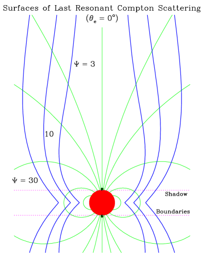
Figure 1: Contours in a section of a pulsar magnetosphere that depict cross sections of the surfaces of last resonant scattering, i.e. the maximal extent of the Compton resonasphere. The heavyweight contours (in dark blue) are computed for different values of the resonance parameter $\,\Psi\,$ defined in Eq. (6), and at extremely high altitudes asymptotically approach the magnetic axis (vertical line). The filled red circle denotes the neutron star, whose radius $\,R\,$ establishes the spatial scale for the figure. The case illustrated is for photons emanating from the polar axis (i.e. $\,\theta_{e}=0^{\circ}\,$), denoted by black dots, for which the neutron star shadow regions are demarcated by the dotted boundaries, and only the surfaces (azimuthally-symmetric about the magnetic axis) are accessible to resonant Compton interactions. In computing the contours, the upscattering electrons were assumed ultra-relativistic, and the depicted spatial scales are linear.

The altitude of resonance is clearly much lower in the equatorial regions, since the photons tend to travel more across field lines in the observer’s frame, and so access the resonance in regions of higher field strength. In contrast, at small colatitudes above the magnetic pole, $\,\theta_{\gamma}\,$ is necessarily small, pushing the resonant surface to very high altitudes where the field is much lower. In this case, the loci asymptotically approach the polar axis at infinity, satisfying $\,\chi^{3}\sin^{2}\theta\approx 16\Psi\,$ for the depicted case of $\,\theta_{e}=0\,$. For $\,\theta_{e}\neq 0\,$ cases (not depicted), the contours are morphologically similar, though they incur significant deviations from those in Fig. 1, both in equatorial and polar regions; for example, when $\,\theta\to 0\,$, the loci do not extend to infinity for $\,\theta_{e}>0\,$. Clearly, by sampling different emission colatitudes $\,\theta_{e}\,$ these surfaces are smeared out into annular volumes. Furthermore, since most photons not emitted at the poles possess azimuthal components to their momenta, propagation out of the plane of the diagram must also be considered, modifying Eqs. (5) and (6). In the interests of compactness, such algebra is not offered here. It suffices to observe that introducing an azimuthal component to the photon momentum generally tends to increase propagation across the field in the observer’s frame, i.e. increasing $\,\theta_{\gamma}\,$, so that the resonance criterion in Eq. (2) is realized at lower altitudes and higher field locales. Hence, taking into account azumithal contributions to photon propagation in the magnetosphere, loci like those depicted in Fig. 1 actually represent the outermost extent of resonant interaction, and so are surfaces of last resonant scattering, i.e. the outer boundaries to the Compton resonasphere. It is evident that, for the majority of closed field lines for long period AXPs, this resonasphere is confined to within a few stellar radii of the surface. Clearly, introducing more complicated, non-dipolar field topologies will also tend to lower the altitudes of the resonasphere.

3 Compton Upscattering Spectra in AXPs

To gain an initial idea of what emission spectra might be produced in the resonasphere of AXPs, collision integral calculations of upscattering spectra are performed. Here results are presented for monoenergetic electrons of Lorentz factor $\,\gamma_{e}\,$, from which spectral forms for various electron distributions can easily be inferred. This approach forgoes considerations of electron cooling, which naturally generates quasi-power-law distributions, at least in the magnetic Thomson limit (e.g. see Dermer 1990; Baring 1994); such issues will be addressed for supercritical fields in future presentations. To simplify the formalism for the spectra, monoenergetic incident photons of dimensionless energy $\,\varepsilon_{\gamma}=\varepsilon_{s}\,$ will be assumed, with the implicit understanding that $\,\varepsilon_{s}\sim 3kT/m_{e}c^{2}\,$, so that values of $\,\varepsilon_{s}\sim 0.003\,$ are commensurate with thermal photon temperatures $\,kT\sim 0.5-1\,$keV observed in AXPs (see Perna et al. 2001). Distributing $\,\varepsilon_{s}\,$ via a Planck spectrum provides only small changes to the spectra illustrated here, serving only to smear out modest spectral structure at the uppermost emergent photon energies.

Central to the characteristics of the spectral shape for resonant upscattering problems are the kinematics associated with both the Lorentz transformation from the observer’s or laboratory frame (OF) to the electron rest frame (ERF), and the scattering kinematics in the ERF. Since choices of photon angles in the two reference frames are not unique, a statement of the conventions adopted here is now made to remove any ambiguities. Let the electron velocity vector in the OF be $\,\vec{\beta}_{e}\,$. This will be parallel to B due to rampant cyclo-synchrotron cooling perpendicular to the field. The dimensionless pre- and post-scattering photon energies (i.e. scaled by $\,m_{e}c^{2}\,$) in the OF are $\,\varepsilon_{i}\,$ and $\,\varepsilon_{f}\,$, respectively, and the corresponding angles of these photons with respect to $\,-\vec{\beta}_{e}\,$ (i.e. field direction) are $\,\Theta_{i}\,$ and $\,\Theta_{f}\,$, respectively. Observe that $\,\Theta_{i}\to\theta_{\gamma}\,$ establishes a connection to the notation used in Section 2. With this definition,

$$\cos\Theta_{i,f}\;=\;-\hbox{${{\displaystyle\vec{\beta}_{e}.\vec{k}_{i,f}\vphantom{(}}\over{\displaystyle|\vec{\beta}_{e}|.|\vec{k}_{i,f}|\vphantom{(}}}$}\quad,$$ (7)

and the zero angles are chosen anti-parallel to the electron velocity. Here, $\,\vec{k}_{i}\,$ and $\,\vec{k}_{f}\,$ are the initial and final photon three-momenta in the OF. Boosting by $\,\vec{\beta}_{e}\,$ to the ERF then yields pre- and post-scattering photon energies in the ERF of $\,\omega_{i}\,$ and $\,\omega_{f}\,$, respectively, with corresponding angles with respect to $\,-\vec{\beta}_{e}\,$ of $\,\theta_{i}\,$ and $\,\theta_{f}\,$. The relations governing this Lorentz transformation are

$$\omega_{i,f}\;=\;\gamma_{e}\varepsilon_{i,f}(1+\beta_{e}\cos\Theta_{i,f})\quad,$$

(8)

$$\cos\theta_{i,f}\;=\;\hbox{${{\displaystyle\cos\Theta_{i,f}+\beta_{e}\vphantom{(}}\over{\displaystyle 1+\beta_{e}\cos\Theta_{i,f}\vphantom{(}}}$}\quad.$$

The inverse transformation relations are obtained from these by the interchange $\,\theta_{i,f}\leftrightarrow\Theta_{i,f}\,$ and the substitutions $\,\omega_{i,f}\to\varepsilon_{i,f}\,$ and $\,\beta_{e}\to-\beta_{e}\,$. The form of Eq. (8) guarantees that for most $\,\Theta_{i}\,$, the initial scattering angle $\,\theta_{i}\,$ in the ERF is close to zero when $\,\gamma_{e}\gg 1\,$, exceptions being cases when $\,\cos\Theta_{i}\approx-\beta_{e}\,$. These exceptional cases form a small minority of the upscattering phase space, and indeed a small contribution to the emergent spectra, and so are safely neglected in the ensuing computations. This $\,\theta_{i}\approx 0\,$ approximation yields dramatic simplification of the differential cross section for resonant Compton scattering, and motivates the particular laboratory frame angle convention adopted in Eq. (7).

The scattering kinematics in the ERF differ from that described by the familiar Compton formula in the absence of magnetic fields (e.g. see Herold 1979; Daugherty & Harding 1986). In the special case $\,\theta_{i}\approx 0\,$ that is generally operable for the scattering scenario here, the kinematic formula for the final photon energy $\,\omega_{f}\,$ in the ERF can be approximated by

$$\omega_{f}\;=\;\omega^{\prime}(\omega_{i},\,\theta_{f})\;\equiv\;\hbox{${{\displaystyle 2\omega_{i}\,r\vphantom{(}}\over{\displaystyle 1+\sqrt{1-2\omega_{i}r^{2}\sin^{2}\theta_{f}}\vphantom{(}}}$}\quad,$$ (9)

where

$$r\;=\;\hbox{${{\displaystyle 1\vphantom{(}}\over{\displaystyle 1+\omega(1-\cos\theta_{f})\vphantom{(}}}$}$$ (10)

is the ratio $\,\omega_{f}/\omega_{i}\,$ that would correspond to the non-magnetic Compton formula, which in fact does result if $\,\omega_{i}r^{2}\sin^{2}\theta_{f}\ll 1\,$. Eq. (9) can be found in Eq.  (15) of Gonthier et al. (2000), and is realized for the particular case where electrons remain in the ground state (zeroth Landau level) after scattering. Such a situation occurs for the resonant problem addressed in this paper, a feature that is discussed briefly below.

Let $\,n_{\gamma}\,$ be the number density of photons resulting from the resonant scattering process. For inverse Compton scattering, an expression for the spectrum of photon production $\,dn_{\gamma}/(dt\,d\varepsilon_{f}\,d\mu_{f})\,$, differential in the photon’s post-scattering laboratory frame quantities $\,\varepsilon_{f}\,$ and $\,\mu_{f}=\cos\Theta_{f}\,$, was presented in Eqs. (A7)–(A9) of Ho and Epstein (1989), valid for general scattering scenarios, including Klein-Nishina regimes. This was used by Dermer (1990) and Baring (1994) in the magnetic Thomson domain, i.e. when $\,B\ll 1\,$ and the photon energy in the electron rest frame (ERF) is far inferior to $\,m_{e}c^{2}\,$. Such specialization is readily extended to the magnetar regime by incorporating into the Ho and Epstein formalism the magnetic kinematics and the QED cross section for fully relativistic cases. The result can be integrated over $\,\mu_{f}\,$ and then written as

$${{\displaystyle dn_{\gamma}\vphantom{(}}\over{\displaystyle dt\,d\varepsilon_{f}\vphantom{(}}} = \hbox{${{\displaystyle n_{e}n_{s}\,c\vphantom{(}}\over{\displaystyle\mu_{+}-\mu_{-}\vphantom{(}}}$}\int_{\mu_{l}}^{\mu_{u}}d\mu_{f}\int_{\mu_{-}}^{\mu_{+}}d\mu_{i}$$

$$\delta\big{[}\omega_{f}-\omega^{\prime}(\omega_{i},\,\theta_{f})\,\bigl{]}\,\hbox{${{\displaystyle 1+\beta_{e}\mu_{i}\vphantom{(}}\over{\displaystyle\gamma_{e}(1+\beta_{e}\mu_{f})\vphantom{(}}}$}\,\hbox{${{\displaystyle d\sigma\vphantom{(}}\over{\displaystyle d(\cos\theta_{f})\vphantom{(}}}$}\quad,$$

noting that the angle convention specified in Eq. (7) requires the substitution $\,\beta_{e}\to-\beta_{e}\,$ in Eqs. (A7–A9) of Ho and Epstein (1989). Here, the notation $\,\mu_{i}=\cos\Theta_{i}\,$ and $\,\mu_{f}=\cos\Theta_{f}\,$ is used for compactness, $\,n_{e}\,$ is the number density of relativistic electrons, and $\,n_{s}\,$ is that for the soft photons. These incident monoenergetic photons are assumed to possess a uniform distribution of angle cosines $\,\mu_{i}\,$ in some range $\,\mu_{-}\leq\mu_{i}\leq\mu_{+}\,$, which is generally broad enough to encompass the resonance, i.e. the value $\,\mu_{i}=[B/(\gamma_{e}\varepsilon_{s})-1]/\beta_{e}\,$. The bounds on the $\,\mu_{f}\,$ integration, defining the observable range of angle cosines with respect to the field direction, will be specialized to $\,\mu_{l}=-1\,$ and $\,\mu_{u}=1\,$ in the illustration here, though dependence of the emergent spectra $\,\Theta_{f}\,$ values will be discussed below. The function $\,\omega^{\prime}(\omega_{i},\,\theta_{f})\,$, which appears in the delta function in Eq. (LABEL:eq:scatt_spec) that encapsulates the scattering kinematics, is that defined in Eq. (9).

Fully relativistic, quantum cross section formalism for the Compton interaction in magnetic fields can be found in Herold (1979), Daugherty & Harding (1986), and Bussard, Alexander & Mészáros (1986). These extend earlier non-relativistic quantum mechanical formulations such as in Canuto, Lodenquai & Ruderman (1971), and Blandford & Scharlemann (1976). The differential cross section, $\,d\sigma/d\cos\theta_{f}\,$, appearing in Eq. (LABEL:eq:scatt_spec) is taken from Eq. (23) of Gonthier et al. (2000), and incorporates the relativistic QED physics. Yet, it is specialized to the case of scatterings that leave the electron in the ground state, the zeroth Landau level that it originates from. This expedient choice is entirely appropriate, since it yields the dominant contribution to the cross section at and below the cyclotron resonance (e.g. Daugherty & Harding 1986; Gonthier et al. 2000). For considerations below, where information on the final polarization state of the photon is retained, Eq. (22) of Gonthier et al. (2000) is used; this simplifies to the forms

$${{\displaystyle d\sigma_{\parallel,\perp}\vphantom{(}}\over{\displaystyle d\cos\theta_{f}\vphantom{(}}} = {{\displaystyle 3\sigma_{\rm T}\vphantom{(}}\over{\displaystyle 32\vphantom{(}}} {{\displaystyle(\omega_{f})^{3}\;T_{\parallel,\perp}\,\exp\bigl{\{}-\omega_{f}^{2}\sin^{2}\theta_{f}/[2B]\bigr{\}}\vphantom{(}}\over{\displaystyle\omega_{i}\,[1+\omega_{i}(1-\cos\theta_{f})-\omega_{f}\sin^{2}\theta_{f}]\vphantom{(}}}$$

$$\times \biggl{\{}\hbox{${{\displaystyle 1\vphantom{(}}\over{\displaystyle(\omega_{i}-B)^{2}+(\Gamma_{\hbox{\sevenrm cyc}}/2)^{2}\vphantom{(}}}$}+\hbox{${{\displaystyle 1\vphantom{(}}\over{\displaystyle(\omega_{i}+B-\zeta)^{2}\vphantom{(}}}$}\biggr{\}}$$

for the differential cross sections, where the cyclotron decay width $\,\Gamma_{\hbox{\sevenrm cyc}}\,$ (discussed below) has been introduced to render the resonance finite in the form of a Lorentz profile. The exponential factor in Eq. (LABEL:eq:sigma_pol) is a relic of the Laguerre functions that signal the discretization of momentum/energy states perpendicular to the field. Furthermore, the factor in square brackets in the denominator is always positive, being proportional to $\,1-\omega_{f}r\sin^{2}\theta_{f}\,$, which can be shown to be precisely the square root appearing in Eq. (9). Also, $\,\zeta=\omega_{i}\omega_{f}(1-\cos\theta_{f})\,$, and

$$T_{\parallel} = 2\cos^{2}\theta_{f}+\omega_{i}(1-\cos\theta_{f})^{2}-\omega_{f}\sin^{2}\theta_{f}$$

$$T_{\perp} = 2+\omega_{i}(1-\cos\theta_{f})^{2}-\omega_{f}\sin^{2}\theta_{f}\quad.$$

Here, the standard convention for the labelling of the photon linear polarizations is adopted: $\,\parallel\,$ refers to the state with the photon’s electric field vector parallel to the plane containing the magnetic field and the photon’s momentum vector, while $\,\perp\,$ denotes the photon’s electric field vector being normal to this plane.

For magnetic Compton scattering, in the particular case of photons propagating along B prior to scattering (i.e. $\,\theta_{i}=0\,$), the differential cross sections are independent of the initial polarization of the photon (Gonthier et al. 2000); this property is a consequence of circular polarizations forming the natural basis states for $\,\theta_{i}=0\,$. Therefore, transitions $\,\perp\to\parallel\,$ and $\,\parallel\to\parallel\,$ yield identical forms for the cross sections, and separately so do the transitions $\,\perp\to\perp\,$ and $\,\parallel\to\perp\,$. Accordingly, the cross sections in Eq. (LABEL:eq:sigma_pol) are labelled only by the post-scattering linear polarization state of the photon; they are summed when polarization-independent results are desired, i.e. $\,d\sigma/d\cos\theta_{f}=(d\sigma_{\parallel}/d\cos\theta_{f}+d\sigma_{\perp}/d\cos\theta_{f})\,$. Therefore, clearly the upscattered photon spectra presented here are insensitive to the initial polarization level (zero or otherwise) of the soft photons.

The integrals in Eq. (LABEL:eq:scatt_spec) can be manipulated using the Jacobian identity $\,d\mu_{i}\,d\mu_{f}=d\omega_{i}\,d\omega_{f}/(\gamma_{e}^{2}\beta_{e}^{2}\varepsilon_{i}\varepsilon_{f})\,$ to change variables to $\,\omega_{i}\,$ and $\,\omega_{f}\,$. Observe that the values of $\,\mu_{\pm}\,$ do not impact these integrations provided that the resonance condition in Eq. (2) is sampled. The $\,\omega_{f}\,$ integration is then trivial. The $\,\omega_{i}\,$ integration is more involved, but can be developed by suitable approximation, as follows. The relativistic Compton cross section is strongly peaked at the cyclotron fundamental (see Fig. 2 of Gonthier et al. 2000) due to the appearance of the resonant denominator $\,1/[(\omega_{i}-B)^{2}+(\Gamma_{\hbox{\sevenrm cyc}}/2)^{2}]\,$, where $\,\Gamma_{\hbox{\sevenrm cyc}}\ll B\,$ is the dimensionless cyclotron decay rate from the first Landau level. Therefore, this Lorentz profile can be approximated by a delta function in $\,\omega_{i}\,$ space of identical normalization in an integration over $\,\omega_{i}\,$:

$$\hbox{${{\displaystyle 1\vphantom{(}}\over{\displaystyle(\omega_{i}-B)^{2}+(\Gamma_{\hbox{\sevenrm cyc}}/2)^{2}\vphantom{(}}}$}\;\to\;\hbox{${{\displaystyle 2\pi\vphantom{(}}\over{\displaystyle\Gamma_{\hbox{\sevenrm cyc}}\vphantom{(}}}$}\,\delta(\omega_{i}-B)\quad.$$ (14)

This mapping, which was adopted in the magnetic Thomson limit by Dermer (1990), renders the $\,\omega_{i}\,$ trivial, with the non-resonant term in the cross section in Eq. (LABEL:eq:sigma_pol) being neglected, and the evaluation of the integrals in Eq. (LABEL:eq:scatt_spec) complete. The spectra scale as the inverse of the decay rate $\,\Gamma_{\hbox{\sevenrm cyc}}\,$, whose form can be found, for example, in Eqs. (13) or (23) of Baring, Gonthier & Harding (2005; see also Latal 1986; Harding & Lai 2006). For $\,B\ll 1\,$, $\,\Gamma_{\hbox{\sevenrm cyc}}\approx 4\alpha_{\hbox{\sevenrm f}}B^{2}/3\,$, which traces classical cyclotron cooling, while for $\,B\gg 1\,$, quantum effects and recoil reductions generate $\,\Gamma_{\hbox{\sevenrm cyc}}\approx(\alpha_{\hbox{\sevenrm f}}/e)\sqrt{B/2}\,$.

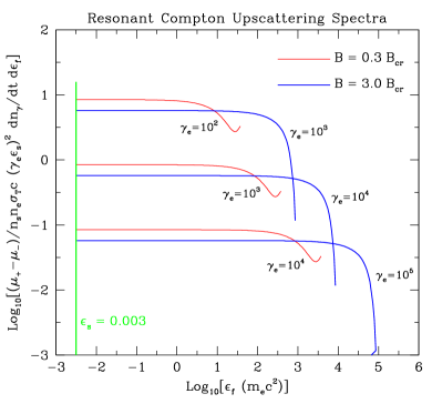
Figure 2: Resonant Compton upscattering spectra (scaled) such as might be sampled in the magnetosphere of an AXP, for different relativistic electron Lorentz factors $\,\gamma_{e}\,$, as labelled. The emergent photon energy $\,\varepsilon_{f}\,$ is scaled in terms of $\,m_{e}c^{2}\,$. The chosen magnetic field strengths of $\,B=3B_{\rm cr}\,$ (heavyweight, blue) and $\,B=0.3B_{\rm cr}\,$ (lighter weight, red) correspond to different altitudes and perhaps colatitudes. Results are depicted for seed photons of energy $\,\varepsilon_{s}=0.003\,$ (marked by the green vertical line), typical of thermal X-rays emanating from AXP surfaces; downscattering resonant emission at $\,\varepsilon_{f}<\varepsilon_{s}\,$ was not exhibited.

Representative spectral forms are depicted in Fig. 2, for the situation where the emergent polarization is not observed. Because of the approximation to the resonance in Eq. (14), non-resonant scattering contributions were omitted when generating the curves; these contributions produce steep wings to the spectra at the uppermost and lowermost energies (not shown), and a slight bolstering of the resonant portion. This resonant restriction suffices for the purposes of this paper, and kinematically limits the range of emergent photon energies $\,\varepsilon_{f}\,$ to

$$\gamma_{e}(1-\beta_{e})\,B\;\leq\;\varepsilon_{f}\;\leq\;\hbox{${{\displaystyle\gamma_{e}(1+\beta_{e})\,B\vphantom{(}}\over{\displaystyle 1+2B\vphantom{(}}}$}\quad.$$ (15)

This range generally extends below the thermal photon seed energy $\,\varepsilon_{s}\,$. Such downscatterings correspond to forward scatterings $\,\cos\theta_{f}\approx 1\,$ in the ERF such that $\,\theta_{f}\mathrel{\mathchoice{\lower 2.0pt\vbox{\halign{$\m@th\displaystyle\hfil#\hfil$\cr<\crcr\sim\crcr}}}{\lower 2.0pt\vbox{\halign{$\m@th\textstyle\hfil#\hfil$\cr<\crcr\sim\crcr}}}{\lower 2.0pt\vbox{\halign{$\m@th\scriptstyle\hfil#\hfil$\cr<\crcr\sim\crcr}}}{\lower 2.0pt\vbox{\halign{$\m@th\scriptscriptstyle\hfil#\hfil$\cr<\crcr\sim\crcr}}}}\theta_{i}\sim 1/\gamma_{e}\,$. Since they constitute a miniscule portion of the angular phase space (and energy budget), only upscattering spectra are exhibited in the Figure.

In the $\,B=0.3\,$ case, a quasi-Thomson regime, the spectra show a characteristic flat distribution that is indicative of the kinematic sampling of the resonance in the integrations (e.g. see Dermer 1990; Baring 1994). For much of this spectral range, forward scattering in the observer’s frame is operating: $\,\mu_{f}=\cos\Theta_{f}\approx 1\,$. This establishes almost Thomson kinematics, with the scattered photon energy in the ERF satisfying $\,\omega_{f}\approx\omega_{i}\,$. Substituting these approximations into Eqs. (LABEL:eq:sigma_pol) and (LABEL:eq:TparTperp), and then summing over final polarizations yields a total approximate form for the flat portions of the spectral production rate in Eq. (LABEL:eq:scatt_spec) for cases $\,\gamma_{e}\gg 1\,$:

$$\hbox{${{\displaystyle dn_{\gamma}\vphantom{(}}\over{\displaystyle dt\,d\varepsilon_{f}\vphantom{(}}}$}\;\approx\;\hbox{${{\displaystyle n_{e}n_{s}\,\hbox{$\sigma_{\hbox{\fiverm T}}$}c\vphantom{(}}\over{\displaystyle\mu_{+}-\mu_{-}\vphantom{(}}}$}\;\hbox{${{\displaystyle 3\pi B^{2}\vphantom{(}}\over{\displaystyle 4\Gamma_{\hbox{\sevenrm cyc}}\,\gamma_{e}^{3}\varepsilon_{s}^{2}\vphantom{(}}}$}\quad.$$ (16)

The magnetic field and $\,\gamma_{e}\,$ dependences are evident in Fig. 2 (remembering that the curves are multiplied by $\,\gamma_{e}^{2}\,$ for the purposes of illustration), and since $\,\Gamma_{\hbox{\sevenrm cyc}}\propto B^{2}\,$ when $\,B\ll 1\,$, the normalization of the flat spectrum is independent of the field strength in the magnetic Thomson regime. Only at the highest energies does the spectrum begin to deviate from flat (i.e. horizontal) behavior, and this domain corresponds to significant scattering angles in the ERF, i.e. cosines $\,1-\cos\theta_{f}\,$ not much less than unity. Then the mathematical form of the differential cross section becomes influential in determining the spectral shape. Specifically, for $\,\theta_{f}\sim\pi/2\,$, $\,T_{\parallel}\,$ drops far below $\,T_{\perp}\,$, as is evident in Eq. (LABEL:eq:TparTperp), causing the observed dip in the spectra. At slightly higher energies $\,\varepsilon_{f}\,$, there is a recovery when $\,T_{\parallel}\,$ rises as $\,\theta_{f}\to\pi\,$. Observe that $\,T_{\perp}\,$ is far less sensitive to scattering angles $\,\theta_{f}\,$ in the ERF, except for supercritical fields when recoil becomes significant. The sum of the two contributions yields a slight cusp at the maximum energy $\,\varepsilon_{f}\approx\gamma_{e}(1+\beta_{e})B/(1+2B)\,$ when $\,B\mathrel{\mathchoice{\lower 2.0pt\vbox{\halign{$\m@th\displaystyle\hfil#\hfil$\cr<\crcr\sim\crcr}}}{\lower 2.0pt\vbox{\halign{$\m@th\textstyle\hfil#\hfil$\cr<\crcr\sim\crcr}}}{\lower 2.0pt\vbox{\halign{$\m@th\scriptstyle\hfil#\hfil$\cr<\crcr\sim\crcr}}}{\lower 2.0pt\vbox{\halign{$\m@th\scriptscriptstyle\hfil#\hfil$\cr<\crcr\sim\crcr}}}}0.5\,$, which disappears for higher fields when the recoil reductions of $\,d\sigma/d\cos\theta_{f}\,$ become dominant.

In AXPs, the $\,B=0.3\,$ case best represents higher altitude locales for the resonasphere, such as at smaller colatitudes near the polar axis. For $\,B=3\,$, more typical of equatorial resonance locales, the flat spectrum still appears at energies $\,\varepsilon_{s}\leq\varepsilon_{f}\ll\gamma_{e}(1+\beta_{e})\,B/(1+2B)\,$, when again $\,\cos\theta_{f}\approx 1\,$. Yet the curves in Fig. 2 display more prominent reductions at the uppermost energies $\,\varepsilon_{f}\sim\gamma_{e}(1+\beta_{e})\,B/(1+2B)\,$ due to the sampling of $\,1/2\leq\omega_{f}\ll\omega_{i}\,$ values in the ERF that correspond to strong electron recoil effects. Photons emitted in this regime have $\,1-\cos\theta_{f}\sim 1\,$ in the ERF and are highly beamed along the field in the observer’s frame, as will become apparent shortly. At these maximum energies, the approximations $\,\cos\theta_{f}\approx 1\,$ and $\,\omega_{f}\approx B/(1+2B)\,$ yield an analytic result for the emission rate, precisely Eq. (16) multiplied by the factor $\,1/(1+2B)^{2}\,$ that controls the severity of the reduction at the uppermost resonant energies. Note that Klein-Nishina reductions in the cross section regulate the overall normalizations of the $\,B=3\,$ curves, as does the fact that the cyclotron width $\,\Gamma_{\hbox{\sevenrm cyc}}\,$ no longer scales with field strength as $\,B^{2}\,$.

The dimensionless electron energy loss rate $\,d\gamma_{e}/dt\,$ can be obtained by multiplying the differential spectrum $\,dn_{\gamma}/dtd\varepsilon_{f}\,$ in Eq. (LABEL:eq:scatt_spec) by $\,\varepsilon_{f}/n_{e}\,$ and integrating over $\,\varepsilon_{f}\,$. Because of the flat nature of the spectrum, this receives a dominant contribution from near the maximum upscattered energy $\,\gamma_{e}(1+\beta_{e})\,B/(1+2B)\,$. Then, using Eq. (16), in the magnetic Thomson limit $\,B\ll 1\,$, since energies $\,\varepsilon_{f}\sim 2\gamma_{e}B\,$ contribute most, the result $\,d\gamma_{e}/dt\propto B^{4}/\Gamma_{\hbox{\sevenrm cyc}}\propto B^{2}\,$ is obviously realized for $\,\Gamma_{\hbox{\sevenrm cyc}}\approx 4\alpha_{\hbox{\sevenrm f}}B^{2}/3\,$. The full integration of Eq. (LABEL:eq:scatt_spec) over $\,\varepsilon_{f}\,$ (or equivalently $\,\cos\theta_{f}\,$) is analytically tractable, leading to

$$\hbox{${{\displaystyle d\gamma_{e}\vphantom{(}}\over{\displaystyle dt\vphantom{(}}}$}\;\approx\;\hbox{${{\displaystyle n_{s}\,\hbox{$\sigma_{\hbox{\fiverm T}}$}c\vphantom{(}}\over{\displaystyle\mu_{+}-\mu_{-}\vphantom{(}}}$}\;\hbox{${{\displaystyle 3\pi B^{2}\vphantom{(}}\over{\displaystyle 4\gamma_{e}\varepsilon_{s}^{2}\vphantom{(}}}$}\quad,\quad B\;\ll\;1\quad.$$ (17)

This result is commensurate with the form derived in Eq. (24) of Dermer (1990). In contrast, when $\,B\gg 1\,$, the overall normalization of the spectrum at energies $\,\varepsilon_{f}\ll\gamma_{e}(1+\beta_{e})B/(1+2B)\,$ is still controlled by Eq. (16), but now the cyclotron decay rate dependence $\,\Gamma_{\hbox{\sevenrm cyc}}\propto B^{1/2}\,$ and recoil reductions at the highest $\,\varepsilon_{f}\,$ come into play, so that the cooling rate $\,d\gamma_{e}/dt\,$ possesses a dependence on the field strength that is much weaker than $\,B^{3/2}\,$.

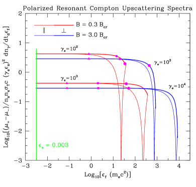
Figure 3: Resonant Compton upscattering spectra appropriate for an AXP magnetosphere, scaled as in Fig. 2, but this time displaying the two polarizations $\,\perp\,$ (heavyweight) and $\,\parallel\,$ (lightweight) for the produced photons; the dominance of the $\,\perp\,$ polarization near the uppermost energies is evident. Again, the emergent photon energy $\,\varepsilon_{f}\,$ is scaled in terms of $\,m_{e}c^{2}\,$, and results are presented for different relativistic electron Lorentz factors $\,\gamma_{e}\,$, as labelled. Specific emergent angles of the emission in the observer’s frame, with respect to the magnetic field direction, are indicated by the filled magenta symbols, with triangles denoting $\,\Theta_{f}=5^{\circ}\,$, squares corresponding to $\,\Theta_{f}=1^{\circ}\,$, and circles representing $\,\Theta_{f}=0.2^{\circ}\,$. The magnetic field strengths of $\,B=3B_{\rm cr}\,$ (blue) and $\,B=0.3B_{\rm cr}\,$ (red) correspond perhaps to lower and higher altitudes, respectively. Again, the green vertical line marks the soft photon energy $\,\varepsilon_{s}=0.003\,$, with downscattering resonant emission at $\,\varepsilon_{f}<\varepsilon_{s}\,$ not being exhibited.

The resonant upscattering spectra are potentially polarized, perhaps strongly. Isolating the specific polarization forms in Eq. (LABEL:eq:TparTperp), the polarization-dependent resonant Compton spectra are readily computed and are illustrated in Fig. 3. It is clear from Eq. (LABEL:eq:TparTperp) that the emissivities for photons of final polarization state $\,\perp\,$ should always be superior to those for the $\,\parallel\,$ state. In a classical description, this is a consequence of the physical ease with which an oscillating electron can resonantly drive emission with electric field vectors perpendicular to B. Yet for much of the range of emergent photon energies above $\,\varepsilon_{s}=0.003\,$, there is no material difference between fluxes for the two final polarizations. This case corresponds to $\,\cos\theta_{f}\approx 1\,$, i.e. photon emission along the field in the ERF, and hence induces zero linear polarization by symmetry, but permits emergent circular polarization. At the highest produced energies, significant differences between $\,\perp\,$ and $\,\parallel\,$ emission appear, with $\,1-\cos\theta_{f}\,$ no longer very small (see Eq. (LABEL:eq:TparTperp) to help identify this characteristic). This domain motivates the development of medium energy gamma-ray polarimeters as a tool for geometry diagnostics.

Another feature of the upscattering process that is highlighted in the Fig. 3 is the intense beaming of radiation along the field in the observer’s frame of reference, and the profound correlation of the angle of emission $\,\Theta_{f}\,$ with the emergent photon energy $\,\varepsilon_{f}\,$. This tight correspondence is mathematically guaranteed by the appearance of the kinematic delta function in Eq. (LABEL:eq:scatt_spec) together with the intrinsically narrow nature of the scattering resonance, which permits the delta function approximation in Eq. (14). The extremely narrow range of $\,\Theta_{f}\,$ for each observed energy $\,\varepsilon_{f}\,$ is broadened when non-resonant scattering is introduced. In the resonant case here, the $\,\gamma_{e}\gg 1\,$ regime dictates that most of the emission is collimated to within $\,5^{\circ}\,$ of the field direction, and rapidly becomes beamed to within $\,0.2^{\circ}\,$ as the final photon energy increases towards its maximum. This kinematic characteristic guarantees that spectral formation in Compton upscattering models is extremely sensitive to the observer’s viewing perspective in relation to the magnetospheric geometry, offering useful probes if pulse-phase spectroscopy is achievable.

It should be noted that the spectra in Figs. 2 and 3 are in principal subject to attenuation by magnetic pair production, $\,\gamma\to e^{+}e^{-}\,$, reprocessing the highest energy photons to lower energies. This process is sensitive to the angle $\,\Theta_{f}\,$ of the scattered photons to the field, which, from the results depicted here, is strongly coupled to their energy $\,\varepsilon_{f}\,$. Gonthier et al. (2000) demonstrated (see their Figure 7) that generally, for an extended range of values for $\,B\,$, pair creation attenuation would only operate for $\,\omega_{i}\mathrel{\mathchoice{\lower 2.0pt\vbox{\halign{$\m@th\displaystyle\hfil#\hfil$\cr>\crcr\sim\crcr}}}{\lower 2.0pt\vbox{\halign{$\m@th\textstyle\hfil#\hfil$\cr>\crcr\sim\crcr}}}{\lower 2.0pt\vbox{\halign{$\m@th\scriptstyle\hfil#\hfil$\cr>\crcr\sim\crcr}}}{\lower 2.0pt\vbox{\halign{$\m@th\scriptscriptstyle\hfil#\hfil$\cr>\crcr\sim\crcr}}}}10\,$–30 in the ERF, since the resonant Compton process couples the values of $\,\omega_{f}\,$ and $\,\theta_{f}\,$. For the resonant scattering considerations here, this criterion translates to $\,\gamma\to e^{+}e^{-}\,$ being rife for local fields $\,B\mathrel{\mathchoice{\lower 2.0pt\vbox{\halign{$\m@th\displaystyle\hfil#\hfil$\cr>\crcr\sim\crcr}}}{\lower 2.0pt\vbox{\halign{$\m@th\textstyle\hfil#\hfil$\cr>\crcr\sim\crcr}}}{\lower 2.0pt\vbox{\halign{$\m@th\scriptstyle\hfil#\hfil$\cr>\crcr\sim\crcr}}}{\lower 2.0pt\vbox{\halign{$\m@th\scriptscriptstyle\hfil#\hfil$\cr>\crcr\sim\crcr}}}}10\,$ and being marginal, or more probably ineffective, at lower field strengths. For $\,B\mathrel{\mathchoice{\lower 2.0pt\vbox{\halign{$\m@th\displaystyle\hfil#\hfil$\cr>\crcr\sim\crcr}}}{\lower 2.0pt\vbox{\halign{$\m@th\textstyle\hfil#\hfil$\cr>\crcr\sim\crcr}}}{\lower 2.0pt\vbox{\halign{$\m@th\scriptstyle\hfil#\hfil$\cr>\crcr\sim\crcr}}}{\lower 2.0pt\vbox{\halign{$\m@th\scriptscriptstyle\hfil#\hfil$\cr>\crcr\sim\crcr}}}}10\,$ scattering circumstances, any pair creation that ensues does so by generating pairs in the ground state (e.g. Usov & Melrose 1995; Baring & Harding 2001), with Lorentz factors less than $\,\gamma_{e}\,$ since $\,\varepsilon_{f}<\gamma_{e}\,$. Accordingly the cascading would consist at first of generations of upscattering and subsequent pair creation, until high enough altitudes are encountered for pair production to access excited Landau levels for the pairs, and then synchrotron/cyclotron radiation can ensue and complicate the cascade.

4 Discussion

It is clear that the spectra exhibited in Fig. 2 are considerably flatter than the hard X-ray tails ($\,\sim\varepsilon_{f}^{-1}\,$) seen in the AXPs, and extend to energies much higher than can be permitted by the Comptel upper bounds to these sources. However, they represent a preliminary indication of how flat the resonant scattering process can render the emergent spectrum, and what an observer detects will depend critically on his/her orientation and the magnetospheric locale of the scattering. The one-to-one kinematic correspondence between $\,\varepsilon_{f}\,$ and $\,\mu_{f}\,$ (illustrated via the filled symbols in Fig. 3), imposed by $\,\omega_{f}=\gamma_{e}\varepsilon_{f}(1-\mu_{f})=\omega^{\prime}(\omega_{i})\,$ with $\,\omega_{i}=B\,$, implies that the highest energy photons are beamed strongly along the local field direction. This may or may not be sampled by an instantaneous observation, which varies with the rotational phase. Realistically, depending on the pulse phase, angles corresponding to $\,\mu_{f}<1\,$ will be predominant, lowering the value of $\,\varepsilon_{f}\,$. Yet how low is presently unclear, and remains to be explored via a model with full magnetospheric geometry, an essential step. One can also expect substantial spectral differences between scattering locales attached to open and closed field lines, and also between dipolar and more complicated field morphologies with smaller radii of curvature.

Distributing the electron $\,\gamma_{e}\,$ such as through resonant cooling will generate a convolution of the spectra depicted in Fig. 2; observe that the $\,\gamma_{e}^{2}\,$ scaling of the y-axis implies that the normalization of the curves is a strongly-declining function of $\,\gamma_{e}\,$. This can clearly steepen the continuum for a particular range of $\,\mu_{f}\,$. For example, since $\,\varepsilon_{f}\propto\gamma_{e}\,$ near the maximum photon energy for a fixed electron Lorentz factor, integration over a truncated $\,\gamma_{e}^{-p}\,$ distribution, where $\,\gamma_{e}\geq\gamma_{e,min}\,$, naturally yields a photon spectrum $\,\varepsilon_{f}^{-(p+2)}\,$ at energies above the critical value $\,\varepsilon_{f}\sim 2\gamma_{e,min}B/(1+2B)\,$ where the resonant flat top turns over. In particular, cooling the electrons as they propagate in the magnetosphere can lead to significant and possibly dominant contributions from Lorentz factors $\,\gamma_{e}\mathrel{\mathchoice{\lower 2.0pt\vbox{\halign{$\m@th\displaystyle\hfil#\hfil$\cr<\crcr\sim\crcr}}}{\lower 2.0pt\vbox{\halign{$\m@th\textstyle\hfil#\hfil$\cr<\crcr\sim\crcr}}}{\lower 2.0pt\vbox{\halign{$\m@th\scriptstyle\hfil#\hfil$\cr<\crcr\sim\crcr}}}{\lower 2.0pt\vbox{\halign{$\m@th\scriptscriptstyle\hfil#\hfil$\cr<\crcr\sim\crcr}}}}10\,$ at higher altitudes and lower $\,B\,$ that can evade the Comptel constraints on the AXPs (see Kuiper et al. 2006). In the Thomson regime, the cooling tends to steepen the continuum (e.g. Baring 1994) in the X-ray band due to a pile-up of electrons at low $\,\gamma_{e}\,$. If electrons propagate to high altitudes in magnetars, a similar steepening should be expected. As the polarized signal appears at the highest energies for each $\,\gamma_{e}\,$, a somewhat broad range of energies will exhibit polarization above around 50–100 keV when integrating over an entire cooled electron distribution. Note also that the cooling may persist down to mildly-relativistic energies, i.e., $\,\gamma_{e}\sim 1\,$, in which case it can seed a multiple scattering Comptonization of thermal X-rays that may generate the steep non-thermal continuum observed in AXPs below 10 keV. Such resonant, magnetic Comptonization has been explored by Lyutikov & Gavriil (2006), and provides very good fits to both Chandra (Lyutikov & Gavriil 2006) and XMM (see Rea et al. 2006) spectral data for the AXP 1E 1048.1-5937.

Finally, the introduction of non-resonant contributions can have a significant impact on the spectral shape. The resonasphere is spatially confined, almost to a surface for a given photon trajectory, so that for most of an X-ray photon’s passage from the stellar surface, it scatters only out of the cyclotron resonance with outward-going electrons, particularly if rapid cooling is operating (a common circumstance). Moreover, inward-moving electrons traversing closed field lines participate in head-on collisions with surface X-rays, and so have great difficulty accessing the resonance. These circumstances provide ample opportunity for the emergent spectrum to develop a significant non-resonant component that does not acquire the characteristically flat spectral profiles exhibited here. Since Eq. (15) establishes $\,\varepsilon_{f}\mathrel{\mathchoice{\lower 2.0pt\vbox{\halign{$\m@th\displaystyle\hfil#\hfil$\cr<\crcr\sim\crcr}}}{\lower 2.0pt\vbox{\halign{$\m@th\textstyle\hfil#\hfil$\cr<\crcr\sim\crcr}}}{\lower 2.0pt\vbox{\halign{$\m@th\scriptstyle\hfil#\hfil$\cr<\crcr\sim\crcr}}}{\lower 2.0pt\vbox{\halign{$\m@th\scriptscriptstyle\hfil#\hfil$\cr<\crcr\sim\crcr}}}}2\gamma_{e}B\,$ for $\,B\ll 1\,$, then this upper bound becomes inferior to the classical, non-magnetic inverse Compton result $\,\varepsilon_{f}\sim 4\gamma_{e}^{2}\varepsilon_{s}/3\,$ when $\,B\mathrel{\mathchoice{\lower 2.0pt\vbox{\halign{$\m@th\displaystyle\hfil#\hfil$\cr<\crcr\sim\crcr}}}{\lower 2.0pt\vbox{\halign{$\m@th\textstyle\hfil#\hfil$\cr<\crcr\sim\crcr}}}{\lower 2.0pt\vbox{\halign{$\m@th\scriptstyle\hfil#\hfil$\cr<\crcr\sim\crcr}}}{\lower 2.0pt\vbox{\halign{$\m@th\scriptscriptstyle\hfil#\hfil$\cr<\crcr\sim\crcr}}}}\gamma_{e}\varepsilon_{s}\,$. This then defines a global criterion for when non-resonant Compton cooling dominates the resonant process. Assessing the relative weight of the resonant and non-resonant contributions requires a detailed model of magnetospheric photon and electron propagation and Compton scattering; this will form the focal point of our upcoming modeling of the high energy emission tails from Anomalous X-ray Pulsars.

- (1)
- (2) Baring, M. G. 1994, in Gamma-Ray Bursts, eds. Fishman, G., Hurley, K. & Brainerd, J. J., (AIP Conf. Proc. 307, New York) p. 572.
- (3) Baring, M. G., Gonthier, P. L., Harding A. K. 2005, ApJ, 630, 430.
- (4) Baring, M. G. & Harding A. K. 2001, ApJ, 547, 929.
- (5) Baykal, A. & Swank, J. 1996, ApJ, 460, 470.
- (6) Blandford, R. D. & Scharlemann, E. T. 1976, MNRAS 174, 59.
- (7) Bussard, R. W., Alexander, S. B. & Mészáros, P 1986, Phys. Rev. D, 34, 440.
- (8) Canuto, V., Lodenquai, J. & Ruderman, M., 1971, Phys. Rev. D, 3, 2303.
- (9) Daugherty, J. K., & Harding, A. K. 1986, ApJ, 309, 362.
- (10) Daugherty, J. K., & Harding, A. K. 1989, ApJ, 336, 861.
- (11) Dermer, C. D. 1990, ApJ, 360, 197.
- (12) Duncan, R. C. & Thompson, C. 1992, ApJ, 392, L9.
- (13) Dyks, J. & B. Rudak 2000, Astron. Astrophys. 360, 263.
- (14) Gavriil, F. P. & Kaspi, V. M. 2004, ApJ, 609, L67.
- (15) Gavriil, F. P., Kaspi, V. M. & Woods, P. M. 2002, Nature, 419, 142.
- (16) Gavriil, F. P., Kaspi, V. M. & Woods, P. M. 2004, ApJ, 607, 959.
- (17) Goldreich, P. & Julian, W. H. 1969, ApJ, 157, 869.
- (18) Gonthier, P. L., Harding A. K., Baring, M. G., et al. 2000, ApJ, 540, 907.
- (19) Harding, A. K. & Lai, D. 2006, Rep. Prog. Phys., 69, 2631.
- (20) Harding, A. K. & A. G. Muslimov 1998, ApJ, 508, 328.
- (21) Herold, H. 1979, Phys. Rev. D, 19, 2868.
- (22) Heyl, J. & Hernquist, L. E. 2005, MNRAS, 362, 777.
- (23) Ho, C, & Epstein, R. I. 1989, ApJ, 343, 227.
- (24) Juett, A. M., Marshall, H. L., Chakrabarty, D., et al. 2002, ApJ, 568, L31.
- (25) Kaspi, V. M., Gavriil, F. P., Woods, P. M., et al. 2003, ApJ, 588, L93.
- (26) Kuiper, L., Hermsen, W., den Hartog, P. R., et al. 2006, ApJ, 645, 556.
- (27) Kuiper, L., Hermsen, W. & Mendeź, M. 2004, ApJ, 613, 1173.
- (28) Kulkarni, S. R., Kaplan, D. L., Marshall, H. L., et al. 2003, ApJ, 585, 948.
- (29) Latal, H. G. 1986, ApJ, 309, 372.
- (30) Lyutikov, M. & Gavriil, F. P. 2006, MNRAS, 368, 690.
- (31) Mereghetti, S., Götz, D., Mirabel, I. F., et al. 2005, A&A Lett., 433, L9.
- (32) Molkov, S., Hurley, K., Sunyaev, R., et al. 2005, A&A Lett., 433, L13.
- (33) Oosterbroek, T., Parmar, A. N., Mereghetti, S., et al. 1998, Astron. Astrophys., 334, 925.
- (34) Patel, S. K., Kouveliotou, C., Woods, P. M., et al. 2003, ApJ, 587, 367.
- (35) Perna, R., Heyl, J. S., Hernquist, L. E., et al. 2001, ApJ, 557, 18.
- (36) Rea, N., Oosterbroek, T., Zane, S., et al. 2005, MNRAS, 361, 710.
- (37) Rea, N., Zane, S., Lyutikov, M., et al. 2006, Astr. Space Sci., in press. [astro-ph/0608650]
- (38) Sturner, S. J. 1995, ApJ 446, 292.
- (39) Sturner, S. J., Dermer, C. D. & Michel, F. C. 1995, ApJ, 445, 736.
- (40) Thompson, C. & Beloborodov, A. M. 2005, ApJ, 634, 565.
- (41) Thompson, C. & Duncan, R. C. 1995, MNRAS, 275, 255.
- (42) Thompson, C. & Duncan, R. C. 1996, ApJ, 473, 332.
- (43) Tiengo, A., et al. 2002, A&A, 383, 182.
- (44) Usov, V. V. & Melrose, D. B. 1995, Aust. J. Phys., 48, 571.
- (45) Vasisht, G. & Gotthelf, E. V. 1997, ApJ, 486, L129.