Integral-field spectroscopy of Centaurus A nucleus

Abstract

We report integral-field spectroscopic observations with the Cambridge Infra-Red Panoramic Survey Spectrograph (CIRPASS) mounted on the GEMINI South telescope of the nucleus of the nearby galaxy NGC 5128 (Centaurus A). We detect two-dimensional distributions of the following emission-lines: [PII], [FeII] and Paschen $\beta$. We compare our observations with previously published radio observations (VLA) and archival space-based near-infrared imaging (HST/NICMOS) and find similar features, as well as a region of high continuum coinciding with the jet (and its N1 knot) at about 2″  North-East of the nucleus, possibly related to jet-induced star formation. We use the [FeII]/[PII] ratio to probe the ionisation mechanism, which suggests that with increasing radius shocks play an increasingly important role. We extract spatially resolved 2D kinematics of Pa$\beta$ and [FeII] emission-lines. All emission-line regions are part of the same kinematic structure which shows a twist in the zero-velocity curve beyond $\sim 1\arcsec$ (for both Pa$\beta$ and [FeII]). The kinematics of the two emission-lines are similar, but the Pa$\beta$ velocity gradient is steeper in the centre while the velocity dispersion is low everywhere. The velocity dispersion of the [FeII] emission is relatively high featuring a plateau, approximately oriented in the same way as the central part of the warped disk. We use 2D kinematic information to test the hypothesis that the ionised gas is distributed in a circularly rotating disk. Assuming simple disk geometry we estimate the mass of the central black hole using Pa$\beta$ kinematics, which is consistent with being distributed in a circularly rotating disk. We obtain M${}_{\bullet}=8.25^{+2.25}_{-4.25}\times 10^{7}$ M_⊙, for $PA=-3\degr$ and $i=25\degr$, excluding the M${}_{\bullet}-\sigma$ relation prediction at a $3\sigma$ confidence level, which is in good agreement with previous studies.

1 Introduction

NGC 5128 is the king galaxy of the southern hemisphere, if sovereignty is judged by the number of studies devoted. It is no wonder that this is the case since Centaurus A, or Cen A, as it is commonly referred to, is the fifth brightest galaxy in the sky (RC2, de Vaucouleurs et al., 1976) usually classified as an E0p or S0p. It hosts a powerful X-ray and radio jets (Hardcastle et al., 2003; Evans et al., 2004) and a low-luminosity AGN (Jones et al., 1996; Chiaberge et al., 2001). Cen A suffered a recent major merger that shaped its present appearance, leaving shells at large radii (Malin et al., 1983) and a conspicuous polar dust lane in the centre (Dufour et al., 1979), consistent with being a thin warped disk (Quillen et al., 1992; Nicholson et al., 1992; Quillen et al., 1993; Quillen et al., 2006). It is, however, the proximity that makes this object truly special. Its most recent distance estimate places it at $3.42\pm 0.25$ Mpc (Ferrarese et al., 2006), while other recent studies give: $3.40\pm 0.15$ Mpc (Israel, 1998), $4.2\pm 0.3$Mpc (Tonry et al., 2001) and $3.84\pm 0.35$ Mpc (Rejkuba et al., 2005). Being so close, Cen A is also the closest AGN and recent merger, a great case for testing our understanding of processes that shape galaxy formation and evolution (for detailed information about the galaxy see the review by Israel, 1998).

The thick dust lane that crosses Cen A, making it a show case for astronomical PR, hides the centre of the galaxy and its constituents. Within the AGN paradigm (Antonucci, 1993), it is expected that there is a suppermassive black hole at the bottom of Cen A’s potential well. Indeed, recent studies, ’peering through the dust’ with near-infrared spectrographs, investigated this assumption and found that it is necessary to place a dark object in the nucleus with a mass of: M${}_{\bullet}=(2^{+3.0}_{-1.4})\times 10^{8}$M_⊙ for inclination $i>15\degr$ (ground-based gas kinematics, Marconi et al., 2001), M${}_{\bullet}=(2.4^{+0.3}_{-0.2})\times 10^{8}$M_⊙ for an edge-on model, M${}_{\bullet}=(1.8^{+0.4}_{-0.4})\times 10^{8}$M_⊙ for $i=45\degr$ and M${}_{\bullet}=(1.5^{+0.3}_{-0.2})\times 10^{8}$M_⊙ for $i=20\degr$ (ground-based stellar kinematics, Silge et al., 2005), M${}_{\bullet}=(6.1^{+0.6}_{-0.8})\times 10^{7}$M_⊙ at $i=45\degr$ (ground-based adaptive optic assisted observations of gas kinematics, Häring-Neumayer et al., 2006) and M${}_{\bullet}=(1.1\pm 0.1)\times 10^{8}$M_⊙ for $i=25\degr$ and M${}_{\bullet}=(5.5^{+0.7}_{-0.6})\times 10^{7}$M_⊙ for $i=45\degr$ (ground- and space-based observations of gas kinematics, Marconi et al., 2006). The last study also constrained the size of the central massive object to r $\sim 0.6$ pc suggesting that it is indeed a black hole. The importance of a robust measurement of Cen A’s M_∙ is highlighted in the fact that the above masses place the black hole in Cen A approximately between 2 times and an order of magnitude above the M${}_{\bullet}-\sigma$ relation (Gebhardt et al., 2000; Ferrarese & Merritt, 2000; Tremaine et al., 2002; Ferrarese & Ford, 2005). Although the large scatter in the relation and the low number statistics might be misleading, it is also possible that Cen A, as a recent merger, is a special case (Silge et al., 2005).

Each of these studies brought an improvement in spatial and spectral resolution, but they were all based on observations with long-slits along a few position angles. For construction of dynamical models, whether stellar or gaseous, it is crucial to have sufficient information about the behaviour of the constraints. In the case of stellar dynamical models, it is necessary to observe the kinematics at all positions (within $\sim 1R_{e}$) to robustly constrain the orbital distribution (Cappellari & McDermid, 2005; Krajnović et al., 2005; Shapiro et al., 2006), while for gaseous models the geometry of the gas disk can only be confirmed by two-dimensional mapping and only a well-ordered gas disk can be used to reliably determine the enclosed mass (Sarzi et al., 2002).

The nucleus of Cen A is active and the dusty and gaseous polar disk is significantly warped from small to large scales, where the disk alternates between having the southern side (within 60″) and northern side (beyond 100″) nearest to the observer (see Fig. 11 of Nicholson et al. (1992) and Fig. 5 of Quillen et al. (2006)). When constructing dynamical models it is important to understand in what way these two properties shape the observations. The ionisation of emission-lines could be under a strong influence of the AGN, while the kinematic signature of a disk warp could be hard to recognise from long-slit measurements only.

In this paper we present the first observations with an integral-field spectrograph of the nucleus of Cen A in the near-infrared. In Section 2 we describe the observations and the data reduction. In Section 3 we analyse the data and compare them with existing observations. We describe the kinematical properties of the nuclear disk-like structure in Section 4. In Section 5 we discuss the evidences for the central black hole. Section 6 summarises our conclusions.

Throughout the study we assumed a distance to Cen A of 3.5 Mpc to be consistent with the dynamical studies mentioned above.

2 Observations and data reduction

We used the Cambridge Infra-Red Panoramic Survey Spectrograph, cirpass  (Parry et al., 2004), mounted at the Gemini South telescope, during the March 2003 queue scheduled observing campaign. Some general observational details are given in Table 1.

2.1 CIRPASS data reduction

The cirpass spectrograph, housed in an insulated cold room and cooled to -42^∘C, is a fibre fed instrument with observing capabilities in the J and H bands. Operating at a moderate resolution (R$\sim$3,000), the night sky OH emission spectrum is sufficiently dispersed to allow one to capitalise on its intrinsic darkness between emission lines.

cirpass has both integral field (e.g. Sharp et al., 2004) and multi-object observing modes (e.g. Doherty et al., 2004; Doherty et al., 2006). The IFU consists of a 490 element macrolens array arranged in a broadly rectangular structure, with hexagonal lens packing. Through the use of re-imaging optics, in the focal plane, two lens scales where available at Gemini, 0$\aas@@fstack{\prime\prime}$36 and 0$\aas@@fstack{\prime\prime}$25, giving fields of view of 13$\times$4$\aas@@fstack{\prime\prime}$7 and 9$\aas@@fstack{\prime\prime}$3$\times$3$\aas@@fstack{\prime\prime}$5 respectively. We have used the 0$\aas@@fstack{\prime\prime}$25 scale to study the central region of Cen A with the spectral resolution of $\sim 2.2$ Å/pixel (FWHM) and resolution element of 1.8 pixels, in the spectral range between $1.1-1.35~{}\mu m$.

Data is recorded as series of on- and off-target exposures (each 900 s). Off-target sky exposures were taken with a sufficient offset (600″) from the Cen A nebulosity to avoid contamination from the galaxy. Data reduction was performed following the recipe outlined in the cirpass data reduction cookbook. The cirpass iraf data reduction tasks where used along side a suite of custom software written in the idl programing environment.

Spectra are extracted form the beam-switched science frames, the sky frame and dome flats taken immediately prior to or after the science frames. Standard star frames are also extracted, with a beam switch pair placing the star at either end of the IFU to allow sky subtraction without the need for offset sky frames. An optimal extraction routine is used to allow for the crosstalk between fibres.

Extracted spectra are then flat-fielded, using the normalised extracted flat field image. This step cannot be performed before the extraction as it would remove much of the information on the fibre profiles which we wish to extract. A wavelength solution and 2D transformation to a common wavelength scale is performed using the iraf tasks identify, reidentify, fitcoo and transform. An average OH night sky spectrum is used for the wavelength solution, using only stronger lines from the line list of Maihara et al. (1993) and free from blends. The average flat field response is then multiplied back into the data to suppress the spectrum of the flat field lamp.

A relative flux calibration is derived using observations of the standard star Hip066842. For the star, a representative black-body spectrum is assumed and used to generate a spectral response function and telluric absorption correction, after interpolating across strong stellar absorption features. The spectrum of Vega from the IRAF SYNPHOT packages is used as a reference for the magnitude scale. Both the observed and the reference Vega spectrum are integrated over a clean region (away from telluric and strong stellar features) of the observed spectral range to find the calibration zero-point.

Table 1: Observational details

Date	Band	Exp. time	Seeing
13. 03. 2003.	J	3$\times$900 s	0$\aas@@fstack{\prime\prime}$6
19. 03. 2003.	J	6$\times$900 s	0$\aas@@fstack{\prime\prime}$5

Notes : We adopt the date at the start of the Chilean night, rather than the Gemini default which would move all dates one day later.

2.2 Mosaicing and alignment

During typical cirpass observations, dither offsets on target are performed using integer lens offsets to allow straight-forward combination of the observational data sets. However, data in each passband was taken using a number of different offset strategies. Alignment and combination is complicated further by the hexagonal lenslet array. In order to align and stack the various data sets we therefore resample the data onto a regular Cartesian grid, determine optimal image alignments via cross-correlation, and combine the data using integer pixel shifts. The process is as follows.

For data taken on different nights the wavelength solution was significantly different. We therefore first correct all data in a specific band to a common wavelength solution. We achieve this using an idl implementation for the STARLINK FIGARO data reduction task SCRUNCH which allows accurate variance array propagation on rebinning.

A Cartesian grid is generated which completely encloses the individual cirpass IFU frames. Since the entire Cen A data set was recorded using a position angle ($PA$) of zero, no account need be taken of rotation of the IFU coordinate frame. The pitch of the regular grid is chosen to oversample the IFU lens scale. Oversampling by a factor of three was found to give an excellent compromise between preserving the data integrity while keeping the output data set (which has of the order of 1000 wavelength channels) to a tractable size. A spectrum is assigned to each element of the regular array based on proximity to the elements of the IFU array.

A set of integrated images is generated from these data cubes by summing along the dispersion axis, avoiding wavelength ranges subject to questionable data due to spectral curvature. These summed images are then cross-correlated, using elements of the idl astrolib libraries (Landsman, 1993). Initial shift estimates are generated by eye from the summed images. The generated shifts are then used to apply integer pixel shifts to the resampled data cubes.

Variation in the recorded intensity of spectra within the individual observations was at the 10% level during each night and higher between nights (due primarily to the difficulty associated with observing accurate standard stars, over a range of airmasses, before, during and after each data set is recorded). We therefore derive a multiplicative scaling factor to apply to each data set before the data is combined. The scaling factors are derived through measurement of the mean quotient between each data set and a reference data set, for all spectra which are found in the complete overlap region between all IFU pointings ($\sim$33% of the data).

After scaling each data cube, the data are mean combined using a 3-sigma clipping algorithm to reject cosmic rays, which are still present to some extent in the data at this stage (as there are too few degenerate frames for a simple sigma clipping of the unextracted data) both as positive and negative features in the data due to the beam-switched sky subtraction. The resulting pixels scale is a factor of 3 smaller than the actual spatial resolution. We return to the original cirpass  pixel size of 0$\aas@@fstack{\prime\prime}$252 by averaging spectra within neighbouring $3\times 3$ pixels. The error arrays were propagated by averaging in quadrature.

2.3 Binning

A minimum signal-to-noise ratio (S/N) is required to reliably measure the properties of spectral lines. To achieve this, we spatially binned our merged data using an adaptive algorithm of Cappellari & Copin (2003) creating compact and non-overlapping bins with uniform S/N in faint regions. A desirable value of S/N depends on the purpose of the analysis. Similarly, a way to estimate the S/N can be different. Usually, if each pixel in a spectrum has a signal $S_{i}$ and a measurement uncertainty (noise) $N_{i}$, then the S/N of the spectrum of $n$ pixels is given by

$$(S/N)=\frac{\frac{1}{n}\sum_{i}^{n}S_{i}}{\sqrt{\frac{1}{n}\sum_{i}^{n}N^{2}_{i}}}.$$ (1)

In this approach the main contribution to the signal comes from the continuum (stellar) light and it is used for measurement of stellar kinematics.

On the other hand, emission-lines do not necessarily follow the level of the stellar continuum and when estimating their S/N it might be more useful to estimate the ’signal’ of the emission-line itself compared to the local noise of the spectral region surrounding the line. In this way, one is not including the information on the continuum and that is reflected in the resulting bins, which then directly trace the emission-lines. Following Fathi (2005) and Sarzi et al. (2006), we define amplitude-to-noise ratio (A/N) for each emission-line (continuum subtracted spectra), where the amplitude ($A$) of an emission line is estimated as a median of the three largest pixel values in the emission-line, and the noise ($N$) is defined as the standard deviation of the spectra in the spectral region not contaminated by the presence of emission-lines.

Since emission-lines are not necessarily present everywhere over the field of view, we used both binning approaches. The S/N based binning is used to present the data, analyse the global properties and compare them with other observations (Section 3). We used a target S/N of 20. The A/N based binning is used to measure the kinematics of individual lines (Section 4). We experimented with different ratios and found, similarly to (Sarzi et al., 2006), that A/N = 2.5 is the most appropriate to detect lines and reduce the loss of spatial resolution. Both S/N and A/N were chosen such as to minimise the degradation of spatial resolution in the central $\sim 1\arcsec$.

2.4 Additional data

In addition to CIRPASS data, we also used other data sets to supplement our analysis. These include ground-based optical and radio observations and space-based optical and X-ray imaging. We used reduced images of Cen A obtained by the Very Large Array (VLA) in A-array configuration and with the Chandra X-ray Observatory, kindly provided by M. Hardcastle. Both images were observed, reduced and presented in Hardcastle et al. (2003). We also used archival near-infrared observations of the central region of Cen A with the Hubble Space Telescope (HST). These include broad and narrow band imaging using NICMOS camera 2 (0$\aas@@fstack{\prime\prime}$075 pixel^-1) with F187N (Paschen $\alpha$) and F222W (K-band) filters. These images were previously presented in Schreier et al. (1998) and Marconi et al. (2000). Finally, in order to constrain the mass at a larger radius we used a 2MASS K-band image of the galaxy.

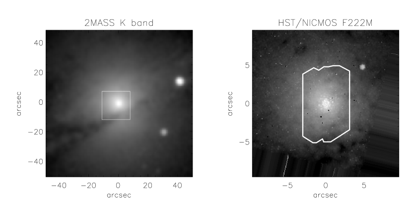
Figure 1: Broad band observations of central region of Cen A. Left: ground-based 2MASS K-band image; the over-plotted square shows the size and orientation of the right image. Right: HST/NICMOS F222M image with over-plotted footprint of the cirpass  field-of-view. On both images North is up and East to the left. HST image has been rotated accordingly.

3 Results

Our observations cover the nucleus of Cen A. The orientation and the size of the merged cirpass  field can be seen in Fig. 1. In this section we present the cirpass  data cube and compare it with other observations.

3.1 Nuclear spectrum

All spectra within a circular aperture of $0\aas@@fstack{\prime\prime}5$ radius were combined to form the nuclear spectrum presented on Fig. 2. There one can see the three major emission-lines which are of interest for this study. They are, in order of their observed relative strengths: [FeII] $\lambda$12567, Paschen $\beta$ $\lambda$12818 and [PII] $\lambda$11882 (Oliva et al., 1990). The observed lines are redshifted, with respect to their laboratory values, by 22 Å, corresponding to a velocity of 543 $\>{\rm km}\,{\rm s}^{-1}$. The first two lines were already observed by Marconi et al. (2001) having the ratio of $\sim 1.7$, but the observation of the [PII] line is, to our knowledge, the second extragalactic measurement of this emission-line, the first being in NGC 1068 by Oliva et al. (2001). The blue wings of the [FeII] and Pa$\beta$ emission-lines could be attributed to HeI $\lambda$12530 and HeI $\lambda$12790 emission. There is, however, no evidence for presence of HeI$\lambda 11970$ emission, which suggests HeI is generally not strong. The origin of the red wing of the [PII] is not known. The detected emission-lines are not contaminated by sky lines, except a minor contribution from the sky lines to the bluest part of the Pa$\beta$ wing.

Figure 2: Total spectrum from a circular aperture of $0\aas@@fstack{\prime\prime}5$ radius, centred on the nucleus. Three emission-lines used in this study are labelled at the wavelength redshifted for 543 $\>{\rm km}\,{\rm s}^{-1}$. The vertical dashed lines show the position of two candidate lines contributing to the blue wings of detected emission-lines. There is no evidence for existence of HeI$\lambda 11970$ line (dot-dashed line). The vertical lines at the bottom of the spectrum show positions of the sky lines in the observed wavelength region.

The relative strengths of the lines can be used to determine the nature of the ionisation mechanism. We estimated the strength of the emission by fitting double Gaussians (see Section 4.1 for more details) within apertures of increasing diameter, centred on the nucleus. Table 2 shows the measurement of the ratio of the lines. Within a 0$\aas@@fstack{\prime\prime}$25 aperture [FeII]/Pa$\beta\sim 2.3$, while [FeII]/[PII] $\sim 3.0$. As the aperture increases the [FeII]/Pa$\beta$ ratio fluctuates between 2.1 and 2.8, being typical of active galaxies or supernova remnants, as can be seen from observations and line diagnostic diagrams (e.g. Simpson et al., 1996; Alonso-Herrero et al., 1997; Mouri et al., 2000; Rodríguez-Ardila et al., 2004). The active nucleus in Cen A is an obvious source of [FeII] emission-lines, and although it is possible that a fraction of the [FeII]/Pa$\beta$ ratio is caused by star-formation (e.g. supernova remnants in the star forming regions), the fact that [FeII] emission is associated with shock, also points towards a mass outflow from the nucleus (e.g. the jet) and resulting shocks as the source of ionisation (Kawara et al., 1988).

The [FeII]/[PII] ratio, however, shows a clearly increasing trend, reaching 4.7 at the largest aperture. This can be used to asses the importance of shocks in the total ionisation mechanism of [FeII] lines. Oliva et al. (2001) found that the [FeII]/[PII] ratio is a good indicator for distinguishing the origin of the emission-lines, especially if they are ionised through photoionisation by soft X-rays or shocks propagating through the interstellar medium. The authors state that in regions with [FeII]/[PII] $\lesssim 2$ gas is photoionised, while if [FeII]/[PII] $\gtrsim 20$ the material is excited by collisions in fast shock waves. The observed values of the ratio are between these two limiting values, although closer to the upper limit for photoionisation, suggesting the AGN X-rays emission as the source of photoionisation. Still, the rising values argue that shocks play an increasingly important role in ionising the interstellar medium further away from the nucleus. This could be reflected in the motion of gas clouds, where a more settled motion should be observed in the central regions.

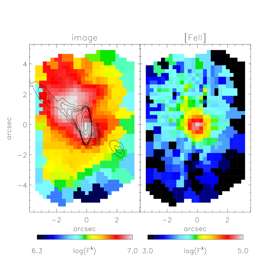
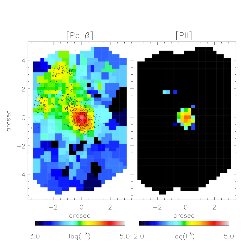
Figure 3: Maps obtained by summing the data cube along the spectral dimension after binning to $S/N=20$. The maps are oriented such that North is up and East to the left. From left to right: summed spectra with over-plotted VLA radio observations, spectra summed between 12554 - 12622 Å  ([FeII] line), spectra summed between 12807 - 12874 Å  (Pa $\beta$ line) with over-plotted Pa$\alpha$ emission from archival HST/NICOMS observations, spectra summed between 11870 - 11937 Å  ([PII] line). Note the change in the scale for the [PII] map, the agreement between Pa$\alpha$ and Pa$\beta$ structures and the coincidence of the N1 knot in the jet with the North-East flux peak in our observations. Flux $F^{\lambda}$ is in units of $10^{-17}$ ergs/s/m²/Å.

Table 2: Emission-line ratios within circular apertures of different sizes centred on the nucleus

$$\begin{array}[]{ccc}\hline\cr\vskip 3.0pt plus 1.0pt minus 1.0pt\cr$aperture$&$[FeII]/Pa$\beta&$[FeII]/[PII]$\\ (1)&(2)&(3)\\ \vskip 3.0pt plus 1.0pt minus 1.0pt\cr\hline\cr 0.25&2.3&3.0\\ 0.5&2.8&3.5\\ 0.75&2.1&3.7\\ 1.0&2.2&4.2\\ 1.25&2.6&4.7\\ \vskip 3.0pt plus 1.0pt minus 1.0pt\cr\hline\cr\end{array}$$

Notes – Col.(1): Radius of aperture [arcsec]; Col.(2): ratio of [FeII]/Pa$\beta$ flux Col.(3): ratio of [FeII]/[PII] flux.

3.2 Extent of the emission

Figure 3 presents the spatial extent of the J-band CIRPASS observations of Cen A. We binned the final merged data cube to an S/N of 20. The binned spectra were continuum subtracted after fitting 4th order polynomials to emission-free parts of spectra. The emission-lines presented in Fig. 3 were measured by summing the continuum subtracted spectra along the wavelength dimension in limited spectral regions centred on the lines themselves (see the caption of Fig. 3 caption for details).

Maps show two spatially separated regions of high integrated flux, one in the nucleus (for the determination of the central pixel see Section 3.3) and the other in the North-East region (NE), about 2″away from the nucleus. The detected emission-lines are mostly confined to the central $1\arcsec$, but Pa$\beta$ and [FeII] emission also extend towards the NE. Pa$\beta$ is also present in two blobs about 3″away from the nucleus. The weakest emission comes from [PII]. This emission-line falls off rapidly and outside 1″  the summed spectra are dominated by noise, but one can obtain information on somewhat larger radius (e.g. within 1$\aas@@fstack{\prime\prime}$25) by fitting the spectral line as done in Section 4.1.

3.3 Comparison with observations on different wavelengths

In order to determine the position of the nucleus in the CIRPASS data, we compared our observations with HST imaging. Schreier et al. (1998) identified the nucleus with the peak in Pa$\alpha$ emission, which also corresponds with the peak visible on K band (F222W) NICMOS images and the position of the radio nucleus. We find the position of Cen A’s nucleus in our observations by assuming that the Pa$\alpha$ and Pa$\beta$ emission have the same spatial origin and by cross-correlating the NICMOS F187N narrow band image with an image constructed from our unbinned data cube summed over the spectral region of the Pa$\beta$ emission.

The spatial distribution of the two Paschen lines matches well, as it can be seen in Fig. 3, where the NICMOS Pa$\alpha$ image is over-plotted on the binned Pa$\beta$ image. Schreier et al. (1998) determined the position angle of the elongation to be $\sim 33\degr$. Also, the two off centred blobs are well matched in this comparison. The extended distribution of Pa$\alpha$ emission is also traced by Pa$\beta$ emission.

We also compared the CIRPASS observation of Cen A with existing radio and X-ray observations (Hardcastle et al., 2003). Most of the action in the radio and X-ray happens at larger radii. This is especially the case for X-rays where the central region is featureless, and the very centre is saturated. The existence of X-rays, however, suggests a possible excitation mechanism for the observed spectral lines.

Radio observations trace a jet with a position angle of 51°(Clarke et al., 1992) down to the radio nucleus. Radio contours are over-plotted on a CIRPASS image obtained by summing all the spectra along the wavelength dimensions (Fig. 3). The direction of the radio jet coincides in projection with the NE region of high flux. The jet crosses the region of high flux loosing its energy: at the start of the region the energy in the jet is 10 mJy/beam and at the end the emitted energy is about 1 mJy/beam (the lowest plotted contour). This drop in jet’s intensity was used to define knot N1 by Burns et al. (1983). The direction of the jet is about 18°away from the orientation of the Schreier et al. (1998) Pa$\alpha$ disk, but between the two Pa$\beta$ (and Pa$\alpha$) blobs, touching the top of the East blob at the position of the kink in the jet. The kink in the jet could be explained as a deflection of the jet from a cloud complex which is now glowing in Pa$\beta$ light.

Figure 4: An example of two spectra, one from the North-East region of high continuum level (top spectrum) and the other from the opposite South-West region with typical a continuum level (bottom spectrum). The spatial coordinates are ($-1\arcsec$, $-1\aas@@fstack{\prime\prime}26$) and ($1\aas@@fstack{\prime\prime}1$, $-1\aas@@fstack{\prime\prime}7$), for top and bottom spectrum, respectively.

3.4 A hole in the extinction map or a jet-induced star formation region?

The most striking feature of the reconstructed images is the secondary peak in the integrated light which, in projection, is co-spatial with the radio jet, bounded by the two Pa$\beta$ blobs and arises at the end of knot N1. Cen A was the first object for which it was suggested that star formation in certain regions was jet-induced (Graham & Price, 1981; Brodie et al., 1983), soon followed by the Minkowski object (van Breugel et al., 1985), and numerous other objects with different environments and jet powers at low and high redshifts. The connection between the suggested nuclear star formation and the radio jet is, however, not as straight forward as at large scales, where blobs of optical emission and enhanced continuum correspond to specific jet structures. In this case, the end of a jet knot is followed by an increase in the total near-infrared flux, mostly coming from the continuum (in the same region there are no strong emission-lines), and bounded with regions of detectable emission: North and East Pa$\beta$ blobs and the nucleus. Interestingly, the East Pa$\beta$ blob coincides with the kink in the radio jet.

There are a few possible explanations for these observations. The two most likely are that the NE flux peak is related to a jet-induced star formation or that it coincides with the location of a hole in the extinction. In the first scenario, star formation could happen under the influence of the jet as it plows through the inter-stellar medium pushing gas clouds away from its path, and resulting in a region with higher stellar continuum. In the same time, Pa$\beta$ blobs could be ionised from the central engine or the jet, provided that they are on the unobscured path of non-thermal photons. In the second scenario, the NE flux peak is visible because it is under an extinction hole. In addition to that, the North and East Pa$\beta$ blobs may also originate in star forming regions where young stars provide enough photons to ionise gas clouds.

The extinction hole is supported by HST/WFPC2 F814W images (third panels on Figs. 5 and 8 of Marconi et al., 2000) on which the nucleus (a faint point source) and the less obscured NE region, which looks like a low extinction hole, are separated by a dust lane. The dereddend F814W image does not have similar features. The F222M image (K-band, presented on the same figures), which is less influenced by obscuring material shows only a marginal increase of flux in the NE region. The spectra from NE (high continuum) and SW (low continuum) regions are, however, very similar (Fig. 4), NE spectra being systematically higher, without any suggestion of change in the spectral slope, as it would be expected from regions of different extinction.

Assuming that jet induced star formation is the source of the high continuum and the Pa$\beta$ emission in the blobs, it is possible that the North Pa$\beta$ blob was also once induced by the jet (the jet is currently on the East Pa$\beta$ blob), which precessed down with time (in projection) from $PA=\sim 25\degr$ to present $PA=\sim 50\degr$.

It is hard from the present observations to disentangle the true origin of the properties of the North-East region. The precession of the jet is perhaps a far-fetched assumption, but our data, which are not complete enough for a decisive conclusion, support marginally more the jet-induced star formation in the continuum region, where an extinction hole can also contribute to the detection.

4 Kinematical properties of the nuclear disk

In the previous section we binned to a S/N ratio of 20 to present the data and discus the main trends. In this section we concentrate on the three observed emission-lines and use the A/N ratio based binning. We used a value of A/N = 2.5 for all three lines.

4.1 Narrow and broad components

The shape of the emission-lines on Fig 2 suggest that single Gaussians are not always adequate line models. Hence, we fitted the spectral features with double Gaussians when necessary. Each of the three emission-lines in a given spectrum were fitted separately and independently. Firstly, we fit the spectra with a 4th order polynomial avoiding the regions with the emission-lines. We subtract this continuum contribution and each emission-line we fit with a single Gaussian. These two fits are used as preparation steps for the final fit of the emission lines. In the final fit, we fit a double Gaussian and a 4th order polynomial simultaneously to the original spectra (not continuum subtracted). The parameters of the continuum fit and the single Gaussian fit are used as initial values in the minimisation procedure of the final fit. The results of the continuum fit were taken as the initial values of the 4th order polynomial parameters. The initial values of the double Gaussians parameters were chosen from the single Gaussian fit in the following way: (i) sigma (width) of the first Gaussian was set to be a half of the sigma of the single Gaussian fit; the sigma of the second Gaussian was kept the same as in the fit with the single Gaussian, and (ii) the mean of the first Gaussian was set to be equal to the mean obtained by the single Gaussian fit. The mean of the second Gaussian was set to be about 730 km/s (30 Å) less than the systemic velocity of the galaxy.

To robustly constrain the final fit we introduced the following limits for the parameters of the first Gaussian: (i) the mean was allowed to vary 250 km/s around the initial value, and (ii) the sigma was bounded between 4 and 15 Å(or 95 km/s and 350 km/s). The lower boundary is the instrumental resolution. The second Gaussian had the following constraints: (i) the mean was allowed to vary 500 km/s around the initial value, and (ii) the sigma was bounded between 4 and 45 Å(or 95 km/s and 1000 km/s). The upper boundary was seldomly reached. The final fit with a double Gaussian was performed using the MINPACK implementation (Moré et al., 1980) of the Levenberg-Marquardt least-square minimisation method. The double Gaussian system increased the goodness of fit, but it was not required at all positions for all emission-lines. The second Gaussian was needed to fit the Pa$\beta$ emission-line almost everywhere in the field while for [FeII] emission, it was necessary only in the centre, and for [PII] almost not at all.

Figure 5: Maps of total intensity and kinematics of detected ($A/N=3$) emission-lines. Left: Pa$\beta$; right: [FeII]. From top to bottom: the total flux of the emission, the mean velocity (centre of the Gaussian), the velocity dispersion ($\sigma$ of the Gaussian, without the contribution from the instrument dispersion). Over-plotted contours are the contours of the total flux. Different symbols relate to spectra in Fig. 6. Flux $F^{\lambda}$ is in units of $10^{-17}$ ergs/s/m²/Å. Regions without detected emission are shown in dark grey.

Errors on the parameters of the Gaussians (kinematics) were obtained through Monte Carlo simulations. For each double Gaussian fit to the data, we derived uncertainties from 100 random realisations of the best fit, where the value at each pixel is taken from a Gaussian distribution with the mean of the best fit and standard deviation measured on the residuals between the fit and the data. All realisations together provide a distribution of values from which we estimate $1\sigma$ (68.3%) uncertainties.

It is not necessary to expect that binning will always reach the set levels, since the emission need not to be present, and binning the noise will not create signal. Calculated amplitudes of both narrow and broad Gaussians and the standard deviation of the residuals of the fit can be used a posteriori to determine the true $A/N$ ratio of our data. Results show that the reached $A/N$ drops below the targeted level outside of the central region (size depends on the emission line). The quickest spatial drop in $A/N$ is seen for [PII], and the slowest for [FeII] emission-lines. Also, the highest $A/N$ is measured for [FeII] and the lowest in [PII] lines.

Sarzi et al. (2006) extensively discuss at which level of $A/N$ ratio an emission-line is robustly detected. This depends on the local spectral features (existence of complex absorption features will require a higher A/N ratio), but, generally, an emission-line with $A/N=2.5-3$ can be considered as detected. We binned to $A/N=2.5$ to keep the spatial resolution as high as possible, but in a posteriori check we chose a more conservative limit of $A/N=3$, and in the rest of the analysis we consider only emission-lines above this level.

Emission-lines that met the above criterion are presented in Figs. 5 and 6. The two rows of Fig. 5 show the two-dimensional extent, morphology and kinematics of Pa$\beta$ and [FeII] emission-lines, respectively from top to bottom. The [PII] emission-line reached $A/N=3$ level only in the central 0$\aas@@fstack{\prime\prime}$5 and the quality of the extracted kinematics was rather poor, so we do not consider it in the rest of the study. Fig. 6 shows examples of the spectral features obtained from the same spatial positions indicated by the symbols on both figures, but for different emission-lines (from top to bottom: Pa$\beta$ and [FeII], respectively).

Figure 6: Example of spectral features recovered from different positions in the nucleus of Cen A for different emission-lines. Top: Pa$\beta$; bottom: [FeII]. Symbols in top left corner are the same as symbols in Fig. 5. Every symbol shows the spatial location of the bin from which the spectrum was taken. Only regions around the given emission-line used in the fit are shown. Yellow, blue and light blue dashed lines are narrow, broad Gaussian components and the fit to the continuum, respectively. The red line shows the combined fit to the data. Note the strong contribution of the broad Gaussian to the central Pa$\beta$ emission. Error bars ($1\sigma$) are plotted for every 10th data point for clarity.

Although at almost all positions a combination of a narrow and a broad Gaussian is required to fit the Pa$\beta$ emission-line, only in a few cases the broad component can be really recognised as a separate line. More often, the broad component serves as an additional continuum correction (Fig. 6). When present, the broad Gaussians are blue shifted with respect to the narrow Gaussians for (always) $795\>{\rm km}\,{\rm s}^{-1}$. The spatial distribution of the broad component (with A/N $>3$) is limited and concentrated in the very centre and somewhat elongated in the NE direction, near the position of the jet and between the blobs of the narrow component. Line widths are generally less than $800\>{\rm km}\,{\rm s}^{-1}$ (sigma of the Gaussian), and as such are not comparable to the emission from classical broad-line regions in AGNs. We call this component broad only to distinguish it from the main line emission and we do not consider it further. The main (narrow) component is detected on a larger area in the centre and at the position of the Pa$\alpha$ blobs, (Fig. 3). Spatially, the distribution of the narrow Gaussians seems to be elongated along the NE direction with $PA\sim 30\degr$. This value is consistent with the position angle of Schreier et al. (1998) Pa$\alpha$ disk.

Different results are recovered from the [FeII] line. The broad Gaussian component to the [FeII] emission-line is almost completely absent, as expected for a forbidden line, except in the very centre where A/N is still below 3 and broad Gaussians improve the fit to the continuum more than fit a real (robust) emission feature (Fig. 6). The [FeII] line is detectable on a larger area than Pa$\beta$ and it is not elongated, but more circularly distributed. The emission is concentrated in the centre, but also spread towards the NE corner, approximately following the position of the jet, although it is just above the detection limit and patchy distributed, mostly over the East Pa$\beta$ blob and approaching the position of the North blob.

4.2 Kinematical evidence for a disk

Both Pa$\beta$ and [FeII] emission-lines show rotation and they are likely part of the nuclear disk structure discovered by Schreier et al. (1998). Here, we wish to describe their kinematic properties as they are given on Fig. 5.

The there regions with measured Pa$\beta$ emission (the centre, the East and the North blob), although spatially separated, seem to be part of the same kinematic structure. The central blob (covering roughly the central 1 arcsec²) shows a quite regular rotation, with zero-velocity curve (ZVC) lying horizontally in the East – West (EW) direction. The East blob is predominantly blue-shifted, while the North blob is red-shifted, with respect to the systemic velocity (the median velocity across the map is $\sim 560\>{\rm km}\,{\rm s}^{-1}$). All three blobs have similar velocity amplitudes and there is a clear division on the map: North is receding and the South(-East) is approaching the observer. If the emission were detected at all positions, it is likely that we could see a continuous kinematic map, with a twisting ZVC: from horizontal (EW direction) to almost $45\degr$ (NE-SW direction).

Velocity dispersions, measured as the width ($\sigma$) of the narrow component Gaussian, confirm the relations between the blobs. The East and North blob have low velocity dispersion as well as the outer regions of the central blob. The dispersion increases towards the centre (staying below $200\>{\rm km}\,{\rm s}^{-1}$), possibly being elongated perpendicular to the orientation of the central blob ($PA\sim-60\degr$). The low velocity dispersion over most of the region also suggests a regularly rotating structure, such as a thin disk of gas clouds.

[FeII] emission covers a larger area and it fills some of the gaps seen on the Pa$\beta$ maps. The distribution of velocities is remarkably similar between the two lines. [FeII] emission also shows rotation (the median velocity across the map is $\sim 590\>{\rm km}\,{\rm s}^{-1}$), which changes direction: the ZVC is oriented E-W in the centre, but beyond 1″  it twists towards NE-SW. Actually, the ZVCs on Pa$\beta$ and [FeII] maps have identical spatial positions and orientations, where the North on [FeII] map is receding and the South is approaching. Beyond 2″where the emission becomes patchy, it is still possible to trace the rotation of the whole structure.

The velocity dispersion is low in the outer regions, but rises towards the centre. It is higher than the Pa$\beta$ velocity dispersion everywhere, except at the edges of the detection region. It also rises faster (median level is $\sim 127\>{\rm km}\,{\rm s}^{-1}$), until levelling at a plateau ($\sim 200\>{\rm km}\,{\rm s}^{-1}$) which is elongated in the same directions as the enhanced Pa$\beta$ velocity dispersion structure. The orientation of the plateau ($PA=-60\degr$) is unexpected also because it is not aligned with the the ZVC. An increase along the ZVC could come from unresolved rotation in the steepest part of the velocity map (where velocities change from approaching to receding), but even in this extreme case the velocity dispersion would not be as elongated. We will follow this issue further in Sections 4.3 and 5.3.

From Fig. 5 it is obvious that different blobs of Pa$\beta$ and [FeII] emission have related kinematics, even when they are spatially separated. A similar finding is also visible on SAURON maps of ionised gas in early-type galaxies (Sarzi et al., 2006) and bulges of Sa galaxies (Falcón-Barroso et al., 2006), where gas although patchy or along filaments shows continuous kinematics, suggesting that all emission elements belong to the same dynamical structure, but that the level of ionisation, the amount of gas or extinction is not the same and varies locally.

The rotation of both lines is to a first order regular and suggests that the emission is distributed in a disk-like structure. It is also clear that the kinematics of Pa$\beta$ and [FeII] emission are generally similar (velocity orientation and amplitude), but there are some notable differences such as a higher velocity dispersion in [FeII] lines. Judging from velocity dispersion maps, it seems that [FeII] emission is more perturbed than Pa$\beta$ and its motion is not completely ordered nor purely disk-like. Deviations could be caused by physical processes such as inflows, outflows, non-axisymmetric perturbations in the potential, warps or simply material not belonging to the disk. We investigate this in more details below.

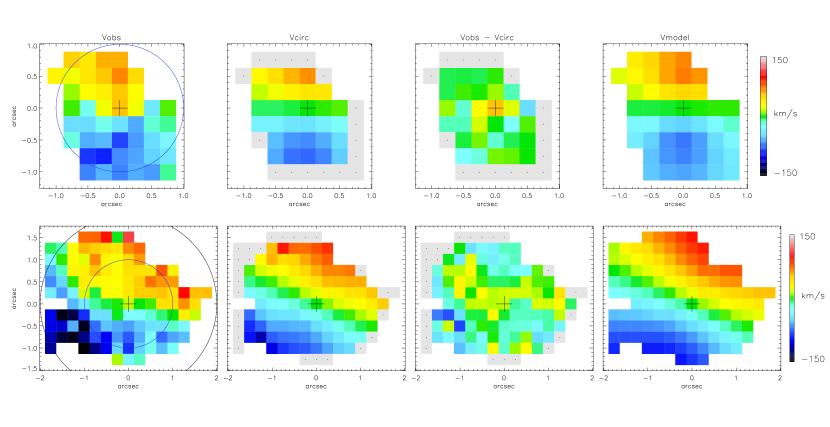
Figure 7: Maps of the observed mean velocity (far left), circular velocity (middle left), residuals between the mean and circular velocity (middle right), and the best fitting thin disk models (far right) using the derived orientation for Pa$\beta$ (top) and [FeII] (bottom) emission-lines disks. Circles over-plotted on observed velocity maps have radii of 0$\aas@@fstack{\prime\prime}$9 (blue) and 1$\aas@@fstack{\prime\prime}$8 (black). Bins marked with black dots were not included when constructing circular velocity maps. The plus symbol denotes the origin of the map, assumed to be the position of the Cen A nucleus. Standard deviations of residual maps are $18\>{\rm km}\,{\rm s}^{-1}$ and $25\>{\rm km}\,{\rm s}^{-1}$ (but $16\>{\rm km}\,{\rm s}^{-1}$ within the blue circle), for Pa$\beta$ and [FeII] maps, respectively. The method to construct circular velocity maps is described in Section 4.3 and the thin disk model is described in Section 5.

4.3 Orientation of the velocity structures

Assuming that the velocities represent material moving in a thin disk, it is, in principle, possible to determine both $PA$ and inclination ($i$) at the same time and as a function of radius. This is, in practice, often quite difficult, especially if there are deviations from circular rotation or data are noisy. In our case, we decided to determine only global properties and to do that through a two stage process.

We first follow the method for determination of the global kinematic $PA$ from Appendix C of Krajnović et al. (2006). Briefly, one constructs a set of bi-anti-symmetric velocity maps (because of the assumed axisymmetry) with different $PAs$ and compare them with the observed velocity map. The likeness of a model map ($V_{m}$) to the observed map ($V$) is measured by the quantity $\chi^{2}=\sum^{N}_{j}[(V_{m,j}-V_{j})/\Delta V_{j}]^{2}$, where $\Delta V_{j}$ are measurement errors on velocities for each bin $j$ on a map $m$. The model map with the $PA$ closest to the observed value will contribute with the smallest $\chi^{2}$.

We applied this method to [FeII] and Pa$\beta$ maps which were slightly modified by selecting only spatially continuous emission on the maps. This meant decreasing the size of maps to the central regions (about 1 arcsec² for Pa$\beta$ and about 2 arcsec² for [FeII]), but increased the robustness of the method. For these trimmed maps (see the first column in Fig. 7) we obtained the following values: $PA=-3\degr\pm 10\degr$ for Pa$\beta$ and $PA=-23\degr\pm 3\degr$ for [FeII] velocity maps. All errors quoted here are at $3\sigma$ confidence level. The [FeII] map is about 2 times larger than the Pa$\beta$ map and difference in $PA$ comes from the change in the ZVC as one includes a larger area. On Fig. 7 the blue and black circles on the maps show the regions used in the fit to determine the $PA$ for Pa$\beta$ and [FeII], respectively. Repeating the exercise for [FeII] within the blue circle, one gets $PA=-14\degr\pm 5\degr$, which is in good agreement with the Pa$\beta$ value.

The next step is to estimate the inclination of the disk assuming that the motion in the disk is purely circular. In that case, a velocity profile extracted along an ellipse will be described by a cosine law, if the ellipse samples equal radii in the disk plane and has the same $PA$ as the disk. This ellipse is then related to the inclination through its ellipticity: $1-\epsilon=\cos i$. Using the kinemetry software of Krajnović et al. (2006) and assuming a constant $PA$ measured above, we estimate the $i$ of the maps in the following way. Starting from a given $i$ we stepped through the velocity map extracting velocity profiles along ellipses with $1-\epsilon=\cos i$ and increasing semi-major axis $R$. Each velocity profile we least-squares fitted with the formula $V(R,\theta)=(V_{c}(R)/\sin i)\cos\theta$, where $V_{c}$ is the circular velocity and $\theta$ eccentric anomaly, measured from the projected major axis of the ellipse (given by the fixed $PA$). We linearly interpolated $V(R,\theta)$ to $V(x,y)$ creating a model velocity map at the observed coordinates on the sky. This has been done for a range of different inclinations and each model velocity map ($V_{m}$) was compared to the observed map ($V$) similarly as above using a quantity: $\chi^{2}=\sum^{N}_{j}[(V_{m,j}-V_{j})/\Delta V_{j}]^{2}$, where $\Delta V$ are measurement errors. The inclination of the model map with the minimum $\chi^{2}$ was recognised as the global estimate of the inclination of the observed disk. An almost identical procedure (they varied both $PA$ and $i$ simultaneously) was used previously by Buson et al. (2006).

In the case of Pa$\beta$ emission, setting the $PA$ to $-3\degr$ we obtained $i=25\degr\pm 5\degr$. Setting the $PA$ to $-23\degr$ for [FeII] disk we obtained $i=30\degr\pm 5\degr$. The two inclinations are consistent with each other, and are also consistent with studies (Marconi et al. (2001), Silge et al. (2005), Marconi et al. (2006)), but somewhat smaller than models by (Häring-Neumayer et al., 2006). In the second column of Fig. 7 we show the reconstructed circular velocity maps using the best fitting $PA$ and $i$.

Figure 8: Measured emission-line velocities and model predictions (see Section 5 for details) along $PA=0\degr$. The [FeII] velocity data and the best fitting model are shown with triangles and the dashed-dotted line, respectively. The Pa$\beta$ velocity data and the best fitting model are shown with filled circles and the black line.

One can most clearly see the deviations from a pure circular motion on the residual maps obtained by subtracting the reconstructed circular velocity maps from the observed velocities (shown in column 3 on Fig. 7). Both residual maps have visible non-zero components. On average, residuals are higher on the [FeII] map (standard deviation is $18\>{\rm km}\,{\rm s}^{-1}$ for Pa$\beta$ and $25\>{\rm km}\,{\rm s}^{-1}$ for [FeII]), but within the central region (blue circle) the residual are very similar and have the same spatial trend )standard deviation of $\sim 16\>{\rm km}\,{\rm s}^{-1}$). This is consistent with the rising [FeII]/[PII] ratio towards the edge of the map, where shocks become an increasingly important factor in the ionisation mechanism, and possibly influence the kinematics. Shocks can result from the jet interaction with the surrounding matter, but can also occur between the tilted rings of the warped disk. On larger scales ([FeII] residuals map) there is a hint of a more complicated pattern which primarily arises from the difference between the observed (changing) and assumed (constant) orientation. This, possibly three-fold, pattern can be associated with inflows, outflows or warps.

The most distinct feature on the velocity maps is the twist of the ZVC beyond 1″. Inside this radii the black hole is dominating the potential (Marconi et al., 2006) and is able to stabilise gas clouds in a disk. The central blob of Pa$\beta$ emission is largely confined to this region only, but iron is ionised in almost continuous gas clouds up to 2″, and the influence of instabilities is visible in the central emission-line disk. The two other Pa$\beta$ blobs at $~{}\sim 2.5\arcsec-3\arcsec$ from the nuclei, behave similarly like [FeII] disk on large radii, being far from the sphere of influence of the black hole where the instability can perturb the disk.

The dusty disk in Cen A is known to be warped at kpc scales (Bland et al., 1987; Quillen et al., 1992; Nicholson et al., 1992; Quillen et al., 1993). There are evidences for a bar spiral system (Mirabel et al., 1999; Block & Sauvage, 2000; Leeuw et al., 2002), although the recent infrared observations support the warp disk hypothesis (Quillen et al., 2006). Our data shows that the warp (or a bar-like perturbation) can be traced all the way to 20 pc scales. It is, however, difficult to be conclusive on the matter from these data, and the meaning of residuals has to be taken with care, especially when the measured uncertainties are taken into account: $16\>{\rm km}\,{\rm s}^{-1}$ for Pa$\beta$ and $19\>{\rm km}\,{\rm s}^{-1}$ for [FeII]. We will, however, following the recent results, continue in the framework of the warped disk.

Comparing the orientation and the extent of the velocity dispersion plateau with the tilted ring model of Nicholson et al. (1992) and Quillen et al. (2006), we suggest that the origin of the high velocity dispersion is in the unresolved rotation coming from different folds of the warped disk. We draw this conclusion from Figs. 10 and 11 of Nicholson et al. (1992) and Figs. 5 and 7 of Quillen et al. (2006), which show that the disk changes its orientation such that in the inner part of the disk ($r<60\arcsec$) its SW points and in the outer part ($r>100\arcsec$) its NE points are closest to the observer. Although both studies construct the warped disk model to larger radii (beyond 40″) than what we present in this work, the orientation of the high velocity dispersion plateau ($PA=-60\degr$ or $PA=120\degr$) agrees well with the measured orientation of the warped disk. This means that our line-of-sight crosses the disk a few (at least two) times, and the observed kinematics will depend on where the ionisation of the gas clouds occurs.

The [Fe II] emission-line arises from partially ionised regions, i.e. regions with a few per cent fraction of HI in the HII state. These regions are typically seen in the narrow line region environment of an AGN, where X-ray photons from the central engine can penetrate deep into the cloud. Thus, partially ionised regions do not have a direct view of the central engine, being shielded by a column of $\sim 10^{20}$ cm^-2 of $N_{H}$. The observed [FeII] emission could originate in different folds of the warped disk, also further away from the central engine. The resulting large difference in velocities along the line-of-sight, observed as unresolved rotation, has two effects: the velocity gradient is shallower and the velocity dispersion higher than in the case of resolved rotation.

In Fig. 8 we compare the central velocity gradient between the Pa$\beta$ and [FeII] emission-lines, extracted from velocity maps along a slit of 3″  length, 0$\aas@@fstack{\prime\prime}$25 width and $PA=0\degr$. Within $0\aas@@fstack{\prime\prime}5$, Pa$\beta$ emission shows a steeper rotation curve than [FeII] emission, while around 1″  both emission-lines reach the same level. In the substantially warped gas disk, the innermost regions would provide the required shielding for the [FeII] emitting material slightly further out. The lack of [FeII] emission from the innermost region, in contrast to Pa$\beta$, would explain a slower rise of the [Fe II] line-of-sight velocity curve with increasing radius, plotted in Fig. 8. Also, unlike Pa$\beta$, the [FeII] emitting material is confined to specific regions of the gas disk, increasing the likelihood that it provides an incomplete picture of the gas kinematics in the central region. The higher velocity dispersion indicate a more turbulent medium, one in which shocks may be playing an important role. This too, raises doubts about the [FeII] emitting gas serving as a good tracer of the gravitational potential in the innermost nuclear regions.

5 Evidence for the central black hole

In the previous section we showed evidence that the observed ionised gas is moving in a disk-like structure, which is consistent with being warped beyond 1″. In this region, the motion is not completely ordered, but the level of the residuals is comparable with measurement uncertainties. We also showed that [FeII] emission-line kinematics suffers from observed unresolved rotation, which can be explained with warped disk morphology. We continue the analysis by constructing simple dynamical models, based on the observed properties of the disk (orientation, circular motion) with a purpose of testing the hypothesis that there is a central black hole in Cen A that can explain the observed kinematics.

5.1 Mass models

As reported by Silge et al. (2005), the enclosed stellar mass within the central 1″  is $3\times 10^{7}M_{\odot}$, for a deredened profile, and $2\times 10^{7}M_{\odot}$ for an observed (not deredened) light profile. The mass of the black hole expected from the M${}_{\bullet}-\sigma$ relation (as given by Tremaine et al., 2002) is $3\times 10^{7}M_{\odot}$. The mass of the central black hole in Cen A determined by previous studies is, however, around $1\times 10^{8}M_{\odot}$. Assuming a velocity dispersion of $\sim 150\>{\rm km}\,{\rm s}^{-1}$ (Silge et al., 2005), the sphere of influence of this object is $\sim 1\aas@@fstack{\prime\prime}3$. This suggest that within 1″  the dominant contribution to the potential comes mostly from the central black hole. The total potential can then be written in the following way:

$$\Phi=\Phi_{\star}+\Phi_{\bullet},$$ (2)

where the black hole contribution is simply given by $\Phi_{\bullet}=GM_{\bullet}/r$, while $\Phi_{\star}$ can be derived from the stellar luminosity density assuming a mass-to-light ratio $M/L$. The stellar luminosity density of a system is obtained by deprojecting the observed surface brightness distribution, assuming a symmetry type (e.g. axisymmetry) for the system and its inclination. This can be conveniently done using the the Multi-Gaussian expansion method (MGE; Monnet et al., 1992; Emsellem et al., 1994).

Using the MGE software of Cappellari (2002), we simultaneously fitted a ground-based K-band image from 2MASS Large Galaxy Atlas (Jarrett et al., 2003) ( 3″$<$ r $<$ 200″) and the space-based NICMOS F222M image (Schreier et al., 1998) (0″$<$ r $<$ 9″). The 2MASS image was scaled to the NICMOS image, while the sky was measured on the 2MASS image. The MGE software analytically deconvolves the instrumental PSF from the observed light, which we determined using the TinyTim software Krist & Hook (2001) and also parameterised by three two-dimensional Gaussians, normalised such that their amplitudes, $G_{j}$, add up to unity. Following the suggestion in Cappellari (2002), we increased the minimal axial ratio of the Gaussians, $q_{j}$, while not changing $\chi^{2}$ significantly, in order to make as large as possible the range of permitted inclinations. Parameters describing the parametrisation of the PSF and the deconvolved MGE model are presented in Tables 3 and 4, while a comparison of the combined ground and space-based light profiles and the MGE model is shown in Fig. 9.

Figure 9: Comparison between the combined NICMOS/F222M and 2MASS K-band photometry (open squares) with the MGE model (line) in seven angular sections as a function of radius. The right panels show the radial variation of the relative error along the profiles.

Table 3: The MGE parameters of the circular PSF.

$$\begin{array}[]{ccc}\hline\cr\vskip 3.0pt plus 1.0pt minus 1.0pt\cr$j$&$G$_{j}&\sigma_{j}$(arcsec)$\\ \vskip 3.0pt plus 1.0pt minus 1.0pt\cr\hline\cr 1&0.754&0.041\\ 2&0.166&0.126\\ 3&0.080&0.508\\ \vskip 3.0pt plus 1.0pt minus 1.0pt\cr\hline\cr\end{array}$$

Table 4: The parameters of the MGE model of the deconvolved K-band surface brightness of Cen A.

$$\begin{array}[]{ccccc}\hline\cr\vskip 3.0pt plus 1.0pt minus 1.0pt\cr$j$&$I$_{j}(L_{\odot}{pc}^{-2})&\sigma_{j}$(arcsec)$&$q$_{j}&$L$_{j}(\times 10^{9}L_{\odot})\\ \vskip 3.0pt plus 1.0pt minus 1.0pt\cr\hline\cr 1&70122.1720&0.0506&0.9500&0.00030887\\ 2&113639.0196&0.4428&1.0000&0.040313\\ 3&68662.2409&1.2923&1.0000&0.20744\\ 4&56428.6385&2.9233&1.0000&0.87241\\ 5&34809.6545&5.3776&1.0000&1.8211\\ 6&19386.9662&13.6883&0.9500&6.2431\\ 7&7184.3315&37.4720&1.0000&18.250\\ 8&3174.4729&92.0318&0.9823&47.783\\ \vskip 3.0pt plus 1.0pt minus 1.0pt\cr\hline\cr\end{array}$$

5.2 Simple dynamical models

The basic assumption of our simple dynamical models is that clouds of ionised gas move in circular orbits within a thin disk. This is an often used approach pioneered for black hole studies by Macchetto et al. (1997) and subsequently applied to the ionised gas disk in Cen A by other authors (Marconi et al., 2001; Marconi et al., 2006; Häring-Neumayer et al., 2006).

The circular velocity is given by $V_{c}(R)=\sqrt{R(\mathrm{d}\Phi/\mathrm{d}R)}$, where the gravitational potential $\Phi$ is as in eq. (2). If mass-to-light ratio M/L is taken to be zero, the gravitational potential is described only by a ’point-mass’ contribution ($\Phi_{\bullet}$), and the circular velocity simplifies to $V_{c}(R)=\sqrt{GM_{\bullet}/R}$. This model we call Kepler, while the more complex model, which includes the contribution of the stellar potential we call MGE. The calculation of the potential from the MGE parametrisation in that case is done as described in Cappellari et al. (2002).

Thin disk models assume that the motion is purely circular and that the velocity dispersion of the gas is negligible. Our observations of the Pa$\beta$ disk are consistent with this assumption, but it breaks in the case of the [FeII] disk. We speculate that the increase in the velocity dispersion is related to the location of the [FeII] emission in the disk, the geometry of the warped disk and the turbulent medium with increasingly important [FeII] ionising shocks waves (see Section 5.3 for details). From this reasons, our observations of [FeII] emission are not good tracers of the central potential and are not suitable for the determination of the black hole mass with the presented dynamical models. In what follows, we focus only on the Pa$\beta$ emission, but we also construct a model for the [FeII] disk for comparison with observations (Figs 7 and 8).

To accurately reproduce the observed kinematics we include in the model the parametrisation of the emission-line surface brightness obtained by fitting a function to the measured flux, taking the $PA$ and the $i$ of the gas disk into account. We tested different functional forms, finally choosing the following one which describes the spatial distribution of the emission-lines surface brightness well:

$$I=I_{0}+I_{1}\exp{-\frac{r}{r_{1}}},$$ (3)

where $r_{1}$ is the scale radius and $I_{0}$ and $I_{1}$ are the scale factors for the given gas component. The best fitting values for the Pa$\beta$ assuming for the orientation of the disk ($PA=-3\degr,i=25\degr$) are $I_{0}=1844.4$, $I_{1}=32884.9$ and $r_{1}=0\aas@@fstack{\prime\prime}503$. For other orientations we obtain slightly different values and use those in the corresponding dynamical models.

When constructing dynamical models, we fix the geometry of the disk, use the above mentioned emission-line surface brightness parametrisation, and vary parameters defining the gravitational potential: M/L ratio and $M_{\bullet}$. The resulting models of the circular velocity maps, convolved with the PSF and the pixel size of the CIRAPSS observations (Qian et al., 1995), are compared with the observed models. The best fitting model is determined by minimising the $\chi^{2}=\sum^{N}_{j}[(V_{m,j}-V_{j})/\Delta V_{j}]^{2}$, similarly as done before.

Table 5: The parameters of the best fit thin disk models

$$\begin{array}[]{ccccccc}\hline\cr\vskip 3.0pt plus 1.0pt minus 1.0pt\cr$model$&$mass$&$i$&$PA $&M_{BH}&$M/L$&\chi^{2}\\ &$model$&$[degr]$&$[degr]$&$[$10^{7}$M$_{\bullet}$]$&$[K band]$&\\ \vskip 3.0pt plus 1.0pt minus 1.0pt\cr\hline\cr$Pa$\beta\\ \hline\cr\vskip 3.0pt plus 1.0pt minus 1.0pt\cr p1&$MGE$&25&-3&8.25^{+2.25}_{-4.25}&0.0+1.3&33.5\\ p2&$MGE$&30&-23&6.5^{+3.5}_{-2.5}&0.45^{+1.0}_{-0.45}&77.0\\ p3&$MGE$&25&-15&9.0^{+3.5}_{-3.0}&0.15^{+1.55}_{-0.15}&46.9\\ p4&$MGE$&45&-27&3.5^{+2.0}_{-2.5}&0.35^{+0.85}_{-0.35}&104.3\\ p5&$Kepler$&25&-3&8.25^{+2.00}_{-1.75}&0.0&33.5\\ p6&$Kepler$&30&-23&8.0^{+2.0}_{-2.0}&0.0&78.1\\ p7&$Kepler$&25&-15&9.5^{+2.0}_{-1.0}&0.0&47.0\\ p8&$Kepler$&45&-27&5.0^{+1.3}_{-1.0}&0.0&107.9\\ \vskip 3.0pt plus 1.0pt minus 1.0pt\cr\hline\cr\end{array}$$

Notes – We used two mass models: Kepler where the potential is given by the central point-mass, a mass model obtained from our MGE parametrisation of the stellar light. There were 47 velocity data points used to constrain the models.

Figure 10: A grid of models with different mass of the black hole ($M_{BH}$) and mass-to-light ratio ($M/L$) for the Pa$\beta$ disk at $i=25\degr$ and $PA=-3\degr$. Over-plotted are the contours of the constant $\chi^{2}$. The first three contours correspond to 68.3%, 95.4% and 99.73% (thick contour) confidence regions for a distribution of 2 degrees of freedom. The best fitting model is shown with a diamond.

5.3 Results and discussion

We calculated a range of dynamical models with different disk orientations, black hole masses and mass-to-light ratios. We applied the disk orientation from Section 4.3 for Pa$\beta$ emission-line disk and also used values from the literature (Marconi et al., 2006; Häring-Neumayer et al., 2006).

Table 5 presents the values of the best fitting models. Our best fitting orientation of the Pa$\beta$ disk yields a model with $M_{\bullet}=(8.25^{+2.25}_{-4.25})\times 10^{7}M_{\odot}$ and $M/L=0.0\pm 1.3$. Uncertainties quoted for all presented models are at the $3\sigma$ level. The expected value of $M_{\bullet}$ from the $M_{\bullet}-\sigma$ relation is excluded at a $3\sigma$ confidence level, taking into account the scatter of the relation of 0.34 dex (Ferrarese & Ford, 2005), but our estimate, within its large uncertainties, is consistent with other measurements in the literature at similar inclinations (Marconi et al., 2006; Häring-Neumayer et al., 2006). Values for $M_{\bullet}$ obtained from stellar kinematics (Silge et al., 2005) are still higher (even their model for $i=20\degr$) and formally excluded at a $3\sigma$ level. The estimated $M/L$ ratio of the best fitting model is consistent with being zero confirming that within 1″  the gravitational potential is almost entirely determined by the black hole and not dependant much on the parametrisation of the stellar light.

Confidence levels over-plotted on the grid of different models with our best fitting disk orientation are presented in Fig. 10. The reconstructed velocity map of the best model is shown in Fig. 7 and a cut along $PA=0\degr$ in Fig. 8. For completeness, we report here that using our best fitting orientation for the [FeII] disk we get $M_{BH}=(0.1^{+1.0}_{-0.1})\times 10^{7}M_{\bullet}$ and $M/L=2.0\pm 0.4$. The untrustworthiness of this model can be seen in Figs. 7 (last panel) and 8 (dash-dotted line).

In the construction of the thin disk models the orientation of the disk is crucial, and the final parameters of the potential ($M_{\bullet}$, $M/L$) will depend on it. We constructed other dynamical models (Table 5) using a set of disk geometries. For Pa$\beta$: the best orientation obtained from [FeII] kinematics (model p2), the best disk orientation from Marconi et al. (2006) (model p3) and geometry of the best model from Häring-Neumayer et al. (2006) (model p4). Model p5 has the best Pa$\beta$ disk geometry obtained from the kinematics, while models p6 – p8 have the same geometries as above (in the same order), but these mass models include only the contribution from the black hole.

In the last column of Table 5, $\chi^{2}$ values for each model are listed. The best model is p1, with a geometry determined from the kinematics derived in Section 4.3. Models p1 and p5 are formally equally good, but other models (including p3 and p7) are excluded at the $3\sigma$ level (for 2D distribution). The models are more sensitive to the inclination than to a change in $PA$. Models with Keplerian and MGE mass parametrisation give similar results, but the uncertainties in the estimated mass are somewhat smaller in Keplerian models, which have a fixed M/L.

As an additional check of our results, we also constructed models with a given $M_{\bullet}$ and $M/L$ with the purpose to recover the measured disk orientations( $PA$, $i$). We chose models with parameters from the literature: Häring-Neumayer et al. (2006) – model pg1, Marconi et al. (2006) – model pg2, Silge et al. (2005) – model pg3. The models pg4 is a hybrid combining the value from the M${}_{\bullet}-\sigma$ relation and the $M/L$ ratio from other studies. Results are given in Table 6.

Table 6: Additional disk models for given M_∙ and $M/L$ ratio.

$$\begin{array}[]{ccccccc}\hline\cr\vskip 3.0pt plus 1.0pt minus 1.0pt\cr$model$&$mass$&M_{BH}&$M/L$&$i$&$PA $&\chi^{2}\\ &$model$&$[$10^{7}$M$_{\bullet}$]$&$[K band]$&$[degr]$&$[degr]$&\\ \vskip 3.0pt plus 1.0pt minus 1.0pt\cr\hline\cr$Pa$\beta\\ \hline\cr\vskip 3.0pt plus 1.0pt minus 1.0pt\cr pg1&$MGE$&6.1&0.7&25\pm 5&-5^{+10}_{-10}&37.3\\ pg2&$MGE$&11.0&0.0&20\pm 5&0^{+9}_{-13}&34.6\\ pg3&$MGE$&24.0&0.68&20\pm 1&-20^{+7}_{-6}&128.6\\ pg4&$MGE$&3.0&0.7&30^{+10}_{-7}&0^{+7}_{-15}&44.4\\ \vskip 3.0pt plus 1.0pt minus 1.0pt\cr\hline\cr\end{array}$$

As with previous models, most configurations give similar goodness of fit values, only model pg3 has a very different $\chi^{2}$ and can be discarded. All models recover mutually consistent (within errors) geometrical parameters which are also in good agreement with values obtained in Section 4.3. Model pg2 (Marconi et al. (2006) geometry) is expectedly the closest to our best fitting model (p1) in terms of $\chi^{2}$. Assuming M_∙ from the Tremaine et al. (2002) relation gives a model that is close to be discarded with $3\sigma$ confidence level.

6 Conclusions

This paper presents observations of the active elliptical galaxy, NGC 5128 (Cen A), obtained with the integral-field spectrograph cirpass. In the spectra there are three emission-lines, [PII], [FeII] and Pa$\beta$, with different spatial distributions and relative strengths. All lines are present in the central 1″, [FeII] being the most extended. Pa$\beta$ is also detected in two blobs, North and East of the nucleus. These blobs are in an excellent agreement with Pa$\alpha$ blobs discovered by the HST imaging. Analysis and results are summarised in the following items.

• The reconstructed total intensity image shows two regions with strong continuum contribution: in the centre and NE of the centre. The NE region overlaps with the position of the radio jet (in projection) and is located between the Pa$\beta$ blobs. The region can also be associated with the knot N1 of the radio jet. This suggests a possible jet-induced star forming region in Cen A on scales of $\sim 30$ pc, in addition to the well known large scale (1kpc) jet-induced star forming region.

• The location of the East Pa$\beta$ blob coincides with the kink in the radio jet suggesting a direct link between the two phenomena. If one assumes that the North Pa$\beta$ blob was also induced by the jet, the position of the blobs show that the jet precessed for about 25°in projection.

• We detect [PII] emission, which can be used together with [FeII] emission to discriminate between photo- and shock-induced ionisation of gas clouds. The [FeII]/[PII] ratio rises steadily with radius, being close, but above pure photo-ionisation levels. This suggests that shocks are more important with increasing distance from the centre.

• We determined spatially resolved kinematics from Pa$\beta$ and [FeII] emission-lines. Although the emission (of both lines) is divided in blobs or it is patchy at certain regions, it has a well defined and uniform sense of rotation and spatially separated emission regions are part of the same kinematic structure. The velocity dispersion is low for Pa$\beta$, but high for [FeII] emission with a plateau oriented at $\sim-60\degr$. The low dispersion is suggestive of a motion in a regular disk for Pa$\beta$, but the plateau in the [FeII] velocity dispersion is a clear evidence of a more complex distribution of ionised iron.

• Kinematics of both emission-lines is remarkably similar in appearance, as traced by ZVC: central regions are rotating around an EW axis, while at larger radii there is a twist in ZVC and the rotation is around NE – SW axis. The twist in ZVC suggest contribution from a bar-like perturbation or a warp in the disk on 20 pc scales.

• We test the assumption that the emission in the central 1-2″  is confined to a disk by constructing maps of circular velocity and comparing them with observations. This process is divided in two steps. We first determine the $PA$ and (using this position angle) the inclination of the assumed disk. The best fitting parameters are: $PA=-3\degr\pm 10\degr$ and $i=25\degr\pm 5$ for Pa$\beta$ and $PA=-23\degr\pm 3\degr$ and $i=30\degr\pm 5$ for [FeII]. Using these values we extract circular velocity component and remove it from the data. The residual map of Pa$\beta$ velocities is noisy without recognisable pattern and residuals are largely within measurement errors. [FeII] residuals are more complicated, showing a three-fold pattern and being somewhat larger than measurement uncertainties. This can be traced to the twist in the ZVC. We conclude that the emission in the central 1″, the region which is likely to be within the sphere of influence of the central black hole, is consistent with being in circular motion in a disk, but outer regions show departures which could be attributed to perturbations (such as a bar) or to a warp extending inwards from 1 kpc scales (as previously detected in Cen A) to 20 pc scales.

• A shallower rotation curve of the [FeII] emission is likely related to the high velocity dispersion and the geometry of the warped disk. We speculate that the excitation of [FeII] line happens also at larger radii from the central engine and the line-of-sight passes two times through the warped disk, such that at the spatial resolution of our observations the data contain a contributions of gas moving in two different directions (lowering the velocity, but increasing the velocity dispersion). This is supported by coinciding orientations of the high velocity dispersion region and the warped disk. Following this, we do not consider our [FeII] kinematics for determining the mass of the central black hole.

• We construct simple dynamical models of the Pa$\beta$ emission-line disk to determine the mass of the central black hole. For the geometry of disks we use kinematically determined orientation parameters. We measure M${}_{\bullet}=8.25^{+2.25}_{-4.25}\times 10^{7}$ M_⊙. This value is consistent with previous measurements, while the predicted value of the black hole mass from the M${}_{\bullet}-\sigma$ relation is excluded at the $3\sigma$ level (for a 2D distribution), taking into account the scatter of the relation.

• We construct models with different geometrical orientations taken from previous studies, which give similar results, being marginally less good, but often statistically indistinguishable. We also construct models using literature values for M_∙ and the value predicted by the M${}_{\bullet}-\sigma$ relation, but leaving geometrical parameters free. These models confirm our original results.

Acknowledgements

We thank M. Hardcastle for kindly providing radio and X-ray images of Cen A and Marc Sarzi and Roger Davies for helpful discussions. RGS is greatfull to Keith Shortrage for providing the conceptual background for SCRUNCHING spectra by locating the code for the FIGARO REBIN task. NT is supported by a Marie Curie Excellence grant from the European Commission MEXT-CT-2003-002792 (SWIFT). This paper is partially based on observations obtained at the Gemini Observatory, which is operated by the Association of Universities for Research in Astronomy, Inc. (AURA), under a cooperative agreement with the U.S. National Science Foundation (NSF) on behalf of the Gemini partnership: the Particle Physics and Astronomy Research Council (PPARC, UK), the NSF (USA), the National Research Council (Canada), CONICYT (Chile), the Australian Research Council (Australia), CNPq (Brazil) and CONICET (Argentina). This publication makes use of data products from the Two Micron All Sky Survey, which is a joint project of the University of Massachusetts and the Infrared Processing and Analysis Center/California Institute of Technology, funded by the National Aeronautics and Space Administration and the National Science Foundation. Based on observations made with the NASA/ESA Hubble Space Telescope, obtained from the data archive at the Space Telescope Institute. STScI is operated by the association of Universities for Research in Astronomy, Inc. under the NASA contract NAS 5-26555. We thank the Raymond and Beverly Sackler Foundation and PPARC for funding the CIRPASS project.

References

- Alonso-Herrero et al. (1997) Alonso-Herrero A., Rieke M. J., Rieke G. H., Ruiz M., 1997, ApJ, 482, 747
- Antonucci (1993) Antonucci R., 1993, ARA&A, 31, 473
- Bland et al. (1987) Bland J., Taylor K., Atherton P. D., 1987, MNRAS, 228, 595
- Block & Sauvage (2000) Block D. L., Sauvage M., 2000, A&A, 353, 72
- Brodie et al. (1983) Brodie J., Koenigl A., Bowyer S., 1983, ApJ, 273, 154
- Burns et al. (1983) Burns J. O., Feigelson E. D., Schreier E. J., 1983, ApJ, 273, 128
- Buson et al. (2006) Buson L. M., Cappellari M., Corsini E. M., Held E. V., Lim J., Pizzella A., 2006, A&A, 447, 441
- Cappellari (2002) Cappellari M., 2002, MNRAS, 333, 400
- Cappellari & Copin (2003) Cappellari M., Copin Y., 2003, MNRAS, 342, 345
- Cappellari & McDermid (2005) Cappellari M., McDermid R. M., 2005, Classical and Quantum Gravity, 22, 347
- Cappellari et al. (2002) Cappellari M., Verolme E. K., van der Marel R. P., Kleijn G. A. V., Illingworth G. D., Franx M., Carollo C. M., de Zeeuw P. T., 2002, ApJ, 578, 787
- Chiaberge et al. (2001) Chiaberge M., Capetti A., Celotti A., 2001, MNRAS, 324, L33
- Clarke et al. (1992) Clarke D. A., Burns J. O., Norman M. L., 1992, ApJ, 395, 444
- de Vaucouleurs et al. (1976) de Vaucouleurs G., de Vaucouleurs A., Corwin H. G., 1976, 2nd reference catalogue of bright galaxies containing information on 4364 galaxies with reference to papers published between 1964 and 1975. University of Texas Monographs in Astronomy, Austin: University of Texas Press, 1976
- Doherty et al. (2006) Doherty M., Bunker A., Sharp R., Dalton G., Parry I., Lewis I., 2006, MNRAS, pp 641–+
- Doherty et al. (2004) Doherty M., Bunker A., Sharp R., Dalton G., Parry I., Lewis I., MacDonald E., Wolf C., Hippelein H., 2004, MNRAS, 354, L7
- Dufour et al. (1979) Dufour R. J., Harvel C. A., Martins D. M., Schiffer III F. H., Talent D. L., Wells D. C., van den Bergh S., Talbot Jr. R. J., 1979, AJ, 84, 284
- Emsellem et al. (1994) Emsellem E., Monnet G., Bacon R., 1994, A&A, 285, 723
- Ennico et al. (1998) Ennico K. A., Parry I. R., Kenworthy M. A., Ellis R. S., Mackay C. D., Beckett M. G., Aragon-Salamanca A., Glazebrook K., Brinchmann J., Pritchard J. M., Medlen S. R., Piche F., McMahon R. G., Cortecchia F., 1998, in Fowler A. M., ed., Proc. SPIE Vol. 3354, p. 668-674, Infrared Astronomical Instrumentation, Albert M. Fowler; Ed. Cambridge OH suppression instrument (COHSI): status after first commissioning run. pp 668–674
- Evans et al. (2004) Evans D. A., Kraft R. P., Worrall D. M., Hardcastle M. J., Jones C., Forman W. R., Murray S. S., 2004, ApJ, 612, 786
- Falcón-Barroso et al. (2006) Falcón-Barroso J., Bacon R., Bureau M., Cappellari M., Davies R. L., de Zeeuw P. T., Emsellem E., Fathi K., Krajnović D., Kuntschner H., McDermid R. M., Peletier R. F., Sarzi M., 2006, MNRAS, 369, 529
- Fathi (2005) Fathi K., 2005, Ph.D. Thesis, University of Groningen
- Ferrarese & Ford (2005) Ferrarese L., Ford H., 2005, Space Science Reviews, 116, 523
- Ferrarese & Merritt (2000) Ferrarese L., Merritt D., 2000, ApJ, 539, L9
- Ferrarese et al. (2006) Ferrarese L., Mould J. R., Stetson P. B., Tonry J. L., Blakeslee J. P., Ajhar E. A., 2006, ApJ in press, astro-ph/0605707
- Gebhardt et al. (2000) Gebhardt K., Bender R., Bower G., Dressler A., Faber S. M., Filippenko A. V., Green R., Grillmair C., Ho L. C., Kormendy J., Lauer T. R., Magorrian J., Pinkney J., Richstone D., Tremaine S., 2000, ApJ, 539, L13
- Graham & Price (1981) Graham J. A., Price R. M., 1981, ApJ, 247, 813
- Hardcastle et al. (2003) Hardcastle M. J., Worrall D. M., Kraft R. P., Forman W. R., Jones C., Murray S. S., 2003, ApJ, 593, 169
- Häring-Neumayer et al. (2006) Häring-Neumayer N., Cappellari M., Rix H.-W., Hartung M., Prieto M. A., Meisenheimer K., Lenzen R., 2006, ApJ, 643, 226
- Israel (1998) Israel F. P., 1998, A&A Rev., 8, 237
- Jarrett et al. (2003) Jarrett T. H., Chester T., Cutri R., Schneider S. E., Huchra J. P., 2003, AJ, 125, 525
- Jones et al. (1996) Jones D. L., Tingay S. J., Murphy D. W., Meier D. L., Jauncey D. L., Reynolds J. E., Tzioumis A. K., Preston R. A., et al. 1996, ApJ, 466, L63+
- Kawara et al. (1988) Kawara K., Taniguchi Y., Nishida M., 1988, ApJ, 328, L41
- Kenworthy et al. (1998) Kenworthy M. A., Parry I. R., Taylor K., 1998, in D’Odorico S., ed., Proc. SPIE Vol. 3355, p. 926-931, Optical Astronomical Instrumentation, Sandro D’Odorico; Ed. Integral field units for SPIRAL and COHSI. pp 926–931
- Krajnović et al. (2005) Krajnović D., Cappellari M., Emsellem E., McDermid R. M., de Zeeuw P. T., 2005, MNRAS, 357, 1113
- Krajnović et al. (2006) Krajnović D., Cappellari M., de Zeeuw P. T., Copin Y., 2006, MNRAS, 366, 787
- Krist & Hook (2001) Krist J., Hook R., 2001, The Tiny Tim User’s Manual, version 6.0
- Landsman (1993) Landsman W. B., 1993, in ASP Conf. Ser. 52: Astronomical Data Analysis Software and Systems II The IDL Astronomy User’s Library. pp 246–+
- Leeuw et al. (2002) Leeuw L. L., Hawarden T. G., Matthews H. E., Robson E. I., Eckart A., 2002, ApJ, 565, 131
- Macchetto et al. (1997) Macchetto F., Marconi A., Axon D. J., Capetti A., Sparks W., Crane P., 1997, ApJ, 489, 579
- Maihara et al. (1993) Maihara T., Iwamuro F., Yamashita T., Hall D. N. B., Cowie L. L., Tokunaga A. T., Pickles A., 1993, PASP, 105, 940
- Malin et al. (1983) Malin D. F., Quinn P. J., Graham J. A., 1983, ApJ, 272, L5
- Marconi et al. (2001) Marconi A., Capetti A., Axon D. J., Koekemoer A., Macchetto D., Schreier E. J., 2001, ApJ, 549, 915
- Marconi et al. (2006) Marconi A., Pastorini G., Pacini F., Axon D. J., Capetti A., Macchetto D., Koekemoer A. M., Schreier E. J., 2006, A&A, 448, 921
- Marconi et al. (2000) Marconi A., Schreier E. J., Koekemoer A., Capetti A., Axon D., Macchetto D., Caon N., 2000, ApJ, 528, 276
- Mirabel et al. (1999) Mirabel I. F., Laurent O., Sanders D. B., Sauvage M., Tagger M., Charmandaris V., Vigroux L., Gallais P., Cesarsky C., Block D. L., 1999, A&A, 341, 667
- Monnet et al. (1992) Monnet G., Bacon R., Emsellem E., 1992, A&A, 253, 366
- Moré et al. (1980) Moré J. J., Garbow B. S., Hillstrom K. E., 1980, User Guide for MINPACK-1, Argonne National Laboratory Report ANL-80-74, 74
- Mouri et al. (2000) Mouri H., Kawara K., Taniguchi Y., 2000, ApJ, 528, 186
- Nicholson et al. (1992) Nicholson R. A., Bland-Hawthorn J., Taylor K., 1992, ApJ, 387, 503
- Oliva et al. (2001) Oliva E., Marconi A., Maiolino R., Testi L., Mannucci F., Ghinassi F., Licandro J., Origlia L., et al. 2001, A&A, 369, L5
- Oliva et al. (1990) Oliva E., Moorwood A. F. M., Danziger I. J., 1990, A&A, 240, 453
- Parry et al. (2004) Parry I., Bunker A., Dean A., Doherty M., Horton A., King D., Lemoine-Busserole M., Mackay C. D., McMahon R., Medlen S., Sharp R. G., Smith J., 2004, in Ground-based Instrumentation for Astronomy. Edited by Alan F. M. Moorwood and Iye Masanori. Proceedings of the SPIE, Volume 5492, pp. 1135-1144 (2004). CIRPASS: description, performance, and astronomical results. pp 1135–1144
- Qian et al. (1995) Qian E. E., de Zeeuw P. T., van der Marel R. P., Hunter C., 1995, MNRAS, 274, 602
- Quillen et al. (2006) Quillen A. C., Brookes M. H., Keene J., D. S., R L. C., W W. M., 2006, ApJ in press, astro-ph/0601135
- Quillen et al. (1992) Quillen A. C., de Zeeuw P. T., Phinney E. S., Phillips T. G., 1992, ApJ, 391, 121
- Quillen et al. (1993) Quillen A. C., Graham J. R., Frogel J. A., 1993, ApJ, 412, 550
- Rejkuba et al. (2005) Rejkuba M., Greggio L., Harris W. E., Harris G. L. H., Peng E. W., 2005, ApJ, 631, 262
- Rodríguez-Ardila et al. (2004) Rodríguez-Ardila A., Pastoriza M. G., Viegas S., Sigut T. A. A., Pradhan A. K., 2004, A&A, 425, 457
- Sarzi et al. (2006) Sarzi M., Falcón-Barroso J., Davies R. L., Bacon R., Bureau M., Cappellari M., de Zeeuw P. T., Emsellem E., Fathi K., Krajnović D., Kuntschner H., McDermid R. M., Peletier R. F., 2006, MNRAS, 366, 1151
- Sarzi et al. (2002) Sarzi M., Rix H.-W., Shields J. C., McIntosh D. H., Ho L. C., Rudnick G., Filippenko A. V., Sargent W. L. W., Barth A. J., 2002, ApJ, 567, 237
- Schreier et al. (1998) Schreier E. J., Marconi A., Axon D. J., Caon N., Macchetto D., Capetti A., Hough J. H., Young S., Packham C., 1998, ApJ, 499, L143+
- Shapiro et al. (2006) Shapiro K., Cappellari M., de Zeeuw P. T., M. McDermid R. M., Gebhardt K., van den Bosch R. C. E., Statler T. S., 2006, MNRAS in press
- Sharp et al. (2004) Sharp R. G., Parry I. R., Ryder S. D., Knapen J. H., Mazzuca L. M., 2004, Astronomische Nachrichten, 325, 108
- Silge et al. (2005) Silge J. D., Gebhardt K., Bergmann M., Richstone D., 2005, AJ, 130, 406
- Simpson et al. (1996) Simpson C., Forbes D. A., Baker A. C., Ward M. J., 1996, MNRAS, 283, 777
- Tonry et al. (2001) Tonry J. L., Dressler A., Blakeslee J. P., Ajhar E. A., Fletcher A. B., Luppino G. A., Metzger M. R., Moore C. B., 2001, ApJ, 546, 681
- Tremaine et al. (2002) Tremaine S., Gebhardt K., Bender R., Bower G., Dressler A., Faber S. M., Filippenko A. V., Green R., Grillmair C., Ho L. C., Kormendy J., Lauer T. R., Magorrian J., Pinkney J., Richstone D., 2002, ApJ, 574, 740
- van Breugel et al. (1985) van Breugel W., Filippenko A. V., Heckman T., Miley G., 1985, ApJ, 293, 83