Elemental Abundances of Nearby Galaxies through High Signal-to-Noise XMM-Newton Observations of ULXs

Abstract

In this paper, we examined XMM Newton EPIC spectra of 14 ultra-luminous X-ray sources (ULXs) in addition to the XMM RGS spectra of two sources (Holmberg II X-1 and Holmberg IX X-1). We determined oxygen and iron abundances of the host galaxy’s interstellar medium (ISM) using K-shell (O) and L-shell (Fe) X-ray photo-ionization edges towards these ULXs. We found that the oxygen abundances closely matched recent solar abundances for all of our sources, implying that ULXs live in similar local environments despite the wide range of galaxy host properties. Further, the ISM elemental abundances of the host galaxies, as indicated from the O/H values obtained from the X-ray spectral fits, are in good agreement with the O/H values obtained by Garnett (2002) from studies of H II regions in the same external galaxies. We find roughly solar O/H values independent of the host galaxy luminosity, star formation rate, or the ULX location in the galaxy. Also, we compare the X-ray hydrogen column densities (n_H) for 8 ULX sources with column densities obtained from radio H I observations. The X-ray model n_H values are in good agreement with the H I n_H values, implying that the hydrogen absorption towards the ULXs is not local to the source (with the exception of the source M81 XMM1). In order to obtain the column density and abundance values, we fit the X-ray spectra of the ULXs with a combined power law and one of several accretion disk models. We tested the abundances obtained from the XSPEC models bbody, diskbb, grad, and diskpn along with a power law, finding that the abundances were independent of the thermal model used. We comment on the physical implications of these different model fits. We also note that very deep observations allow a breaking of the degeneracy noted by Stobbart, Roberts, & Wilms (2006) favoring a high mass solution for the absorbed grad + power law model.

1. Introduction

Long exposure XMM-Newton observations of nearby galaxies offer new opportunities to study various properties of ultraluminous X-ray source (ULX) spectra. ULXs are bright, non-nuclear X-ray sources with X-ray luminosities $>3\times 10^{39}$ erg s^-1. In a previous paper (Winter, Mushotzky, & Reynolds, 2005) (Paper 1), we analyzed ULX spectra from 32 nearby galaxies. Based on spectral form, luminosity, and location within the optical host galaxy, we classified a population of high/soft state and low/hard state ULXs. For the ULX sources with the greatest number of counts, the high signal-to-noise XMM observations can be analyzed with more than the simple schematic models of our first study (an absorbed power law and blackbody model for the high-state and an absorbed power law model for the low state). Particularly, the spectra can be used to investigate the properties of absorption along the line of sight to ULX sources.

Many similar studies have been done within our own Milky Way, where X-ray absorption models have been used to determine column densities and abundances of the interstellar medium (ISM). The procedure involves spectral fits of absorption features in bright, background X-ray sources. Successful determinations have been made using background galaxy clusters (Baumgartner & Mushotzky, 2006) and X-ray binaries (Juett, Schulz, & Chakrabarty, 2004). These studies made use of a bright, X-ray source as a background through which they can observe the 542 eV absorption edge produced by photo-ionization of the inner K-shell electrons of oxygen. Analogous studies have been used in the radio (see Dickey & Lockman (1990)) to optical regime, using quasars, supernovae, or stars as a background for hydrogen absorption and 21-cm emission, as a means to measure hydrogen column densities and metal abundances.

In this study, we extend the X-ray absorption studies to external galaxies using ultra luminous X-ray sources. Due to their extreme brightness in the X-ray regime and their non-nuclear location in external galaxies, these sources are ideal for probing the ISM of their host galaxies. Typical ULXs, from our Paper 1 study, have Galactic line-of-sight column densities of a few $10^{20}$ cm^-2 (Dickey & Lockman, 1990) and measured X-ray column densities greater than $10^{21}$ cm^-2 (Fig. 8 of Paper 1) for the combined ULX and host galaxy. Thus, if the local environment of the ULX contributes little absorption, the X-ray column density is dominated by the host galaxy. One goal of this study is to determine whether this absorption is that of the host galaxy or local ULX environment. Therefore, we compare the X-ray measured hydrogen column density with H I measurements from alternate methods.

In addition to the brightness of ULXs and the relatively small Milky Way contribution to their X-ray hydrogen column densities, their well characterized X-ray spectra make ULXs ideal for measuring absorption features of the ISM. Bright ULXs (e.g. NGC 1313 X-1) typically have spectra that are well-fit by an absorbed multi-component blackbody and power law model. However, there is discussion over whether this standard model is the most physical model for the ULXs (see, for example, Stobbart, Roberts, & Wilms (2006) or Goncalves & Soria (2006)). Different models applied to the base ULX spectra can affect the absorption measurements, particularly in the softer part of the spectrum. Thus, in this paper we investigate the effect different soft component models have on the X-ray measured hydrogen column density and elemental abundances (through the oxygen K-shell edge at 542 eV and the iron L-shell edge at 851 eV).

We use high signal-to-noise XMM Newton observations of ULXs to measure hydrogen column densities and elemental abundances of oxygen and iron. Located in external galaxies, the X-ray spectral resolution of available ULX spectra is not as good as those of Galactic X-ray binaries, which often have grating spectra available (e.g. Juett, Schulz, & Chakrabarty (2004)). Therefore, in order to be able to distinguish the oxygen K-shell edge as well as the iron L-shell edge located at 851 eV, we needed observations with a large number of counts ($\approx 5000$ counts). The X-ray observatory XMM-Newton, having a larger collecting area than Chandra, provides the counts necessary in order to conduct this study. Further, with recent 100 ks XMM-Newton observations available for the host galaxies of two well-studied ULXs (Holmberg II and Holmberg IX), these observations allow for the added analysis of Reflection Grating Spectrometer (RGS) spectra in addition to spectra from the European Photon Imaging Cameras (EPIC). The spectral resolution of the EPIC and RGS allow us to test different soft component models for the ULX sources, to determine the effect of the model on absorption and abundance measurements.

2. Source Selection and Data Reduction

In Paper 1 we conducted an archival XMM-Newton study of ULXs in 32 nearby ($<8$ Mpc) galaxies. As described in that paper, we extracted spectra for the brightest sources in the observations, corresponding to $>400$ counts. In this study, we chose to further analyze the spectra of the objects with the highest number of counts ($>5000$ counts). In addition to the 11 sources from Paper 1, we include an analysis of 3 additional sources: the two ULXs in the spiral galaxy NGC 4559 (observation 0152170501) and the bright source in M33 (observation 0102640101). A full list of the 14 ULX sources, with details of the observations (including exposure times and count rates), is found in Table 1.

Table 1Details of the ULX Sources Analyzed

Source	RA (h m s)	Dec ($\circ\ \prime\ \prime\prime$)	nHGAL	Obs ID	Exposure Time (s)	Count Rate (cts s-1)
NGC247 XMM1	00 47 03.8	-20 47 46.2	1.54	0110990301	3458, 1389, 1379	0.20, 0.06, 0.06
NGC253 XMM2	00 47 22.4	-25 20 55.2	1.40	0152020101	-, 10347, 10304	-, 0.08, 0.09
NGC300 XMM1	00 55 09.9	-37 42 13.9	3.11	0112800101	6778, 2248, 2453	0.19, 0.05, 0.05
M33 X-8	01 33 50.9	+30 39 36.1	5.58	0102640101	11919, 12147, 12142	0.06, 0.02, 0.02
NGC1313 XMM3	03 18 22.5	-66 36 06.2	4.0	0106860101	6960, 2179, 1793	0.233, 0.08, 0.07
Holm II XMM1	08 19 28.8	+70 42 20.3	3.42	0112520701	31052, 1257, 10807	2.72, 0.76, 0.73
$\cdots$	$\cdots$	$\cdots$	$\cdots$	0200470101	56987,65758, 65766	3.29, 0.95, 0.94
$\cdots$	$\cdots$	$\cdots$	$\cdots$	0200470101	41816, 41802 (RGS)	0.09, 0.11 (RGS)
M81 XMM1	09 55 32.9	+69 00 34.8	4.12	0111800101	50788, -, 18988	0.51, -, 0.22
$\cdots$	$\cdots$	$\cdots$	$\cdots$	0200980101	-, 111910, 111930	-, 0.111, 0.104
Hol IX XMM1	09 57 53.3	+69 03 48.7	4.0	0112521001	14976, 6546, 6586	2.07, 0.64, 0.65
$\cdots$	$\cdots$	$\cdots$	$\cdots$	0200980101	104010, 111760, 111830	1.69, 0.51, 0.51
$\cdots$	$\cdots$	$\cdots$	$\cdots$	0200980101	103840, 103830 (RGS)	0.03, 0.04 (RGS)
NGC 4559 X7	12 35 51.8	+27 56 04	1.51	0152170501	34517, -, -	0.318, -, -
NGC 4559 X10	12 35 58.6	+27 57 40.8	1.51	0152170501	34509, -, -	0.238, -, -
NGC4631 XMM1	12 41 55.8	+32 32 14	1.28	0110900201	5093, 1969, 1762	0.13, 0.04, 0.04
NGC5204 XMM1	13 29 38.5	+58 25 03.6	1.42	0142770101	9981, 3352, 3384	0.628, 0.177, 0.179
$\cdots$	$\cdots$	$\cdots$	$\cdots$	0142770301	9231, 2284, 2349	0.855, 0.247, 0.258
M83 XMM1	13 37 19.8	-29 53 49.8	3.94	0110910201	3074, 927, 987	0.12, 0.033, 0.025
NGC5408 XMM1	14 03 19.8	-41 22 59.3	5.73	0112290601	5932, 2036, 2077	0.128, 0.032, 0.033

The two ULX sources in NGC 4559 were originally studied by Vogler, Pietsch, & Bertoldi (1997) using ROSAT and Cropper et al. (2004) with XMM-Newton. We follow the naming convention established in these papers. Both of these sources (X7 and X10) were not included in Paper 1 because the host galaxy’s distance is greater than the 8 Mpc limit we initially required. However, we include these sources now due to the high number of counts ($>5000$ counts) in their spectra. Initially we did not include M33 X-8 in our ULX survey due to its location in the center of its host galaxy. This source, however, shows no evidence of being a low-luminosity AGN and is more likely a black hole X-ray binary (Takano et al., 1994).

Since the initial study of Paper 1, longer exposure time XMM-Newton observations have become available for three of our sources from the original study. With the permission of Tod Strohmayer, we include data from the 100 ks XMM-Newton observation (0200980101) of Holmberg IX. These data include pn and MOS spectra of Holmberg IX XMM1 and MOS spectra of M81 XMM1. We also include a 100 ks XMM-Newton observation (0200470101) of Holmberg II XMM1 that became public after the Paper 1 study. The EPIC and RGS spectra from this observation of Holmberg II XMM1 were first analyzed by Goad et al. (2005). For Holmberg IX XMM1 and Holmberg II XMM1, the 100 ks exposures provided us with the opportunity to extract and analyze, in addition to the EPIC spectra, spectra from the RGS detectors. Thus, we include an analysis of RGS spectra for both Holmberg II XMM1 and Holmberg IX XMM1.

For the EPIC spectra we added to our original sample, we followed the same reduction method as in Paper 1. For observations that were processed with an earlier version of the XMM-Newton Science Analysis System (SAS) (we used SAS version 6.0), the observation data files (ODF) were used to produce calibrated photon event files for the EPIC-MOS and pn cameras using the commands emchain and epchain. The events tables were filtered using the standard criteria outlined in the XMM ABC Guide. For the MOS data (both MOS1 and MOS2 cameras), good events constitute those with a pulse height in the range of 0.2 to 12 keV and event patterns that are characterized as 0-12 (single, double, triple, and quadruple pixel events). For the pn camera, only patterns of 0-4 (single and double pixel events) are kept, with the energy range for the pulse height set between 0.2 and 15 keV. The selection expression “FLAG == 0” was used to exclude bad pixels and events too close to the edges of the CCD chips. Time filtering was applied as needed by editing the light curve produced in xmmselect. For the EPIC observations, time periods in the observation with high count rates (flares) in the MOS and pn were cut using the command tabgtigen with the ‘RATE$<$’ command set to 5 cts s^-1 for MOS detectors and 20 cts s^-1 for the pn detector.

We extracted source and background spectra along with response and ancillary response matrices using the SAS task especget. The source spectra were extracted from circular regions, typically with radii of 20 arcseconds. This region was adjusted depending on the size of the source and the proximity of the source to either another source or the edge of a CCD chip. We extracted background spectra from annular regions, except when the source was near another source or near the edge of a chip. In this case, in order to avoid source confusion, we extracted background spectra from a circular region located near the source and on the same CCD chip (as for Holmberg IX XMM1 and M81 XMM1).

For the RGS spectra we extracted first and second order spectra for the sources Holmberg IX XMM1 (0200980101) and Holmberg II XMM1 (0200470101) using the rgsproc command. The RA and Dec values used to extract the RGS spectra were obtained from the EPIC pn data and are the values quoted in Paper 1. Time filtering was applied as for the EPIC data with tabgtigen, where the ‘RATE$<$’ command was set to 0.5 cts s^-1 for Holmberg IX and 0.1 cts s^-1 for Holmberg II. Once the spectra were obtained, for the RGS as well as EPIC data, they were rebinned to require at least 20 counts per bin, using the command grppha in LHEASOFT.

3. Spectral Fitting

Spectral fitting proceeded using XSPEC v11.3.1. For the RGS spectra, we simultaneously fit the first order spectra from both RGS1 and RGS2 in the RGS band (0.33 - 2.5 keV). For the EPIC spectra, we fit the pn and MOS spectra simultaneously in the 0.3-10 keV energy range. We allowed a free normalization constant to account for the differences in flux calibration between the three EPIC cameras. Both the RGS and EPIC spectra were fit separately.

In the Paper 1 study, we had fit all of the sources with three standard models: an absorbed power law, an absorbed bremsstrahlung model, and an absorbed combined blackbody and power law model. We used the XSPEC model wabs to account for absorption from the Milky Way and the host galaxy/ULX contribution. This model is a photo-electric absorption model using the cross-sections of Morrison & McCammon (1983) and the solar abundances of Anders & Ebihara (1982). We found that the spectra of the brightest ULXs were typically best-fit by an absorbed combined blackbody and power law model (fit in XSPEC as wabs*wabs*(bbody + pow) where the first wabs model was fit to the Dickey & Lockman (1990) Milky Way value and the second wabs model was fit to the remaining host galaxy/ULX contribution). Likewise, we began our study by fitting the additional sources (M33 X-8, NGC 4559 X-7, and NGC 4559 X-10) with the same three models noted above. We found that these sources were well fit by the absorbed blackbody and power law model with $\chi^{2}$/dof $\approx 1.0$.

Table 2Spectral Fits for EPIC spectra with tbabs*tbvarabs*edge*(grad + pow) model

Source	nH	O abund.	Fe abund.	Mass (M☉)	$\dot{M}/\dot{M}_{Edd}$	$\Gamma$	$\chi^{2}$/dof	counts
HolmII XMM1	0.12${}^{+0.01}_{-0.01}$	0.90${}^{+0.11}_{-0.11}$	0.0${}^{+0.15}_{-0.0}$	141${}^{+21}_{-32}$	0.15${}^{+0.02}_{-0.09}$	2.36${}^{+0.05}_{-0.05}$	1.11	342874
$\cdots$	0.17${}^{+0.02}_{-0.04}$	1.27${}^{+0.23}_{-0.42}$	3.15${}^{+1.29}_{-1.74}$	791${}^{+209}_{-363}$	0.07${}^{+0.03}_{-0.03}$	2.29${}^{+0.07}_{-0.10}$	0.98	43116
HolmIX XMM1	0.19${}^{+0.02}_{-0.02}$	1.34${}^{+0.12}_{-0.13}$	2.07${}^{+0.12}_{-0.13}$	382${}^{+93}_{-76}$	0.09${}^{+0.02}_{-0.02}$	1.38${}^{+.025}_{-.025}$	1.05	148061
$\cdots$	0.33${}^{+0.08}_{-0.09}$	1.38${}^{+0.29}_{-0.40}$	3.91${}^{+1.09}_{-1.86}$	1181${}^{+1516}_{-719}$	0.11${}^{+0.20}_{-0.07}$	1.73${}^{+0.09}_{-0.09}$	0.64	28108
M33 X-8	0.20${}^{+0.04}_{-0.04}$	1.04${}^{+0.13}_{-0.18}$	1.74${}^{+0.62}_{-0.74}$	5.24${}^{+0.38}_{-0.35}$	1.02${}^{+0.09}_{-0.08}$	2.83${}^{+0.34}_{-0.31}$	0.97	123903
M81 XMM1	0.66${}^{+0.11}_{-0.13}$	1.20${}^{+0.08}_{-0.10}$	2.04${}^{+0.44}_{-0.57}$	8.61${}^{+33.58}_{-5.03}$	2.32${}^{+44.8}_{-1.31}$	4.84${}^{+0.58}_{-0.66}$	1.02	69776
$\cdots$	0.27${}^{+0.21}_{-0.09}$	1.42${}^{+0.58}_{-0.50}$	1.67${}^{+1.61}_{-1.67}$	4.2${}^{+7.4}_{-1.8}$	8.31${}^{+4.36}_{-5.98}$	2.08${}^{+1.58}_{-0.75}$	0.91	31731
NGC253 XMM2	0.53${}^{+0.07}_{-0.12}$	1.55${}^{+0.20}_{-0.29}$	2.73${}^{+1.17}_{-1.46}$	4140${}^{+860}_{-2213}$	0.05${}^{+0.03}_{-0.03}$	2.32${}^{+0.10}_{-0.12}$	0.96	20651
NGC5204 XMM1	0.10${}^{+0.04}_{-0.03}$	1.42${}^{+0.55}_{-0.75}$	0.0${}^{+1.84}_{-0.0}$	464${}^{+366}_{-219}$	0.04${}^{+0.08}_{-0.02}$	1.92${}^{+0.08}_{-0.08}$	0.96	16717
$\cdots$	0.13${}^{+0.05}_{-0.03}$	0.77${}^{+0.60}_{-0.77}$	0.0${}^{+1.70}_{-0.0}$	449${}^{+490}_{-217}$	0.06${}^{+0.12}_{-0.03}$	2.02${}^{+0.13}_{-0.14}$	0.93	13864
NGC1313 XMM3	0.67${}^{+0.02}_{-0.04}$	1.37${}^{+0.13}_{-0.14}$	0.0${}^{+0.34}_{-0.0}$	5000${}^{+0.03}_{-1160}$	0.08${}^{+0}_{-0.02}$	2.66${}^{+0.08}_{-0.09}$	1.02	10932
NGC300 XMM1	0.15${}^{+0.05}_{-0.04}$	2.46${}^{+0.45}_{-0.43}$	0.0${}^{+1.77}_{-0.0}$	417${}^{+312}_{-175}$	0.02${}^{+0.03}_{-0.01}$	2.46${}^{+0.10}_{-0.11}$	1.01	11479
N4559 X-7	0.16${}^{+0.05}_{-0.03}$	0.46${}^{+0.53}_{-0.46}$	0.0${}^{+1.00}_{-0.0}$	755${}^{+901}_{-443}$	0.06${}^{+0.12}_{-0.02}$	2.10${}^{+0.10}_{-0.10}$	0.83	12506
NGC4631 XMM1	0.28${}^{+0.06}_{-0.06}$	0.62${}^{+0.43}_{-0.58}$	0.11${}^{+1.86}_{-0.11}$	5.5${}^{+11.4}_{-18.6}$	0.84${}^{+0.88}_{-0.42}$	5.71${}^{+2.03}_{-0.31}$	1.06	8824
NGC5408 X-1	0.09${}^{+0.03}_{-0.03}$	1.99${}^{+0.26}_{-0.52}$	5.0${}^{+0.0}_{-1.68}$	1477${}^{+342}_{-477}$	0.10${}^{+0.15}_{-0.09}$	2.53${}^{+0.20}_{-0.16}$	0.96	10045
NGC4559 X-10	0.12${}^{+0.05}_{-0.04}$	1.28${}^{+0.61}_{-0.81}$	0.0${}^{+2.30}_{-0.0}$	5.34${}^{+7.88}_{-2.75}$	2.74${}^{+2.52}_{-1.86}$	2.09${}^{+0.52}_{-0.28}$	0.77	8837
NGC247 XMM1	0.44${}^{+0.18}_{-0.12}$	1.09${}^{+0.35}_{-0.28}$	0.0${}^{+1.45}_{-0.0}$	1717${}^{+3205}_{-929}$	0.05${}^{+0.02}_{-0.03}$	3.60${}^{+6.40}_{-6.60}$	0.60	6226
M83 XMM1	0.13${}^{+0.09}_{-0.10}$	1.70${}^{+1.12}_{-1.65}$	0.0${}^{+3.92}_{-0.0}$	6.34${}^{+13.4}_{-4.3}$	0.92${}^{+0.70}_{-0.70}$	2.64${}^{+0.88}_{-0.64}$	0.83	4988

Table 3Spectral Fits for RGS spectra with tbabs*tbvarabs*edge*(grad + pow) model

Source	nH	O abund.	Fe abund.	Mass (M☉)	$\dot{M}/\dot{M}_{Edd}$	$\Gamma$	$\chi^{2}$/dof	counts
HolmII XMM1	0.08${}^{+0.05}_{-0.02}$	0.65${}^{+0.61}_{-0.64}$	0.0+1.51	147${}^{+88}_{-83}$	0.24${}^{+0.11}_{-0.12}$	1.58${}^{+6.75}_{-4.58}$	444.4/442	9521
HolmIX XMM1	0.29${}^{+0.12}_{-0.08}$	0.68${}^{+0.30}_{-0.34}$	0.36${}^{+1.36}_{-0.36}$	774${}^{+4226}_{-570}$	0.09${}^{+0.16}_{-0.03}$	1.43${}^{+0.45}_{-0.98}$	290.4/339	10807

For M33 X-8, the source was well-fit with an absorbed blackbody and power law with best-fit parameters: n${}_{H}=1.67^{+0.09}_{-0.08}\times 10^{21}$ cm^-2, kT$=0.74^{+0.02}_{-0.02}$ keV, $\Gamma=2.46^{+0.06}_{-0.05}$, and $\chi^{2}=1579.8/1533$ dof, where n_H represents the host galaxy/ULX hydrogen column (the Milky Way contribution was fixed to the Dickey & Lockman (1990) value listed in Table 1). In Paper 1 we noted that ULX sources well-fit with the combined blackbody and power law model with a higher disk temperature ($\approx 1$ keV) and a lower flux were often well-fit by an absorbed Comptonization model (XSPEC model compst). We note that for M33 X-8 the inverse Compton scattering model also fits the data well (wabs*compst) but with a $\chi^{2}=1614.9/1536$ dof. Despite the larger $\chi^{2}$ value, the compst model better fits the residuals from the spectra’s sloping high energy tail. The best-fit absorbed blackbody and power law parameters for NGC 4559 X7 (12 h 35 m 51.8 s, $27^{\circ}\ 56^{\prime}\ 4^{\prime\prime}$) were: n${}_{H}=1.51^{+0.04}_{-0.01}\times 10^{21}$ cm^-2, kT$=0.13^{+0.01}_{-0.02}$ keV, $\Gamma=2.16^{+0.10}_{-0.04}$, and $\chi^{2}=410.3/369$ dof. For NGC 4559 X10 (12 h 35 m 58.6 s, $27^{\circ}\ 57^{\prime}\ 40.8^{\prime\prime}$), we found: n${}_{H}=1.14^{+0.02}_{-0.01}\times 10^{21}$ cm^-2, kT$=0.96^{+0.26}_{-0.20}$ keV, $\Gamma=2.13^{+0.06}_{-0.05}$, and $\chi^{2}=292.3/330$ dof. X10, as noted in Cropper et al. (2004), is also well fit by a Comptonization model.

For the sources M33 X-8 and NGC 4559 X10, we noted that their spectra were well-fit by either an absorbed blackbody and power law or an absorbed Comptonization model. This brings up one issue surrounding ULX spectra. Namely, ambiguity over their spectral form. In this paper, we assume that there is an analogy between ULXs and Galactic black hole binaries. Thus, we assume that the accurate ULX spectrum for these bright sources is a hard component (well modeled by a power law) and a soft component (which we assume as a thermal contribution from an accretion disk). The form of the soft component, in particular, will affect the measured absorption and abundance values. Thus, an investigation of this component and its affect on the absorption model is important.

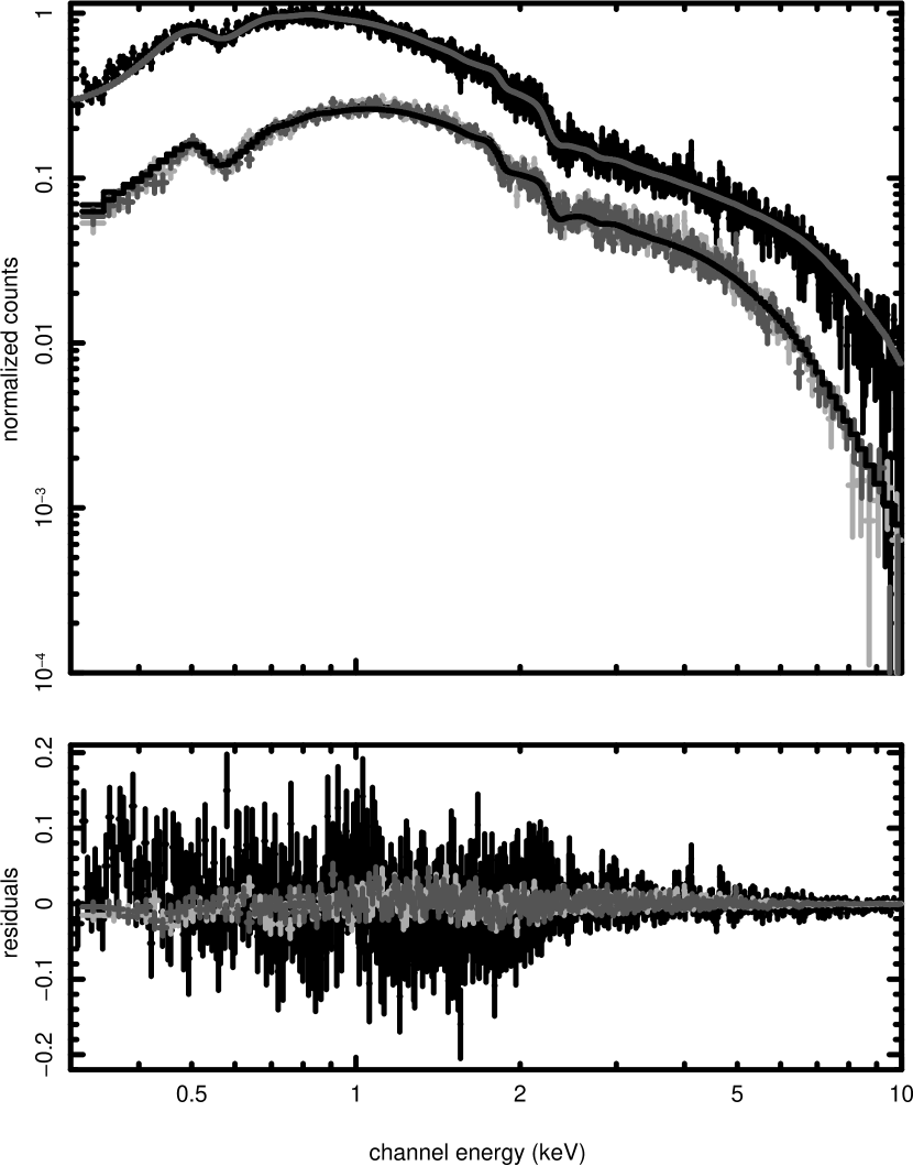
Figure 1.— EPIC spectrum of observation 0200980101 of Holmberg IX XMM1. This plot shows the spectrum fit with the tbvarabs*tbabs*edge*(grad + pow) model and the residuals from this fit. The best fit parameters are listed in Table 2.

The soft component of ULXs is most often modeled as a thermal component originating from an accretion disk surrounding a central black hole. There are numerous disk models applied to model this possibly thermal component. In Paper 1, we modeled this component as a simple blackbody (in XSPEC bbody). While an accretion disk is expected to have a range of temperatures, empirically a single blackbody is a good fit to low signal-to-noise spectra. A simple absorbed blackbody and power law model was used for Galactic black hole X-ray binaries in the 1980s when the quality of data for these sources was analogous to that for ULX sources today. As the next step in accretion disk models, the soft component of ULX spectra is often modeled as an optically thick, geometrically thin, multi-component blackbody disk (a multi-component disk or MCD model, diskbb in XSPEC) (Mitsuda et al., 1984).

Two disk models that are used to fit the soft component of ULX spectra with more physical accuracy are the XSPEC models diskpn and grad. The diskpn model is an extension of the MCD (diskbb) model which uses a pseudo-Newtonian potential. The grad model (Hanawa, 1989; Ebisawa, Mitsuda, & Hanawa, 1991) is a multi-component disk model that unlike the diskbb or diskpn model, incorporates the affects of general relativity. One of the advantages of the grad model is that it fits the spectra for mass (M_grad) and mass accretion rates ($\dot{M}$) given a few initial assumptions (distance to the source, disk inclination angle, and the ratio of the color temperature to the effective temperature).

In addition to thermal models, other models have been suggested to explain the soft component. Two of these models are ionized reflection and the warm absorber model. Both of these models have been applied to low-redshift PG Quasars, sources with blackbody temperatures of 150 eV. This is relevant to ULXs since many spectral fits of ULXs require cool accretion disk temperatures of approximately 100 eV (Miller et al., 2003; Miller, Fabian & Miller, 2004; Roberts et al., 2005; Winter, Mushotzky, & Reynolds, 2005). The reflection model suggests that the soft component results from X-ray ionized reflection. In this model, back-scattering and fluorescence of X-rays in the disk, as well as radiative recombination, cause elements with smaller ionization potentials (e.g. C, O, N) to become highly ionized. Ross & Fabian (2005) note that a relativistically blurred X-ray ionization model folded through an XMM-Newton pn response matrix, is well-fit by a blackbody with a temperature of 150 eV, the same value that is seen in PG Quasars and many ULXs. In the warm absorber model, absorption edges and lines from an absorbing material close to the X-ray source appear as a thermal component in poorer quality spectra. With increased spectral resolution, the numerous absorption edges and lines are distinguishable. The warm absorber may be the result of a strong, mildly relativistic wind from the disk as suggested by Gierliński & Done (2004). Indeed, the presence of a warm absorber is well known and studied in many Seyfert galaxies (e.g. NGC 3783 and MCG–6-30-15).

As noted above, for subsequent spectral fits we assume a thermal model for the soft component of the ULX spectra. In the following section (Section 4), we will discuss the effect different thermal models have on the measured absorption values. In order to measure the hydrogen column density, we fit the spectra of sources listed in Table 1 with the more sophisticated Tuebingen-Boulder ISM absorption model of Wilms, Allen, & McCray (2000) (tbabs, tbvarabs in XSPEC). This model accounts for X-ray absorption resulting from contributions from X-ray absorption from the gas phase of the ISM, grains, and molecules. The model uses updated solar abundances and photoionization cross-sections. For both the EPIC and RGS spectra, we accounted for Galactic hydrogen absorption by setting the column density of the tbabs model equal to the Milky Way hydrogen column density along the line of sight to the host galaxy . These column densities are quoted in Table 1 and are all less than $6\times 10^{20}$ cm^-2.

Since the measured X-ray column densities for ULXs are typically an order of magnitude higher than the Dickey & Lockman (1990) Milky Way values (Fig. 8 of Paper 1), we are confident that the additional absorption measured is not from the Milky Way. To determine the host galaxy’s hydrogen column density and the abundances of elements along the line of sight (oxygen and iron), we used the tbvarabs model. The tbvarabs model accounts for X-ray absorption due to photo-ionization. It includes the effects due to the H₂ molecule and depletion of metals in grains. The model allows for individual fits to abundant elements (He through Ni), H₂, and depletion of elements in grains. We initially allowed the hydrogen column density to vary, fixing all other tbvarabs parameters to their defaults. The Galactic column density remained fixed (using the tbabs model), while the other parameters (power law and blackbody components) were allowed to vary. This was modeled as tbabs*tbvarabs*(bbody + pow) in XSPEC, where tbabs was fixed to the Milky Way value and tbvarabs was used to fit the absorption from the ULX/host galaxy contribution. With the best-fit hydrogen column density (from tbvarabs), we allowed the oxygen abundance and then the iron abundance to vary from the solar abundances. Allowing these parameters to float provides measurements of the depth of the oxygen K-shell edge at 542 eV and the iron L-shell edge at 851 eV.

As in Baumgartner & Mushotzky (2006), we found that for our 14 sources, the oxygen absorption values from the tbvarabs model yielded different values for the EPIC pn and MOS spectra. Thus, we follow the procedure of Baumgartner & Mushotzky (2006) in adding an edge model to account for the differences. We add an extra edge component to the MOS1 and MOS2 detectors at an energy of 0.53 keV with optical depths of 0.22 and 0.20 respectively (modeled as tbabs*tbvarabs*edge*(bbody + pow)). This is the template model used for all spectral fits mentioned throughout the rest of the paper, where other thermal models are used in place of the simple blackbody (bbody) model as indicated.

An additional problem we note involves the hydrogen column densities along the line of sight. Baumgartner & Mushotzky (2006) note that a column density (n_H) greater than $0.5\times 10^{21}$ cm^-2 is necessary to allow for good oxygen abundance measurements. We also note that at very high n_H values the oxygen edge is undetectable, where high absorption values cause the signal-to-noise to be too low to detect the edge.

4. Nature of the Soft Component

In the previous section we outlined three possible origins for the soft component in ULXs (X-ray reflection, thermal emission from an accretion disk, and a warm absorber model). For our purposes, we assume a thermal component origin. We chose the thermal model since, as described in Paper I, the spectra of ULXs are well described with models used to fit Galactic black hole X-ray binaries. To gauge the effect different disk models (i.e. bbody, diskbb, diskpn, grad) may have on the measured abundances, we discuss different disk models in section 4.1. In section 4.3, we assess the usefulness of the model (absorbed disk and power law) for measuring the galactic/ULX hydrogen column density and the oxygen and iron abundances by discussing the physical plausibility of this model.

For sources with at least 5000 counts, the 14 sources listed in Table 1, we fitted the grad model for the soft-component of the spectra (XSPEC model tbabs*tbvarabs*edge*(grad + pow)). We assumed a disk inclination angle of 60 degrees and a ratio T${}_{color}/$T_eff = 1.7 (the default value, typical of stellar mass BH sources). In Table 2, we list the best-fit parameters for EPIC spectra using this model. Rows with no source name indicated represent an additional observation of the previous ULX (as indicated in Table 1). Table 3 provides the best-fit parameters for the RGS spectra. The important measurements to note are the host galaxy/ULX contribution to the hydrogen column density, oxygen abundance, and iron abundance from the tbvarabs model. All errors quoted in this paper are for the 90% confidence level for one degree of freedom ($\Delta\chi^{2}=2.76$). We provide a representative spectral fit in Figure 1 for the long observation of Holmberg IX XMM1.

4.1. Comparison of Thermal Disk Models

We chose the general relativistic disk model, grad, because it is the most physically accurate of the various simple accretion disk models. Also, the grad model requires few initial parameters while making a direct calculation of the mass and mass accretion rate of the black hole. In order to compare the grad results with an alternate model, we fit the highest signal-to-noise observation of Holmberg IX XMM1 with the diskpn model (with the inner radius of the disk set to the radius of marginal stability or 6 times the Schwarzschild radius) in place of the grad model. We found that the values obtained agreed with those of the grad model. The mass from the diskpn model was slightly lower at 358 M_☉ (corresponding to kT$=0.23$ keV) and the iron abundance was slightly higher at 2.33 compared to the grad model. Since the diskpn and grad models yield similar values, either of these disk models would be sufficient for determining the hydrogen column density and oxygen and iron abundances.

Table 4Alternate Thermal Model Spectral Fits to ULX Sources with $>20000$ Counts

Source	nH	Oxygen abundance	Iron abundance	kT	$\Gamma$	$\chi^{2}$/dof	counts
tbabs*tbvarabs*edge*(bbody + pow)
HolmII XMM1	0.12${}^{+0.01}_{-0.01}$	0.97${}^{+0.11}_{-0.12}$	0.0+0.32	0.24${}^{+0.01}_{-0.01}$	2.41${}^{+0.03}_{-0.03}$	2216.5/2018	342874
$\cdots$	0.14${}^{+0.03}_{-0.02}$	1.37${}^{+0.38}_{-0.39}$	4.38${}^{+0.62}_{-1.8}$	0.16${}^{+0.01}_{-0.01}$	2.31${}^{+0.08}_{-0.04}$	952.7/973	43116
HolmIX XMM1	0.14${}^{+0.02}_{-0.01}$	1.51${}^{+0.19}_{-0.15}$	3.37${}^{+0.99}_{-0.80}$	0.19${}^{+0.01}_{-0.01}$	1.40${}^{+0.02}_{-0.01}$	2856.7/2752	148061
$\cdots$	0.23${}^{+0.10}_{-0.04}$	1.37${}^{+0.43}_{-0.44}$	4.75${}^{+0.25}_{-1.94}$	0.17${}^{+0.02}_{-0.03}$	1.71${}^{+0.14}_{-0.06}$	559.5/880	28108
M33 X-8	0.22${}^{+0.01}_{-0.14}$	1.24${}^{+0.10}_{-0.10}$	2.38${}^{+0.31}_{-0.60}$	0.76${}^{+0.02}_{-0.02}$	2.51${}^{+0.07}_{-0.06}$	1528.8/1533	123903
M81 XMM1	0.39${}^{+0.03}_{-0.02}$	1.13${}^{+0.15}_{-0.07}$	1.78${}^{+0.65}_{-0.40}$	0.90${}^{+0.03}_{-0.02}$	2.70${}^{+0.05}_{-0.05}$	1240.2/1241	69776
$\cdots$	0.26${}^{+0.09}_{-0.04}$	1.46${}^{+0.26}_{-0.49}$	1.61${}^{+2.02}_{-1.61}$	0.99${}^{+0.38}_{-0.28}$	1.76${}^{+0.13}_{-0.09}$	627.4/668	31731
NGC253 XMM2	0.22${}^{+0.05}_{-0.05}$	1.21${}^{+0.40}_{-0.37}$	1.53${}^{+1.67}_{-1.53}$	0.73${}^{+0.14}_{-0.11}$	2.16${}^{+0.08}_{-0.23}$	460.8/496	20651
tbabs*tbvarabs*edge*(diskbb + pow)
HolmII XMM1	0.11${}^{+0.001}_{-0.01}$	0.65${}^{+0.09}_{-0.05}$	0.0+0.06	0.34${}^{+0.02}_{-0.02}$	2.38${}^{+0.05}_{-0.04}$	2241.8/2018	342874
$\cdots$	0.15${}^{+0.03}_{-0.02}$	1.05${}^{+0.34}_{-0.38}$	2.67${}^{+1.65}_{-1.71}$	0.21${}^{+0.04}_{-0.01}$	2.27${}^{+0.06}_{-0.07}$	954.2/973	43116
HolmIX XMM1	0.19${}^{+0.02}_{-0.02}$	1.38${}^{+0.11}_{-0.16}$	2.39${}^{+0.58}_{-0.84}$	0.24${}^{+0.02}_{-0.01}$	1.39${}^{+0.02}_{-0.03}$	2878.9/2752	148061
$\cdots$	0.30${}^{+0.11}_{-0.07}$	1.36${}^{+0.32}_{-0.38}$	4.03${}^{+0.97}_{-1.65}$	0.20${}^{+0.04}_{-0.03}$	1.72${}^{+0.10}_{-0.07}$	559.8/880	28108
M33 X-8	0.19${}^{+0.04}_{-0.03}$	1.04${}^{+0.15}_{-0.16}$	1.75${}^{+0.68}_{-0.71}$	1.17${}^{+0.05}_{-0.05}$	2.47${}^{+0.21}_{-0.15}$	1530.4/1533	123903
M81 XMM1	0.63${}^{+0.08}_{-0.15}$	1.19${}^{+0.09}_{-0.15}$	2.07${}^{+0.40}_{-0.69}$	1.38${}^{+0.03}_{-0.08}$	4.08${}^{+0.75}_{-0.59}$	1247.7/1241	69776
$\cdots$	0.27${}^{+0.18}_{-0.08}$	1.42${}^{+0.57}_{-0.49}$	1.63${}^{+1.69}_{-1.63}$	2.06${}^{+0.55}_{-0.97}$	1.98${}^{+1.40}_{-0.58}$	626.9/668	31731
NGC253 XMM2	0.21${}^{+0.10}_{-0.07}$	1.16${}^{+0.53}_{-0.37}$	1.64${}^{+1.64}_{-1.64}$	1.27${}^{+0.22}_{-0.27}$	2.27${}^{+0.83}_{-0.62}$	461.3/496	20651

In order to test the effect the thermal model has on the tbvarabs measured parameters (i.e. n_H and abundances), we wanted to compare the results from the more physical disk model (grad) with less physical models (bbody and diskbb). In order to compare the results from these three models, we chose to examine the best-fit parameters for spectra with the highest signal-to-noise (using sources with at least 20000 counts). Thus, in Table 4 we list the best-fit parameters obtained using an absorbed blackbody and power law (tbabs*tbvarabs*edge*(bbody + pow)) and an absorbed diskbb and power law model (tbabs*tbvarabs*edge*(diskbb + pow)) for sources with at least 20000 counts. Subsequently in this paper, when we refer to the bbody, diskbb, or grad models, we are referring to the model fits used in Tables 2- 4.

The curvature, or shape of the spectra at low energies, for the bbody, diskbb, and grad models is different, presumably affecting the column density and absorption values. From a comparison of these models, comparing the mean values from all of the observations with $>20000$ counts listed in Tables 2 and 4, we find that the column densities obtained with the diskbb model are nearly identical to those with the grad model (the exception is the source NGC 253 XMM2). The MCD (diskbb) model hydrogen column densities are approximately 6% higher than those of the blackbody model (excluding the first M81 XMM1 observation). The average power law indices for the three models agree within a factor of 5%, with the bbody model having the lowest and the grad having the highest average power law index (excluding the first M81 XMM1 observation). Thus, the difference in both power law index and hydrogen column density is negligible on average, with the exceptions of NGC 253 XMM2 and M81 XMM1.

For a comparison of the derived abundances, the oxygen abundance is roughly the same between the grad and bbody model. These values are approximately 10% higher than those derived from the MCD (diskbb) model. The iron abundances, however, vary more from model to model. The blackbody model average iron abundance is $\approx 13$% higher than that of the grad model and $\approx 18$% higher than that of the diskbb model. Thus, there are no significant changes to the model parameters in changing the base accretion disk model. These results are verified by simulations described in the appendix.

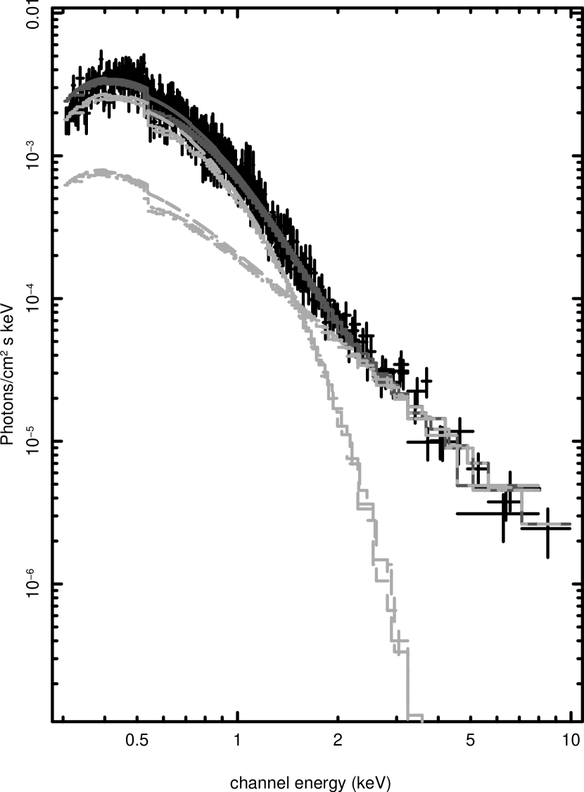
Figure 2.— Plot of the EPIC unfolded spectrum for the NGC 5408 XMM1 ULX with the high mass solution (see Table 2). With the spectrum, the absorbed grad and absorbed power law model components are plotted with light gray lines while the combined model is plotted in dark gray. The thermal component clearly dominates the low energy spectrum with this model.

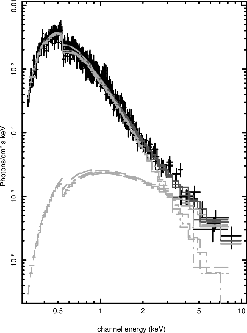
Figure 3.— Plot of the EPIC unfolded spectrum for the NGC 5408 XMM1 ULX with the low mass solution (see Table 5). With the spectrum, the absorbed grad and absorbed power law model components are plotted with light gray lines while the combined model is plotted in dark gray. Notice that the low energy spectrum is dominated by the power law component with a weak contribution from the disk model (grad).

4.2. Degenerate Model

In modeling our sources with the tbvarabs*tbabs*edge*(grad+pow) model, we found that some of the ULX sources were well-fit by a model where the power law component dominates the low energy spectrum, also seen in Stobbart, Roberts, & Wilms (2006). This type of spectral fit typically yields a steeper power law index ($\Gamma>3.0$) and a low mass (M$<10$ M_☉). For two sources, M33 X-8 and M81 XMM1, this model fit was a much better fit than a higher mass model with $\Delta\chi^{2}$ of 476 and 190 respectively. However, for some sources, there was a degeneracy between the two models (high mass and low mass/steep power law). We illustrate this degeneracy with observation 0112290601 of the source NGC 5408 XMM1, showing the high mass model and spectral fit in Figure 2 and the low mass model and spectral fit in Figure 3. For spectra exhibiting this degenerate solution, we include the low-mass/steep power law fits in Table 5. These fits all exhibit, in addition to low masses, solutions with $\dot{M}>>\dot{M}_{Edd}$.

Table 5Spectral Fits for EPIC spectra with tbabs*tbvarabs*edge*(grad + pow) model for Sources with Degenerate Solution (Low Mass/Steep Power Law)

Source	nH	O abund.	Fe abund.	Mass (M☉)	$\dot{M}/\dot{M}_{Edd}$	$\Gamma$	$\chi^{2}$/dof	counts
HolmII XMM1	0.20${}^{+0.04}_{-0.04}$	0.83${}^{+0.17}_{-0.27}$	1.11${}^{+0.83}_{-1.11}$	2.24${}^{+1.52}_{-1.24}$	7.79${}^{+1.52}_{-1.95}$	3.10${}^{+0.31}_{-0.30}$	0.99	43116
HolmIX XMM1	0.39${}^{+0.13}_{-0.12}$	1.05${}^{+0.21}_{-0.33}$	2.08${}^{+0.95}_{-1.45}$	3.91${}^{+1.47}_{-1.59}$	22.0${}^{+1.79}_{-2.86}$	3.51${}^{+0.79}_{-0.87}$	0.64	28108
NGC253 XMM2	0.18${}^{+0.17}_{-0.08}$	1.10${}^{+0.42}_{-0.55}$	1.32${}^{+1.90}_{-1.32}$	6.82${}^{+4.19}_{-2.22}$	1.27${}^{+0.71}_{-0.40}$	2.15${}^{+0.84}_{-0.58}$	0.93	20651
NGC5204 XMM1	0.18${}^{+0.05}_{-0.04}$	1.00${}^{+0.30}_{-0.40}$	0.0${}^{+0.59}_{-0.0}$	3.21${}^{+0.98}_{-0.95}$	6.86${}^{+0.67}_{-0.09}$	3.28${}^{+0.39}_{-0.38}$	0.95	16717
$\cdots$	0.20${}^{+0.06}_{-0.05}$	0.63${}^{+0.35}_{-0.48}$	0.0${}^{+0.62}_{-0.0}$	2.95${}^{+2.13}_{-1.84}$	7.37${}^{+1.35}_{-2.08}$	3.16${}^{+0.50}_{-0.44}$	0.94	13864
NGC300 XMM1	0.21${}^{+0.05}_{-0.03}$	1.59${}^{+0.22}_{-0.26}$	0.0${}^{+0.53}_{-0.0}$	1.69${}^{+0.85}_{-0.32}$	0.73${}^{+0.18}_{-0.13}$	3.89${}^{+0.21}_{-0.32}$	1.00	11479
N4559 X-7	0.20${}^{+0.06}_{-0.05}$	0.34${}^{+0.38}_{-0.34}$	0.0${}^{+0.48}_{-0.0}$	5.79${}^{+2.82}_{-2.75}$	6.63${}^{+1.44}_{-2.42}$	3.13${}^{+0.55}_{-0.50}$	0.83	12506
NGC5408 X-1	0.18${}^{+0.05}_{-0.04}$	0.87${}^{+0.28}_{-0.42}$	0.45${}^{+1.75}_{-0.45}$	2.29${}^{+1.57}_{-1.28}$	4.87${}^{+1.23}_{-1.02}$	4.09${}^{+0.28}_{-0.34}$	0.89	10045

In Stobbart, Roberts, & Wilms (2006), the authors discussed the same issues in fitting the XMM spectra of 13 ULXs. They found that two sources, M33 X-8 and NGC 2403 X-1, were best fit by the model with a power law fit to the low energy portion and thermal model at higher energy. They also indicated six sources where an ambiguity existed between the two models. To understand the spectra of the sources where both models provided good fits to the data, we further investigated the spectra of sources with multiple observations.

For Holmberg II X-1 and Holmberg IX X-1 our spectral fits include multiple observations (a shorter and a 100 kilo second observation). For each of these sources, we found that the shorter observation could be fit with either a high mass or low mass solution. When we fit the 100 kilo second observation, however, the high mass model was a much better fit. The $\Delta\chi^{2}$ values between the high mass and low mass solutions for the kilo second observations were 135 and 88, respectively. To test this further, we also fit a 100 kilo second observation of NGC 5408 XMM1 with both of these models. This observation (0302900101) is a proprietary observation whose spectral and temporal analysis will appear in Strohmayer et al. (in prep). We processed the pn data with SAS 6.5, following the same procedure as noted in the Data Reduction section. Fitting the spectrum with both models (high mass and low mass solution) we found a $\Delta\chi^{2}$ value of 170, favoring the high mass model.

Thus, we find that for sources that are well fit by either model (showing a degenerate solution of either high mass or low mass/steep power law) the high mass solution is the best fit when a higher count spectrum is obtained (as for Holmberg IX XMM1, Holmberg II XMM1, and NGC 5408 X-1). Though we list the alternate model column density and absorption values in Table 5, we use the parameters listed in Table 2 throughout the paper (the high mass solutions).

As noted, M33 X-8 and M81 XMM1, sources with very high number of counts, were not well-fit with a standard disk at low energy, power law at high energy model. They were best fit with the steep low energy power law and hot disk model shown in Figure 3. Along with these sources, NGC 4559 X-10 and M83 XMM1 were also well-fit by this model. We will further discuss these sources in the following subsection.

Figure 4.— Black hole mass versus mass accretion rate (per Eddington accretion rate) obtained from the general relativistic disk model (grad). The sources with model parameters indicating high masses correspond to accretion rates that are below 40% of the Eddington accretion rate for the given mass. In Paper 1, we noted a temperature gap in the range of 0.26 keV to 0.50 keV from spectral fits utilizing an absorbed blackbody and power law model. In this figure, we see that there is a gap in mass from the parameters of the absorbed general relativistic disk and power law model. The values shown are results for the EPIC spectra only, as recorded in Table 2 (for all sources in Table 2). Therefore, there are multiple points for the sources with multiple observations. We plotted these sources (Holmberg II XMM1, Holmberg IX XMM1, M81 XMM1, and NGC 5204 XMM1) twice to confirm that their masses, as determined by the grad model, do not vary.

4.3. Physical Plausibility of the Accretion Disk models

In Paper 1, we had found that ULX spectra are consistent with the high/soft and low/hard states of Galactic black holes. We had classified the sources in this study as consistent with the high/soft state. The high/soft state, as stated earlier, is characterized by emission from an accretion disk and a Comptonized power law tail. In order to investigate whether the mass and accretion rate results from the grad model make physical sense in terms of the X-ray binary model, we present a comparison of the derived accretion rate in Eddington accretion rate versus the mass in Figure 4. The parameter $\dot{M}_{Edd}$ was computed as $\dot{M}_{Edd}=\frac{1.3\times 10^{38}M}{\eta c^{2}}$ where $\eta$, the efficiency factor, was set to 0.06 and M is the value M_grad. We find that for the sources with M${}_{grad}>100$ M_☉, the accretion rate is computed to be below 40% of the Eddington rate. This is assuming, as the grad model assumes, a Schwarzschild black hole. Noting that $\dot{M}/\dot{M}_{Edd}$ is equivalent to L $/$ L_Edd for most disk solutions, the L $/$ L_Edd values for the sources with M${}_{grad}>100$ M_☉ are consistent with those of Galactic black hole X-ray binaries in the high state (L $/$ L${}_{Edd}\approx 0.05-1.0$) (McClintock, Narayan, & Rybicki, 2004). Thus, the sources with M${}_{grad}>100$ M_☉ do have accretion rates that are predicted from scaling up (in mass) observed high state Galactic black holes. In addition, the spectral fit parameters for NGC 4631 XMM1, with an estimated mass of 5.5 M_☉ and an accretion rate L $/$ L_Edd of 0.84, are also consistent with the standard high state Galactic black hole model. This source is likely a normal stellar mass black hole X-ray binary in an external galaxy.

The remaining sources with M${}_{grad}<<100$ M_☉ (M33 X-8, M81 XMM1, NGC 4559 X-10, and M83 XMM1) yielded L $/$ L_Edd ratios in the range of 1 - 3. These sources are also those described in the previous section where the power law component fits the low energy spectrum. They are also well fit by a Comptonization model and correspond to a sub-class of high luminosity ULXs described in Paper 1. Due to the luminosity and modeled disk temperature (kT $\approx 1$ keV), we suggested that these sources were very high state stellar mass black hole systems. In order to be consistent with the black hole accretion model assumed in this study, the spectra of these sources should be the result of Comptonization from a thermal disk spectrum.

To test this further, we fit the spectrum of the highest count source of this type (M33 X-8) with an absorbed thermal disk and Comptonization model (tbabs*tbabs*(diskpn + comptt)). The comptt model has the parameters: a seed temperature (keV), a plasma temperature (keV), and optical depth of the medium. We used the diskpn model in place of the grad model since the former provides a disk temperature to which the comptt seed temperature can be fixed. This provides a physical model, where the thermal disk supplies the energy for the Compton tail. M33 X-8 was well fit by this model with a $\Delta\chi^{2}$/dof = 1659.9/1534 (1.08). Thus, these sources are still consistent with the black hole accretion model. Replacing the tbabs model used for the galactic column density with the tbvarabs, we measured the column density, oxygen abundance, and iron abundance. With this thermal disk and Comptonization model we obtained n${}_{H}=1.5^{+0.04}_{-0.08}\times 10^{21}$ cm^-2, O/H $=1.26^{+0.08}_{-0.15}$, and Fe/H $=2.83^{+0.71}_{-0.76}$, with a $\Delta\chi^{2}$/dof = 1577.3/1534 (1.03). Within the error bars, these results are consistent with those seen in Table 2.

5. Properties of the ISM in ULX Host Galaxies

The major question to be examined in using ULXs as probes of the ISM is whether the hydrogen column density and element abundances are primarily from the host galaxy or intrinsic to the local environment of the ULX. Before we can answer this question, it is important to understand the intrinsic spectrum of the source. In the previous section we discussed the nature of the soft component in light of the high signal-to-noise spectra of the 14 ULX sources we examined. We found that if the spectrum is due to thermal emission from a disk, modeling the spectrum with a variety of disk models (grad, diskbb, diskpn, bbody) does not significantly change the measured oxygen abundance or hydrogen column density.

Assuming the reliability of the hydrogen column density and abundance measurements, based on their model independent values, we investigate the source of the absorption in ULX spectra. In order to determine whether the model n_H values suggest the necessity of extra local absorption, we compare the model values with column densities obtained from H I studies. We investigate this in section 5.1. The oxygen abundances (as an indication of metallicity), which we examine in section 5.2, can provide further clues of whether the absorption we see in the X-ray spectrum is intrinsic to the source. We also examine possible connections between the host galaxy’s star formation rate and elemental abundances.

Figure 5.— Hydrogen column density from E_B-V (triangle) or H I studies (circle) vs. the hydrogen column density obtained from the tbvarabs model. H I column densities were obtained for Holmberg II, NGC 5204, and NGC 4559 through the WHISP survey (Swaters et al. 2002). Additional H I column densities were obtained for NGC 247, Holmberg IX, and M81 through VLA data (Braun 1995). The X-ray spectral fit columns are not biased towards significantly higher values than the alternate method column densities. This implies that most of the matter in the line of sight is from H I. This is not true, however, for the source M81 XMM1 (represented by the two outlying points in the lower left portion of the graph) where the X-ray column density is much greater than those from the optical and radio.

5.1. Column Densities

To determine whether the ULX X-ray hydrogen column densities represent largely galactic column densities or column densities local to the ULX, we compared the X-ray values to those obtained from optical and radio studies. For a comparison to hydrogen column densities from optical studies, we used interstellar reddening values. In a study of dust scattering X-ray halos surrounding point sources and supernova remnants, Predehl & Schmitt (1995) derived a relationship between hydrogen column density and interstellar reddening, using X-ray data. They found that n${}_{H}=5.3\times 10^{21}cm^{-2}E_{B-V}$. They also found that these X-ray derived column densities are not affected by the intrinsic absorption of the X-ray source. Thus, the optical reddening, $E_{B-V}$, becomes a useful tool in checking our own X-ray derived column densities. Through a literature search, we found E_B-V values for the sources M33 X-8 (0.22; Long, Charles, & Dubus (2002)) and M81 XMM1 (0.23; Kong et al. (2000)). The corresponding $E_{B-V}$-derived n_H values are plotted in Figure 5 as triangles.

Table 6Column Densities from Optical and H I Studies

Source	nH	Method
NGC 247 XMM1	0.316	H I
M33 X-8	0.170	EB-V
HolmII XMM1	0.157	H I
M81 XMM1	0.122	EB-V
M81 XMM1	0.078	H I
HolmIX XMM1	0.148	H I
NGC 4559 X7	0.357	H I
NGC 4559 X10	0.300	H I
NGC 5204 XMM1	0.182	H I

For a comparison of X-ray derived hydrogen column densities with radio values, we obtained H I column densities for four objects (Holmberg II XMM1, NGC 4559 X7, NGC 4559 X10, and NGC 5204 XMM1) from the WHISP catalog (Swaters et al., 2002). These are radio H I column densities within the host galaxy (galactic), not the Galactic/Milky Way columns. Exact values of the H I column densities were computed and given to us by Rob Swaters. Additionally, we include H I column densities of NGC 247 XMM1, M81 XMM1, and Holmberg IX XMM1 from Braun (1995). We obtained the FITS files of H I column density maps from this paper (available on NED), where the pixel value corresponds to the galactic column density in units of $10^{18}$ cm^-2. The H I n_H values from both studies are plotted in Figure 5 as circles. The column densities, from the radio and reddening studies, are listed in Table 6.

We find that the host galaxy column densities from alternate methods (optical or radio studies) are not significantly different from the X-ray column densities. Particularly, the X-ray values are not skewed towards substantially higher values than the optical/radio values. Thus, the X-ray columns are likely the galactic values without any additional local absorption. The exception, however, is M81 XMM1 (represented by 2 points in Figure 5, one for each of the methods). The E_B-V value ($1.22\times 10^{21}$ cm^-2) and the H I value ($0.78\times 10^{21}$ cm^-2) are significantly lower than the X-ray column density. This may indicate the presence of extra absorption around this source.

The result that the X-ray hydrogen column densities are in good agreement with those from H I studies and interstellar extinction values is interesting considering that the X-ray measured column densities are along a direct line of sight to the ULXs while the H I measurements are an average over a larger beam area. The agreement between the two measurements implies that the ULX sources, with the exception of M81 XMM1, lie within roughly normal areas of their host galaxies (i.e. not in regions of higher column density such as a molecular cloud).

5.2. Elemental Abundances

5.2.1 Test for Oxygen Ionization Level

Before discussing implications of the determined oxygen and iron abundances, we relate a test performed to determine whether we could distinguish between different ionization levels of oxygen. To do this, we used the absorption edge model, edge, in XSPEC (using the full model: tbabs*tbvarabs*edge*edge*(grad + pow)). We first checked to see that the abundance values obtained with the edge model matched the values from the tbvarabs model. We fixed the oxygen abundance in the tbvarabs model at zero and added the edge model, allowing the threshold energy and absorption depth ($\tau$) to float as free parameters (with an initial energy set to 0.543 keV). We fit this model to the longest observations of Holmberg II XMM1 and Holmberg IX XMM1 in addition to a source with a lower number of counts, NGC 5408 XMM1 (0112290601).

To find the oxygen column density (n_O), we used the relationship that $\tau=\sigma\times n_{O}$, where $\sigma$ is the cross section for photoabsorption. We used the cross section values for neutral oxygen published in Reilman & Manson (1979) as an estimate. This choice is supported by the results of Juett, Schulz, & Chakrabarty (2004), who measured the ratio of oxygen ionization states in the ISM as O II/O I$\approx 0.1$. In Table 7, the hydrogen column density, threshold energy, and optical depth are listed for the sources fit with this model. From Reilman & Manson (1979) we used the cross section values of $\sigma=5.158\times 10^{-19}$ cm² (for $E=0.540$ keV) and $\sigma=4.789\times 10^{-19}$ cm² (for $E=0.570$ keV). As seen in Table 7, the hydrogen column densities and the oxygen abundances obtained from this model are close to those from the tbvarabs model. The [O/H] values, where [O/H] = 12 + log(O/H) and O and H represent oxygen column density and hydrogen column density respectively, between the two models vary by less than 1%.

To test whether the threshold energy from the edge model is affected by the ionization level of oxygen, we simulated spectra of an absorbed power law model with an oxygen edge. Tim Kallmann (P.C.) provided us with an oxygen edge model incorporating the cross sections of Garcia et al. (2005). The model allows for a variation of the ratio of O II/O I. Using the response and ancillary response matrices from the long Holmberg II ULX observation, we simulated spectra with the XSPEC fakeit command for a $\Gamma=2.35$ power law. We simulated spectra for O II/O I ratios of 0.0, 0.2, 0.4, 0.6, 0.8, and 1.0. The simulated spectra were binned with a minimum of 20 counts/bin. The absorption edge component of the spectrum was then fit with the edge model. The fits to the threshold energies for the simulated spectra yielded values ranging from 0.53-0.59 keV, with no preference of lower O II/O I ratios corresponding to lower threshold energies. Since the O I absorption edge occurs at E$=0.543$ keV and the O II absorption edge occurs at E$=0.57$ keV, we could not distinguish between these ionization states of oxygen. Our simulations show that the oxygen edge measurements will be sensitive to O I and O II but not to high ionization states (for instance O VIII which has an edge energy of 0.87 keV).

Figure 6.— Oxygen abundances from studies of H II regions vs. oxygen abundances from the tbvarabs model. The [O/H] ratios are given for Holmberg II XMM1, NGC 5408 XMM1, Holmberg IX XMM1, NGC 4559 XMM1, NGC 4559 XMM2, NGC 1313 XMM3, M33 X-8, NGC 300 XMM1, NGC 253 XMM2, and M81 XMM1 using the P-calibration method (circle). Also, [O/H] ratios are included for M33 X-8, NGC 300 XMM1, M81 XMM1, NGC 253 XMM2, and M83 XMM1 using the R₂₃ calibration method (triangle). Arrows indicate that the lower limit for the [O/H] X-ray parameter is below the plotted graph region. Our values are high compared to the P-method but in good agreement with the R₂₃ method. The sources with the largest difference between [O/H] values are those located in irregular galaxies.

5.2.2 X-ray/optical [O/H] Comparison

As noted above, we tested the oxygen abundances obtained with the absorption model tbvarabs against the abundances obtained from adding a photo-electric absorption edge model, for three of the ULX sources. We found good agreement ($<1$% difference in [O/H] values) between both models for the X-ray spectra. However, we found that it is not possible to distinguish between different low ionization states of oxygen using the edge model.

Table 7Spectral Fits for Oxygen Edge with tbabs*tbvarabs*edge*edge*(grad + pow) model

Source	nH	E	$\tau$	nO	[O/H]	$\chi^{2}$/dof	counts
HolmII XMM1	0.16${}^{+0.01}_{-0.01}$	0.566${}^{+0.01}_{-0.01}$	0.35${}^{+0.02}_{-0.01}$	7.2	8.65/8.64	2543/2017	342874
HolmIX XMM1	0.19${}^{+0.02}_{-0.02}$	0.543${}^{+0.01}_{-0.01}$	0.62${}^{+0.11}_{-0.12}$	12.0	8.81/8.82	2887/2751	148061
NGC 5408 XMM1	0.17${}^{+0.06}_{-0.03}$	0.538${}^{+0.04}_{-0.02}$	0.37${}^{+0.29}_{-0.21}$	7.1	8.61/8.63	298/334	10045

We now discuss comparisons of our X-ray oxygen absorption values with measurements in different wavelengths, based on a literature search for [O/H] ratios. In Figure 6 we compare our [O/H] ratios with those of a study conducted by Pilyugin, V$\acute{i}$lchez, & Contini (2004) (circles). They provide a compilation of [O/H] ratios determined through spectrophotometric studies of H II regions. Their [O/H] values are based on the radial distribution of oxygen abundance using the P-method. They determined [O/H] values for spiral galaxies where published spectra were available for at least 4 H II regions. In addition, they reference [O/H] values for irregulars obtained through alternate methods. Our [O/H] values are determined from the oxygen abundances listed in Table 2. Thus, [O/H]$=12+\log(O\times 0.00049)$. O is the oxygen abundance obtained from the model, which is multiplied by the Wilms relative abundance of $4.9\times 10^{-4}$ of oxygen to hydrogen. We were able to compare [O/H] values for the sources located in M33, NGC 253, NGC 300, M81, Holmberg II, NGC 4559, and NGC 5408. We include the [O/H] value computed for the Holmberg IX ULX by Miller (1995) of 8.12. This value was computed from an optical study of the surrounding H II region. Also, we add the [O/H] value of 8.4 for NGC 1313, determined separately by both Calzetti & Kinney (1994) and Walsh & Roy (1997).

As shown in Figure 6, our [O/H] values are consistently high compared to those obtained from the Pilyugin, V$\acute{i}$lchez, & Contini (2004) H II study. Pilyugin, V$\acute{i}$lchez, & Contini (2004) include a discussion of how their values, obtained by the P-calibration method, are significantly lower than those obtained by Garnett (2002) using the R₂₃-calibration method. In Figure 6 we include [O/H] values for NGC 253, NGC 300, M33, M81, and M83 from Garnett (2002) (triangles). Our oxygen abundances are in much better agreement with the values from this R₂₃-calibration method.

Our [O/H] values, which are consistent in the X-ray band between two separate absorption models, (tbabs*tbvarabs*edge*(grad + pow) and an tbabs*edge*edge*(grad + pow) model), are consistent with the values of Garnett (2002). We further wish to compare them to the metallicity predicted from Sloan Digital Sky Survey (SDSS) results. As a result of a SDSS study, Tremonti et al. (2004) found a luminosity-metallicity relation for their sample of star-forming galaxies of: $12+\log(O/H)=-0.185(\pm 0.001)M_{B}+5.238(\pm 0.018)$. In Figure 7 we compare our values with their results (represented by the line). We obtained absolute magnitudes (M_B) for the host galaxies using the total apparent corrected B-magnitude recorded in the HyperLeda galaxy catalogue (Paturel et al., 1989)(parameter btc) and the distances listed in Table 1 of Paper 1. For M33 and NGC 4559, which were not included in the previous study, we used the distances of 0.7 Mpc and 9.7 Mpc from Ho et al. (1997). The majority of our sources are consistent with the SDSS results. However, the sources in irregular galaxies have metallicities much higher than predicted.

5.2.3 Galaxy Properties

More luminous galaxies are sometimes expected to have higher star formation rates, and thus higher metallicity. However, we found no evidence of this. Investigating further into the relationship between star formation rate (SFR) and metallicity, we chose to look at a galactic luminosity diagnostic that is less dependent on extinction from dust, the infrared galactic luminosity (L_FIR). In Paper 1, we calculated L_FIR using data from the Infrared Astronomical Satellite and the approach of Swartz et al. (2004). We quoted values of L_FIR in Paper 1. Using the same method, with IRAS fluxes obtained from Ho et al. (1997), we find M33 to have L${}_{FIR}\approx 1.7\times 10^{42}$ erg s^-1 and NGC 4559 to have L${}_{FIR}\approx 7.4\times 10^{42}$ erg s^-1. We used these L_FIR values to compare the SFR to both the oxygen and iron abundances.

Figure 7.— Host galaxy M_B vs. ULX X-ray [O/H] ratio. The solid line represents the SDSS results from a study of star-forming galaxies (Tremonti et al., 2004). Arrows indicate that the lower limit for the [O/H] X-ray parameter is below the plotted graph region. Our values are largely consistent with the Sloan results, with the exception of Holmberg IX and Holmberg II. Both of these galaxies are irregulars. The X-ray [O/H] ratio derived from the ULX spectra is higher than predicted for these objects.

Figure 8.— Oxygen abundance ([O/H]) as a function of the host galaxy’s FIR luminosity, obtained from IRAS. The line represents the Wilms solar value of [O/H] . Arrows indicate that the lower limit for the [O/H] X-ray parameter is below the plotted graph region. There appears to be no correlation between L_FIR and oxygen abundance. In fact, the sources show roughly solar [O/H] abundances regardless of host galaxy.

Figure 9.— Iron abundance ([Fe/H]) as a function of the host galaxy’s FIR luminosity obtained from IRAS. Holm IX did not have corresponding IR data, however, being an irregular galaxy, its L_FIR would probably be comparable to Holm II. The iron abundances of both of the irregulars are well above those of the ULXs in spiral galaxies. The sources in galaxies with larger L_FIR have roughly equal iron abundances, within the error bars. The iron abundances in all cases are well above the Wilms solar abundance. Arrows indicate that the lower limit for the [Fe/H] X-ray parameter is below the plotted graph region.

Figure 10.— [Fe/H] as a function of [O/H] from the tbvarabs model, using the grad and power law fit. The Wilms solar abundance is indicated with an open circle. The ratio of Fe/O abundances obtained through the X-ray spectral fits are approximately the Wilms solar values. Arrows indicate that the lower limit for the [Fe/H] X-ray parameter is below the plotted graph region.

Figure 11.— Oxygen abundances from the tbvarabs model vs. distance of the ULX from the host galaxy’s dynamical center. The [O/H] ratios are given for spiral galaxies only. There is no correlation between radius and oxygen abundance in our sample. However, since the sources originate in different host galaxies with different abundances, there is no conclusion that can be drawn from this data. The host galaxy NGC 4559, containing two ULX sources studied, does appear to show a possible correlation (the source nearer the center has a higher oxygen abundance), however, the error bars on the oxygen abundance are large for both sources.

In Figure 8, we plot oxygen abundance relative to SFR. All sources with the exception of Holmberg IX XMM1, which did not have available IRAS data, are plotted. We see, as was also illustrated in Figure 7, that the luminosity of the host galaxy does not determine the metallicity. The more luminous galaxies do not have metallicities higher than the less luminous galaxies. In fact, most sources have oxygen abundances that are roughly the Wilms solar abundances (indicated by the line).

In Figure 9 we see that there is no relationship between iron abundance (see values in Tables 2 and  3 for values) and SFR. The Wilms solar abundance for iron is only $2.69\times 10^{-5}$ relative the hydrogen abundance. The plots show that the metallicity relationship is very flat, all of the sources have roughly solar abundances. This is also seen in Figure  10. This plot shows the [Fe/H] ratios versus the [O/H] values, both obtained through the tbvarabs model. The solar Wilms values are represented on the plot by the open circle symbol. It appears that the sources are slightly more abundant in iron than the solar value, however, the error bars are quite large. The oxygen abundances, as before stated, are roughly the solar Wilms value. Roughly, the abundances appear solar.

With such a flat relationship between abundance and luminosity, we tested to see if this result carried through in a comparison of abundance versus radial distance within the host galaxy. This follows upon an interesting property observed in spiral galaxies. Namely, that abundances are typically higher in the center of the galaxy and decrease with increasing radius (Searle, 1971). We tested how our results compare to this result in Figure  11. For the sources located within spiral galaxies, we plotted the [O/H] ratio as a function of distance R from the dynamical center (as reported by NED). We used the distances quoted in Table 1 of Paper 1 to translate angular distance on the sky into kpc from the galactic center. As evidenced in the plot, we do not see much variation in the [O/H] values. Clearly, the expected scaling of higher oxygen abundance towards the center is not seen. Since the sources lie in different host galaxies with different relative abundances, it is possible that this trend may be detectable with a larger sample of galaxies. However, the implication from Figures 7 through 11 is that the environment of the ULX sources is relatively uniform in terms of metallicity. The ULX sources appear to live in similar environments, with metallicities roughly solar.

6. Summary

Through our work, we conclude that X-ray spectral fits to ULX sources do provide a viable method of finding abundances in other galaxies. We have determined hydrogen column densities and oxygen abundances along the line of sight to 14 ULX sources. To measure these values, we assumed a connection between ULXs and Galactic black hole systems such that the ULX spectra used in this study correspond to a high/soft state. Therefore, we modeled the sources with an absorbed disk model and power law (in XSPEC tbabs *tbvarabs*(accretion disk model + pow)). We tested the effect different accretion disk models have on the measurement of the host galaxy’s hydrogen column density and elemental abundance with the disk models: grad, diskpn, diskbb, and bbody. We found that the measured hydrogen column density and abundances are model independent.

We also tested the physical plausibility of this model by comparing the mass and mass accretion rates obtained from the grad model with expected results based on Galactic black hole systems. We found that the ULX spectra were consistent with the high/soft state, with $L/L_{Edd}$ values $<1.0$ for sources with a standard thermal model at low energies and power law dominated higher energy spectrum. For four sources, the spectra were consistent with a heavily Comptonized spectrum. These sources are more likely stellar mass black hole systems in a very high state of accretion. We modeled their spectra with a power law at low energy and disk model around 1 keV. This model provided similar column density and abundance values to a more physical absorbed disk and Comptonization model.

Comparing our X-ray measured column densities with those from optical and H I studies for 8 of our sources, we find that 7 of the sources have X-ray column densities approximately equal to those of the alternate methods. This implies that the hydrogen columns towards most of our ULX sources represent that of their host galaxy. Since the H I studies represent averages over a large beam area where the X-ray column densities are directly along the line of sight to the ULX source, this implies that the ULX sources lie within roughly normal areas of their host galaxies. The exception in this study was M81 XMM1, whose X-ray hydrogen column density was large relative to the H I study. This suggests that there is extra absorption intrinsic to this source.

The oxygen abundances appear to be roughly the Wilms solar values. For five sources, the count rates were sufficient to determine iron abundances without large error bars (see Figures 9 and  10). We found that iron abundances for these sources were slightly overabundant relative to the solar Wilms value. However, within errorbars, the abundances appear solar. X-ray derived [O/H] values are comparable to those from an optical study by (Garnett, 2002), indicating that the X-ray derived values are the same as the [O/H] values of H II regions within the host galaxy. Luminosity-metallicity relationships for the ULX host galaxies show a flat distribution, as does a radius-metallicity plot. Therefore, it appears that the ULX sources exist in similar environments within their host galaxy, despite the wide range of host galaxy properties.

Appendix A Spectral Simulations

We conducted spectral simulations in order to: (1) determine the number of counts needed to measure the oxygen and iron abundances and (2) to verify the model independence of the galactic column density and abundances with respect to the grad, diskbb, and bbody models (seen in a comparison of Tables 2 and 4). Towards this end, we created simulated pn spectra based on the long Holmberg IX XMM1 observation’s (0200980101) unbinned, pn spectrum. We used the base (grad + pow) model parameters as indicated in Table 2. We modeled both the Galactic column density (Dickey & Lockman (1990) value: n${}_{H}=4.0\times 10^{20}$ cm^-2) and host galaxy column density (n${}_{H}=1.9\times 10^{21}$ cm^-2) with individual tbabs models. Thus, all of the abundances were set to the solar Wilms values. We used the XSPEC command fakeit to create simulated spectra with 200000, 40000, 10000, 5000, and 2000 counts. The simulated spectra were binned with 20 cts/bin using grppha. We fit the binned simulated spectra with the models tbabs*tbvarabs*(grad + pow), tbabs*tbvarabs*(diskbb + pow), and tbabs*tbvarabs*(bbody + pow). This allowed us to see the effects the different models have on the measured galactic hydrogen column density and abundances. The results for these fits are seen in Table 8. The range that the oxygen and iron abundances were allowed to vary within was 0.0 (lower limit) to 5.0 (upper limit) with respect to the solar values.

In Figure 12, the number of simulated counts versus the errors on the oxygen and iron abundances are plotted for the tbabs*tbvarabs*(grad + pow) model. Here, [O/H]$=12+\log(O\times 0.00049)$ and [Fe/H]$=12+\log(Fe\times 0.0000269)$, using the solar Wilms values for O/H and Fe/H. As seen in the plots, the errors in oxygen abundance are much smaller for a given number of counts compared to the errors in iron abundance. Further, the upper limits on the oxygen abundance continue to be meaningful through 2000 counts. This is not true for the iron abundances, where the error bars extend through the entire range of allowed values (from Fe/H = 0.0 - 5.0, or [Fe/H] up to 8.13). Thus, our simulations show us that the iron abundance (from measurements of the Fe L-shell edge at 851 eV with the tbvarabs model) requires at least 5000 counts to be detected. At 5000 counts the model derived value (Fe/H = 1.36) is meaningful, however, the errors extend throughout the entire allowable range (Fe/H = 0.0-5.0). The oxygen abundance (from measurements of the O K-shell edge at 542 eV with the tbvarabs model) is detected down to 2000 counts, but with large errors below 10000 counts.

From Table 8, we find that the same trends described in Section 4.1 are present in our simulations. Namely, there is little variation between the model derived abundances and column densities. A comparison of the mean n_H and oxygen abundance values shows $\approx 2$% difference between the grad and diskbb model. The bbody n_H values are roughly 26% higher while the oxygen abundances are $\approx 11$ % higher. Comparing the 40000 and 200000 count spectra for the iron abundance, we find that the grad and diskbb model values differ by $\approx 12$% while the bbody model results are larger by a factor of 50%. While the bbody model yields lower column densities and higher abundances, the diskbb and grad models are in agreement. The differences in the bbody results are low for the column density and oxygen abundance, but appeared significant for the iron abundance.

Figure 12.— The number of counts for simulated spectra versus the [O/H] value (left) and [Fe/H] value (right) from the tbabs*tbvarabs*(grad + pow), where errors represent the 90% confidence rate. The horizontal lines represent the solar Wilms values ([O/H]$\approx 8.69$ and [Fe/H]$\approx 7.43$). Arrows are used to represent errors that extend below the range of the plot. The tip of the arrow point represents the [O/H] or [Fe/H] parameter from the XSPEC model (see Table 8).

Table 8Spectral Fits to Simulated HolmIX XMM1 tbabs*tbabs*(grad + pow) Spectrum

Counts	nH	Oxygen abundance	Iron abundance	$\chi^{2}$/dof
tbabs*tbvarabs*(grad + pow)
200000	0.21${}^{+0.02}_{-0.02}$	1.08${}^{+0.13}_{-0.15}$	0.87${}^{+0.68}_{-0.76}$	1687/1727
40000	0.19${}^{+0.04}_{-0.03}$	1.15${}^{+0.26}_{-0.33}$	0.97${}^{+1.41}_{-0.97}$	933/914
10000	0.20${}^{+0.07}_{-0.06}$	1.55${}^{+0.41}_{-0.52}$	0.90${}^{+2.64}_{-0.90}$	340.5/401
5000	0.16${}^{+0.13}_{-0.07}$	1.37${}^{+0.75}_{-1.34}$	1.36${}^{+3.64}_{-1.36}$	187.2/201
2000	0.33${}^{+0.14}_{-0.19}$	1.20${}^{+0.57}_{-1.20}$	5.0${}^{+0.0}_{-5.0}$	71.9/89
tbabs*tbvarabs*(diskbb + pow)
200000	0.21${}^{+0.02}_{-0.02}$	1.09${}^{+0.15}_{-0.19}$	0.99${}^{+0.94}_{-0.76}$	1691/1727
40000	0.19${}^{+0.03}_{-0.03}$	1.16${}^{+0.27}_{-0.35}$	1.09${}^{+1.47}_{-1.09}$	934/914
10000	0.19${}^{+0.03}_{-0.05}$	1.58${}^{+0.43}_{-0.50}$	1.01${}^{+2.80}_{-1.01}$	341/401
5000	0.16${}^{+0.12}_{-0.08}$	1.41${}^{+0.76}_{-1.16}$	1.57${}^{+3.43}_{-1.57}$	187.5/201
2000	0.32${}^{+0.18}_{-0.19}$	1.23${}^{+0.59}_{-1.23}$	5.0${}^{+0.0}_{-5.0}$	71.7/89
tbabs*tbvarabs*(bbody + pow)
200000	0.17${}^{+0.02}_{-0.02}$	1.24${}^{+0.16}_{-0.20}$	1.65${}^{+0.85}_{-1.01}$	1702/1727
40000	0.15${}^{+0.04}_{-0.02}$	1.28${}^{+0.36}_{-0.40}$	1.73${}^{+1.97}_{-1.72}$	937/914
10000	0.15${}^{+0.07}_{-0.04}$	1.77${}^{+0.61}_{-0.72}$	1.22${}^{+3.78}_{-1.22}$	343.7/401
5000	0.13${}^{+0.10}_{-0.07}$	1.61${}^{+0.97}_{-1.61}$	2.19${}^{+2.81}_{-2.19}$	187.5/201
2000	0.21${}^{+0.19}_{-0.12}$	1.16${}^{+0.92}_{-1.16}$	5.0${}^{+0.0}_{-5.0}$	71.8/89

Appendix B Comparison with SAS 6.5 data processing

We reprocessed the pn data in this study with the new version of SAS (6.5), in order to observe the effects different SAS versions would have on our results. After processing the data (with epchain), we extracted spectra as described in Section 2. The spectra were then fit with the tbabs*tbvarabs*(grad + pow) model. Note that the edge model was not needed to correct for differences in calibration between the MOS and pn since we only fit pn spectra. Since the MOS data was not added, the counts for the pn only spectra are lower than the MOS + pn spectra. Thus, we excluded spectra for sources with less than 5000 counts in the pn. The results are shown in Table 9, ordered by number of counts.

In Figure 13, we plot a comparison of the X-ray hydrogen column densities and oxygen abundances (both from the tbvarabs model) from SAS version 6.0 and 6.5. From these plots, we find that the SAS 6.0 n_H values are slightly lower but consistent with the SAS 6.5 observations. The [O/H] values are slightly higher for SAS 6.0, but are also consistent. Since the hydrogen column density and oxygen abundance values are consistent between both versions, we did not find it necessary to recalculate EPIC spectral parameters for the sources. Thus, the values quoted in the paper are from the data processed with SAS version 6.0. While the error bars for the SAS 6.5 Fe abundances are larger, due to the lower number of counts in the pn alone, within the errors the values are consistent with the SAS 6.0 values. For the highest number of count sources (Holmberg IX XMM1 and Holmberg II XMM1), the fits for the longest observations yielded the same Fe abundance for Holmberg II XMM1 (Fe/H = 0.0 ranging to $\approx 0.20$) and consistent values for Holmberg IX XMM1 (the SAS 6.0 values (Fe/H from 2.19 to 1.94) were well within the SAS 6.5 values (Fe/H from 2.37 to 0.75)).

We also note that the release notes for SAS version 6.0 (Carlos Gabriel & Eduardo Ojero, available on-line) indicate no substantial differences in the EPIC responses. Therefore, the edge model correction quoted in Baumgartner & Mushotzky (2006) is adequate and did not need to be recalculated from SAS 5.4 (as in Baumgartner & Mushotzky (2006)) to SAS 6.0.

Table 9Spectral Fits for EPIC spectra with tbabs*tbvarabs*(grad + pow) model

Source	nH	O abund.	Fe abund.	Mass (M☉)	$\dot{M}/\dot{M}_{Edd}$	$\Gamma$	$\chi^{2}$/dof	counts
HolmIX XMM1	0.18${}^{+0.02}_{-0.02}$	1.67${}^{+0.12}_{-0.14}$	1.61${}^{+0.76}_{-0.88}$	442${}^{+110}_{-91}$	0.08${}^{+0.02}_{-0.02}$	1.47${}^{+0.02}_{-0.02}$	1637.1/1532	171210
$\cdots$	0.18${}^{+0.05}_{-0.04}$	1.46${}^{+0.41}_{-0.49}$	1.84${}^{+2.23}_{-1.84}$	258${}^{+327}_{-164}$	0.10${}^{+0.12}_{-0.06}$	1.68${}^{+0.08}_{-0.09}$	477.8/486	14996
HolmII XMM1	0.12${}^{+0.01}_{-0.01}$	1.13${}^{+0.14}_{-0.14}$	0.0${}^{+0.24}_{-0.0}$	100${}^{+26}_{-23}$	0.11${}^{+0.03}_{-0.03}$	2.45${}^{+0.06}_{-0.05}$	939.3/932	150290
$\cdots$	0.12${}^{+0.03}_{-0.02}$	1.19${}^{+0.51}_{-0.68}$	3.08${}^{+1.92}_{-3.08}$	272${}^{+232}_{-163}$	0.07${}^{+0.06}_{-0.03}$	2.31${}^{+0.12}_{-0.13}$	362.4/368	13983
M33 X-8	0.08${}^{+0.03}_{-0.03}$	1.21${}^{+0.37}_{-0.48}$	0.0${}^{+1.15}_{-0.0}$	7.23${}^{+0.68}_{-0.63}$	0.96${}^{+0.06}_{-0.06}$	2.12${}^{+0.25}_{-0.26}$	714.9/749	46579
M81 XMM1	0.48${}^{+0.13}_{-0.16}$	1.22${}^{+0.11}_{-0.15}$	1.61${}^{+0.58}_{-1.09}$	9.13${}^{+0.73}_{-0.83}$	3.29${}^{+0.18}_{-0.31}$	3.31${}^{+0.68}_{-0.95}$	865/811	42188
N4559 X-7	0.16${}^{+0.04}_{-0.03}$	0.52${}^{+0.42}_{-0.52}$	0.0${}^{+1.08}_{-0.0}$	1000${}^{+1057}_{-604}$	0.04${}^{+0.05}_{-0.03}$	2.16${}^{+0.07}_{-0.08}$	407.1/359	12492
NGC5204 XMM1	0.04${}^{+0.03}_{-0.01}$	1.28${}^{+1.41}_{-1.28}$	0.0${}^{+5.0}_{-0.0}$	120${}^{+146}_{-80}$	0.04${}^{+0.05}_{-0.02}$	1.94${}^{+0.10}_{-0.13}$	305.7/323	9991
$\cdots$	0.09${}^{+0.03}_{-0.03}$	1.60${}^{+0.79}_{-0.99}$	0.0${}^{+2.43}_{-0.0}$	254${}^{+194}_{-104}$	0.10${}^{+0.04}_{-0.04}$	1.90${}^{+0.22}_{-0.25}$	244.8/278	7503
NGC4559 X-10	0.11${}^{+0.03}_{-0.03}$	1.47${}^{+0.63}_{-0.53}$	0.0${}^{+2.0}_{-0.0}$	7.06${}^{+3.45}_{-3.0}$	4.76${}^{+2.65}_{-2.83}$	2.22${}^{+0.58}_{-0.29}$	266.4/328	8834
NGC300 XMM1	0.09${}^{+0.03}_{-0.03}$	2.58${}^{+0.81}_{-0.77}$	0.0${}^{+1.67}_{-0.0}$	160${}^{+153}_{-81}$	0.01${}^{+0.01}_{-0.01}$	2.46${}^{+0.15}_{-0.16}$	278.9/237	6771
NGC1313 XMM3	0.40${}^{+0.16}_{-0.12}$	1.70${}^{+0.27}_{-0.34}$	3.0${}^{+1.46}_{-1.77}$	907${}^{+1477}_{-695}$	0.06${}^{+0.14}_{-0.01}$	2.25${}^{+0.09}_{-0.17}$	246.2/232	6237
NGC5408 XMM1	0.05${}^{+0.03}_{-0.03}$	2.43${}^{+1.42}_{-1.32}$	5.0${}^{+0.0}_{-5.0}$	840${}^{+361}_{-245}$	0.11${}^{+0.04}_{-0.03}$	2.24${}^{+0.31}_{-0.30}$	174/187	5928
NGC4631 XMM1	0.28${}^{+0.12}_{-0.07}$	0.41${}^{+0.52}_{-0.41}$	0.0${}^{+2.5}_{-0.0}$	6.73${}^{+2290}_{-6.4}$	0.72${}^{+1.15}_{-0.72}$	1.95${}^{+0.24}_{-0.40}$	215.4/189	4830

Figure 13.— Comparison of the galactic/ULX hydrogen column density obtained from the tbvarabs model for SAS 6.0 processed data (from Table 2) versus SAS 6.5 processed data (from Table 9) (left) and comparison of the similarly obtained [O/H] values (right). From these plots, we find that the SAS 6.0 n_H and [O/H] values are consistent with the SAS 6.5 values. The version 6.0 column densities are slightly lower than the 6.5 values and the version 6.0 oxygen abundances are slightly higher, on average. The lines in the plot represent agreement between the SAS 6.0 and 6.5 values. Arrows are used to indicate fits where the lower limit for the oxygen abundance extends below the plotted range.

References

- Anders & Ebihara (1982) Anders, E. & Ebihara, M. 1982, Geochimica et Cosmochimica Acta 46, 2363
- Baumgartner & Mushotzky (2006) Baumgartner, W.H. & Mushotzky, R.F. 2006, ApJ, 639, 929
- Bloemen, Deul, & Thaddeus (1990) Bloemen, J.B.G.M., Deul, E.R., & Thaddeus, P. 1990, A&A,233, 437
- Braun (1995) Braun, R. 1995, A&AS, 114, 409
- Calzetti & Kinney (1994) Calzetti, D. & Kinney, A.L. 1994, ApJ, 429, 582
- Cropper et al. (2004) Cropper, M. et al. 2004, MNRAS, 349, 39
- Dickey & Lockman (1990) Dickey, J.M. & Lockman, F.J. 1990, ARA&A, 28, 215
- Ebisawa, Mitsuda, & Hanawa (1991) Ebisawa, K. Mitsuda, K. and Hanawa, T. 1991, ApJ, 367, 213
- Garcia et al. (2005) Garcia, J. et al. 2005, ApJS, 158, 68
- Garnett (2002) Garnett, D.R. 2002, ApJ, 581, 1019
- Gierliński & Done (2004) Gierliński, M. & Done, C. 2004, MNRAS, 349, L7
- Goad et al. (2005) Goad, M.R., Roberts, T.P., Reeves, J.N., & Uttley, P. 2005, MNRAS, 365, 191
- Goncalves & Soria (2006) Goncalves, A.C. & Soria, R. 2006, MNRAS, 371, 673
- Hanawa (1989) Hanawa, T., 1989, ApJ, 341, 948
- Ho et al. (1997) Ho, L.C., Filippenko, A.V., & Sargent, W.L.M. 1997, ApJS, 112, 315
- Juett, Schulz, & Chakrabarty (2004) Juett, A.M., Schulz, N.S., & Chakrabarty, D. 2004, ApJ, 612, 308
- King & Pounds (2003) King, A.R. & Pounds, K.A. 2003, MNRAS, 345, 657
- Kong et al. (2000) Kong, X. et al. 2000, AJ, 119, 2745
- Long, Charles, & Dubus (2002) Long, K.S., Charles, P.A., & Dubus, G. 2002, ApJ, 569, 204
- McClintock, Narayan, & Rybicki (2004) McClintock, J.E., Narayan, R. & Rybicki, G.B. 2004, ApJ, 615, 402
- Miller (1995) Miller, B.W. 1995, ApJ, 446, L75
- Miller et al. (2003) Miller, J.M et al. 2003, ApJ, 585, L37
- Miller, Fabian & Miller (2004) Miller, J.M., Fabian, A.C. & Miller, M.C. 2004, ApJ, 607, 931
- Mitsuda et al. (1984) Mitsuda, K. et al. 1984, PASJ, 36, 741
- Morrison & McCammon (1983) Morrison, R.& McCammon, D. 1983, ApJ, 270, 119
- Paglione et al. (2001) Paglione, T.A.D. et al. 2001, ApJS, 135, 183
- Paturel et al. (1989) Paturel, G., Fouque, P., Bottinelli, L., & Gouguenheim, L. 1989, A&AS, 80, 299
- Pilyugin, Vlchez, & Contini (2004) Pilyugin, L.S., Vlchez, J.M., & Contini, T. 2004, A&A, 425, 849
- Predehl & Schmitt (1995) Predehl, P. & Schmitt, J.H.M.M. 1995, A&A, 293, 889
- Reilman & Manson (1979) Reilman, R.F. & Manson, S.T. 1979, ApJS, 40, 815
- Roberts et al. (2005) Roberts, T.P. et al. 2005, MNRAS, 357, 1363
- Ross & Fabian (2005) Ross, R.R. & Fabian, A.C. 2005, MNRAS, 358, 211
- Searle (1971) Searle, L. 1971, ApJ, 168, 327
- Stobbart, Roberts, & Wilms (2006) Stobbart, A-M., Roberts, T.P., & Wilms, J. 2006, MNRAS, 368, 397
- Swartz et al. (2004) Swartz, D.A., Ghosh, K.K., Tennant, A.F., & Wu, K. 2004, ApJS, 154, 519
- Swaters et al. (2002) Swaters, R.A. et al. 2002, A&A, 390, 829
- Takano et al. (1994) Takano, M., Mistuda, K., Fukazawa, Y., & Nagase, F. 1994, ApJ, 436, L47
- Tremonti et al. (2004) Tremonti, C.A. et al. 2004, ApJ, 613, 898
- Vogler, Pietsch, & Bertoldi (1997) Vogler, A., Pietsch, W., & Bertoldi, F. 1997, A&A, 318, 768
- Walsh & Roy (1997) Walsh, J.R. & Roy, J.-R. 1997, MNRAS, 288, 726
- Wilms, Allen, & McCray (2000) Wilms, J., Allen, A., & McCray, R. 2000, ApJ, 542, 914
- Winter, Mushotzky, & Reynolds (2005) Winter, L.M., Mushotzky, R., & Reynolds, C.S. 2006, ApJ, 649, 730