The First Direct Measurements of Magnetic Fields on Very Low-Mass Stars

Abstract

We present the first direct magnetic field measurements on M dwarfs cooler than spectral class M4.5. Utilizing a new method based on the effects of a field on the Wing-Ford FeH band near 1 micron, we obtain information on whether the integrated surface magnetic flux ($Bf$) is low (well under 1 kilogauss), intermediate (between 1 and about 2.5 kG), or strong (greater than about 3 kG) on a set of stars ranging from M2 down to M9. Along with the field, we also measure the rotational broadening ($v\,\sin{i}$) and H$\alpha$ emission strength for more than 20 stars. Our goal is to advance the understanding of how dynamo field production varies with stellar parameters for very low-mass stars, how the field and emission activity are related, and whether there is a connection between the rotation and magnetic flux.

We find that fields are produced throughout the M-dwarfs. Among the early M stars we have too few targets to yield conclusive results. In the mid-M stars, there is a clear connection between slow rotation and weak fields. In the late-M stars, rotation is always measureable, and the strongest fields go with the most rapid rotators. Interestingly, these very cool rapid rotators appear to have the largest magnetic flux in the whole sample (greater than in the classical dMe stars). H$\alpha$ emission is found to be a good general proxy for magnetic fields, although the relation between the fractional emission and the magnetic flux varies with effective temperature. The known drop-off in this fractional emission near the bottom of the main sequence is not accompanied by a drop-off in magnetic flux, lending credence to the hypothesis that it is due to atmospheric coupling to the field rather than changes in the field itself. It is clear that the methodology we have developed can be further applied to discover more about the behavior of magnetic dynamos and magnetic activity in cool and fully convective objects.

1 Introduction

Magnetic fields are pervasive in astrophysics, and create many important physical effects, yet they remain one of the more poorly understood aspects of astrophysical objects. Much of what is interesting about the Sun on human timescales follows directly from its production of fields, but even on so nearby an object many mysteries remain. This is even more true of stars that are not like the Sun, and the most common type of star (M dwarfs) is the least understood.

Although magnetic fields play an important role from the beginning (initially regulating accretion of matter onto a star and regulating angular momentum and mass loss throughout the star’s lifetime), they are very hard to measure directly. We rely instead primarily on proxy measures due to the heating of stellar atmospheres caused indirectly by the magnetic fields. These include the strength of various emission lines, the total X-ray flux, and other radiative markers. To directly measure fields, the Zeeman effect on spectral lines has been utilized (Saar,, 2001). For spectral types A to mid-M, this can be done with atomic lines. Sometimes field maps can be produced through Zeeman Doppler imaging (see Donati et al.,, 2006, for the first example of this on an M dwarf). The few low-mass cases analyzed have shown that the proxies appear to be good substitutes for field measurements themselves. That has not been established for the very low-mass stars (VLMS) – objects of spectral class M5 or later – as there have been no direct field measurements on them. The primary result to date of direct field measurements (utilizing atomic lines) on earlier M dwarfs has been the detection of strong fields on dMe stars (eg. Johns-Krull & Valenti,, 1996).

For the cooler half of M dwarfs (and any cooler objects), atomic lines lose their utility, since the only optical/IR lines left must be very strong to be visible against the haze of molecular features. This means they are dominated by pressure broadening, and Zeeman broadening is masked. Molecules themselves can be sensitive to magnetic fields, although the theoretical understanding of the spectral effects is much less developed. The behavior of the Wing-Ford band of FeH (near one micron) in sunspot spectra suggests that it displays useful information on magnetic fields. Reiners & Basri, 2006a (, hereafter Paper I) developed an observational technique for extracting field information from this diagnostic. In this paper, we utilize that method to provide the first substantial sample of direct field measurements for VLMS.

The VLMS pose a number of unique questions for the overall understanding of stellar activity. They are unquestionably fully convective, so they clearly cannot support an interface $\alpha\omega$-dynamo as is thought to operate in the solar case. It is known that they have longer spindown times (e.g., Mohanty & Basri,, 2003; Reiners & Basri, 2006b, ), which implies less efficient magnetic braking. This could be due either to weaker fields, weaker magnetic winds (due to the field configuration or less acceleration due to weaker coronal heating), the fully convective nature of the objects (if radiative cores are not spun down in more massive stars), or some combination of these.

The convective overturn times grow longer for lower luminosity objects while their rotation periods tend to get shorter (e.g., Mohanty & Basri,, 2003; Bailer-Jones,, 2004), so the Rossby number (which is the period divided by the overturn time) can become rather small. This number is relevant to the activity levels in solar-type stars (Noyes et al.,, 1984). It will be relevant in convective dynamos if the scale of dynamo action is large enough. The fact that the Rossby number is getting rather small makes this scale smaller, which could allow rotation to still play a role (as it would in the mean-field case of an $\alpha^{2}$ dyamo). If the dynamo scale gets too small (as in the so-called fully turbulent dynamo), then rotation should not matter as much (Durney et al.,, 1993; Dobler et al.,, 2006). It is also unclear how much small-scale fields will cascade to larger scales, and how global or local the surface field distribution will become. This geometry, in turn, can affect the efficiency of magnetic braking for the VLMS.

What is known is that for the coolest M dwarfs, very rapid rotation is not generally accompanied by very high activity (Basri & Marcy,, 1995; Mohanty & Basri,, 2003). A dropoff in activity is found in late M stars (Gizis et al.,, 2000), yielding few stars with H$\alpha$ emission cooler than spectral type M9. One explanation for this is the extreme neutrality of the photospheres (Mohanty et al.,, 2002). This prevents turbulence from twisting the field into non-potential configurations (the basic mechanism for stellar magnetic activity). An alternative explanation is that the field itself is disappearing. The appearance of radio (and sometimes optical or X-ray) flares on some ultracool objects argues for the continued presence of a magnetic field (eg. Berger,, 2006), but direct measurement of magnetic fields in VLMS is still missing. Direct measurement also allows a quantitative comparison of the fields on objects with different rotations and luminosities, which should yield insights into the dynamo processes.

2 Data

We begin our foray into this largely unexplored territory by studying some of the brighter and more slowly-rotating examples of mid- and late-M dwarfs. These targets are easiest for our method of finding fields yield to good results on, so this observational sample is definitely biased, and cannot be used to draw conclusions about the full range of M dwarfs. In particular, we have avoided the really rapid rotators among the late-type stars for now, so the behavior of fields at high rotation is not tested here. Our 10 stars that are earlier than M5 are in territory that has been explored previously with atomic Zeeman broadening; they serve to test whether our method yields results consistent with earlier work. Some of them show H$\alpha$ emission, some don’t. It is actually hard to find nearby VLMS without H$\alpha$ emission between M5 and M9 (West et al.,, 2004), and all but 2 of our 14 targets in that range exhibit it (but at different levels). The ubiquity of this emission is partly due to the ease of seeing plasma at chromospheric temperatures against the very cool photospheres, but of course without a chromosphere (which implies non-radiative heating) there would be no H$\alpha$ at all in these very cool objects. The list of targets appears in Table 1.

Our data were taken with HIRES at Keck I during three observing runs on March 1, August 14 and 15, and December 18, 2005. We chose a similar setup in all three nights that covers the wavelength region from 5600 to 10 000 Å; order coverage is incomplete in the red. Our setup was chosen to simultaneously obtain spectra in the wavelength region around H$\alpha$ and at 1 micron, where a strong FeH band appears in spectra of very cool stars. To minimize light loss and to reach a reasonable signal-to-noise ratio (SNR) even in our faintest targets, we chose a slit width of 1.15 arcsec yielding a resolution of $R\approx 31\,000$. This resolution is enough to detect signatures of magnetic fields in the FeH lines, as was shown in Paper I. The targets we observed and exposure times we used are given in Table 1.

Data were reduced in a standard fashion using MIDAS routines. They were flat-fielded and filtered for cosmic rays. We subtracted light from sky emission lines by individually extracting the sky spectrum. Our slit length of 14″ provided enough room on the chip for the reduction of a sky spectrum on both sides of the target’s spectrum. We interpolate this across the target to provide sky subtraction. We observed several telluric standard stars during all nights. At the region of the FeH lines, telluric absorption features prove not to be important in the spectra taken at the high altitude of Keck Observatory, so we did not subtract any telluric features.

In the spectral region of the FeH band our targets are much brighter than in the bluer optical wavelength range. Although detector efficiency goes down at such long wavelengths, the overall signal is still very high compared to the bluer part of the spectrum. Thanks to the new thick high-resistivity CCD the system throughput is of the order of 2 % at 1 $\mu$m (before the detector upgrade it was approximately 1 %). We measured the SNR of our data in the FeH band mainly in two short sections where flux reaches the continuum in almost all spectra. The two sections are $\lambda=[9931.2-9932.0]$ Å and $\lambda=[9937.0-9938.1]$ Å. The SNR we measure for our data is given in column 5 in Table 1; it is in the range between 20 and 150.

3 Analysis

For our analysis of magnetic activity in ultracool objects, we measure emission in the H$\alpha$ line, the projected rotational velocity $v\,\sin{i}$, and the strength of the magnetic flux $Bf$ as explained in the following.

3.1 H$\alpha$ activity

Emission in the H$\alpha$ line is thought to be a good proxy for stellar magnetic activity. To measure the equivalent width in the H$\alpha$ line against the continuum, we normalize the line at two footpoints blue- and redwards of H$\alpha$. The footpoints are the median values at 6545 – 6559 Å on the left hand side, and at 6567 – 6580 Å on the right hand side of the H$\alpha$ line. None of the emission lines found in our targets extends into the region used for normalization. The H$\alpha$ equivalent width is then measured by integrating the flux from 6552 to 6572 Å. We convert the measured H$\alpha$ equivalent width into H$\alpha$ flux at the star by measuring the flux per unit equivalent width from the continuum flux in synthetic PHOENIX spectra (Allard et al.,, 2001, we used the DUSTY models at low temperatures). The model temperature was taken from the spectral types of our targets and calculated according to the conversions given in Kenyon & Hartmann, (1995) for objects earlier than spectral type M7, and in Golimowski et al., (2004) in later stars. The same temperature was used to derive the bolometric flux $F_{\rm bol}=\sigma T^{4}$ and to calculate the ratio of H$\alpha$ luminosity and bolometric luminosity from $L_{\rm H_{\alpha}}/L_{\rm bol}=F_{\rm H_{\alpha}}/F_{\rm bol}$.

3.2 Rotation velocity

The absorption lines we use for our analysis are all due to the same rovibrational band of FeH. We found no indication for CrH in our targets (Paper I). Thus, we expect the structure of the absorption band to be the same in all targets except for its strength. As we have shown in Paper I, we found that the strength a of the FeH absorption band can be accurately described by an optical depth scaling. This strategy accounts for saturation of the strong FeH absorption.

For most of our target M-stars, rotation velocities have been determined previously by Delfosse et al., (1998), Mohanty & Basri, (2003) and Bailer-Jones, (2004). These authors measure the broadening of the spectra in comparison to a template spectrum via the cross-correlation technique. For the comparison template, the latter two use the slow rotator Gl 406 (M5.5); Bailer-Jones, (2004) also calculates rotation velocities from a comparison to 2MASS 1439 (L0.0) although $v\,\sin{i}\approx 10$ km s^-1 is reported for it. Both papers point out that the use of a template spectrum of different spectral type may introduce a systematic error in the determination of $v\,\sin{i}$, which is especially important in the latest M-dwarfs. Their spectra are significantly different when compared to the mid M-type spectrum of Gl 406.

The FeH band around 1 micron is an ideal region to determine rotation velocities in the coolest M-type dwarfs. It contains a number of narrow spectroscopic lines. Templates of very cool objects can be constructed from warmer stars, it is even possible to reproduce the spectrum of a moderately rotating L-type dwarf by artificially enhancing the strength of the FeH absorption lines in the spectrum of a slowly rotating mid-M dwarf (Paper I). To determine the rotation velocity, we first construct a template spectrum of a slow rotator that has the same FeH band strength as the target spectrum. After that we artificially broaden the constructed template spectrum in order to fit the FeH band of our target spectra. With this strategy we minimize uncertainties that arise from differences between the template and the target spectrum.

For each of our targets, we search for the values of FeH strength $a$ and projected rotation velocity $v\,\sin{i}$ that provide the best $\chi^{2}$ fit to our spectrum. The full wavelength region 9893 – 9997Å is used for a robust estimate of $v\,\sin{i}$ and $a$ (for our final value of $v\,\sin{i}$ we include the magnetic flux $Bf$ as third parameter as described in the next chapter). As a template, we use the spectrum of GJ 1002 (M5.5, no H$\alpha$ emission, $v\,\sin{i}<2.3$ km s^-1; Delfosse et al.,, 1998). The behavior of FeH absorption strength with spectral type is consistent with results from low resolution spectroscopy in larger samples (Paper I). In addition to an accurate determination of the projected rotation velocity, this strategy enables us to directly compare an artificial template spectrum of a magnetically inactive non-rotating “star” to the target spectra. Thus we can determine line broadening from direct comparison as is sometimes done in hotter stars where individual atomic lines are available in the spectra.

At the resolution of our data ($R\approx 31\,000$; FWHM $\approx 9.5$ km s^-1) we estimate that we can detect rotation velocities of about 3 km s^-1 or more. We tested the sensitivity of our method to small values of $v\,\sin{i}$ by comparing $\chi^{2}$ of our best fit to the spectrum of Gl 406 ($v\,\sin{i}=3$ km s^-1) to the best model with zero rotation; the value of $\chi^{2}$ is significantly larger (more than 2 $\sigma$) in the model with zero rotation. However, our method is severly limited by systematic uncertainties (most significantly the rotation velocity of the template stars), and we consider a detection of $v\,\sin{i}=3$ km s^-1 marginally significant. Since the average seeing at Keck observatory is around $~{}0.8$″ (FWHM $\approx 6.5$ km s^-1), we checked the stability of our resolution using the telluric oxygen A-band. We found that in all our data the resolution is constant; variations of the resolution between different data do not exceed 5%. Thus, we did not apply any correction before determining rotational broadening. Since the rotational velocity of GJ 1002 is only known as an upper limit of 2.3 km s^-1, and due to the limited resolution, we cannot accurately determine rotation velocities in the slowest rotators. The uncertainty of the results also depends on the saturation of the absorption bands, since blending becomes an issue when the FeH lines become stronger and broader. This is more important in the cooler targets where we also see only rapid rotators. We estimate the uncertainty of our $v\,\sin{i}$ measurements to be on the order of 20 % in all our objects.

3.3 Magnetic field

In Paper I we introduced a method to determine the surface magnetic flux in VLMS from the magnetically sensitive FeH lines at around 1 micron. Landé-$g$ factors for FeH are not known and it is not yet possible to calculate the magnetic splitting of FeH lines. However, magnetic splitting can be observationally characterized by comparison to template spectra of stars with known magnetic fields. In Paper I, we investigated the spectra of a magnetically inactive star and a magnetically active star, and we identified lines that are particularly insensitive or sensitive to magnetic splitting. In order to estimate the total magnetic flux, we use a linear interpolation between two reference spectra. In this work, we use the spectra of Gl 873 ($S_{\rm Gl\,873}$) and GJ 1002 ($S_{\rm GJ\,1002}$) as templates. The former shows a magnetic field strength of $Bf\approx 3.9$ kG (Johns-Krull & Valenti,, 1996) measured from atomic lines (our spectrum also covers the line used in that work, and we see no significant signs of variation). GJ 1002 shows no activity and the magnetically sensitive lines are among the narrowest in our sample targets; we assume a zero field in GJ 1002. Under the assumption that the magnetic field $B$ is similar in the magnetic reference star and the target star, the interpolation factor $p$ is linear in $f$ (or $Bf$). Thus, the value of $Bf$ can be estimated from interpolating $S_{\rm new}$ according to

$$S_{\rm new}=pS_{\rm Gl\,873}+(1-p)S_{\rm GJ\,1002}.$$ (1)

The estimate of $Bf$ in this interpolation is then $p\cdot Bf({\rm Gl\,873})=p\cdot 3.9$ kG.

We use the same normalization of FeH band strength $a$ as in Paper I, i.e. unity depth of the FeH absorption is defined by the spectrum of GJ 1227. To calculate an interpolation, first the FeH lines are enhanced in strength. The two enhanced templates are then co-added according to Eq. 1 and rotational broadening is applied. The magnetic field values $B$ of Gl 873 and the target can not be expected to be similar, but the strong broadening of magnetically sensitive FeH lines allows a very robust estimate of the integrated flux $Bf$ as was demonstrated in Paper I. We conservatively estimate the accuracy of such a detection to be on the level of a kilogauss. The main source of uncertainty is the lack of knowledge about splitting patterns in the molecular FeH lines, which makes it necessary to assume similar magnetic fields $B$. It is not possible to disentagle the parameters $B$ and $f$. Nevertheless, our empirical approach enables us to reliably distinguish between the cases of a very weak or no field, a mean field comparable to the one on Gl 873 ($\sim 4$ kG), or an intermediate mean field closer to $Bf=2$ kG.

In order to determine the magnetic flux $Bf$ from magnetically sensitive lines, we focus on four spectral regions that are particularly useful for this purpose. We use different regions for slow rotators and for rapid rotators, they are listed in Table 2. We search for the interpolation between the two reference spectra that best matches our target spectrum by simultaneously fitting for the parameters $a$, $v\,\sin{i}$ and $Bf$ in these four regions using $\chi^{2}$-minimization. Our final values of $a$ and $v\,\sin{i}$ are the ones from fits in the four regions including the effect of magnetic broadening. The best fit field found depends on the values of $a$ and $v\,\sin{i}$, however, forcing a variation in the magnetic flux does not significantly affect the other two parameters without worsening the fit.

In the majority of our spectra, direct $\chi^{2}$-fitting provides reliable results in the sense that the interpolation matches the target spectrum over the whole region investigated. In particular, it fits both, magnetically sensitive and insensitive lines. In two cases, the difference between the interpolated spectrum and the target spectrum cannot be explained by noise and $\chi^{2}$ fitting does not provide reliable results. For those we tried to estimate the magnetic flux from ratios between magnetically sensitive and insensitive lines as explained in Paper I. We will individually discuss these two in the following section.

We consider a measurement of $Bf$ significant in stars where the interpolation provided a good fit with $\chi_{\rm min}^{2}\approx 1$, i.e. where the difference can be explained with photon noise. For these cases, we estimate the possible range of magnetic fluxes ($Bf\pm\Delta Bf$) by searching for the lowest and highest values of $p$ for which $\chi^{2}<\chi_{\rm min}^{2}+4$ while varying all other parameters (i.e., uncertainties on a 2$\sigma$-level, Press et al.,, 1992, Ch.15). These formally derived uncertainties are given in Table 3. However, we emphasize that the uncertainties in our determination of the mean magnetic field are dominated by systematic uncertainties as discussed above, and we estimate the accuracy of our mean magnetic field measurements to be on the order of a kilogauss.

4 Results

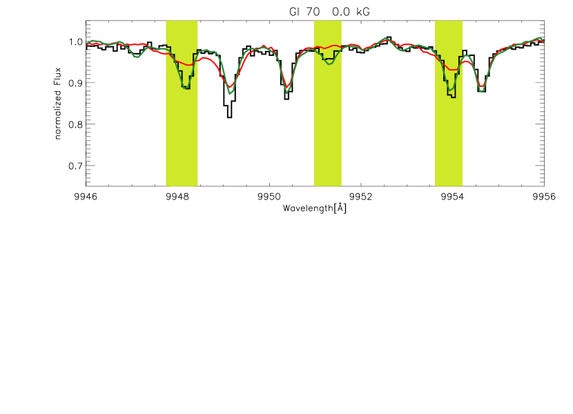
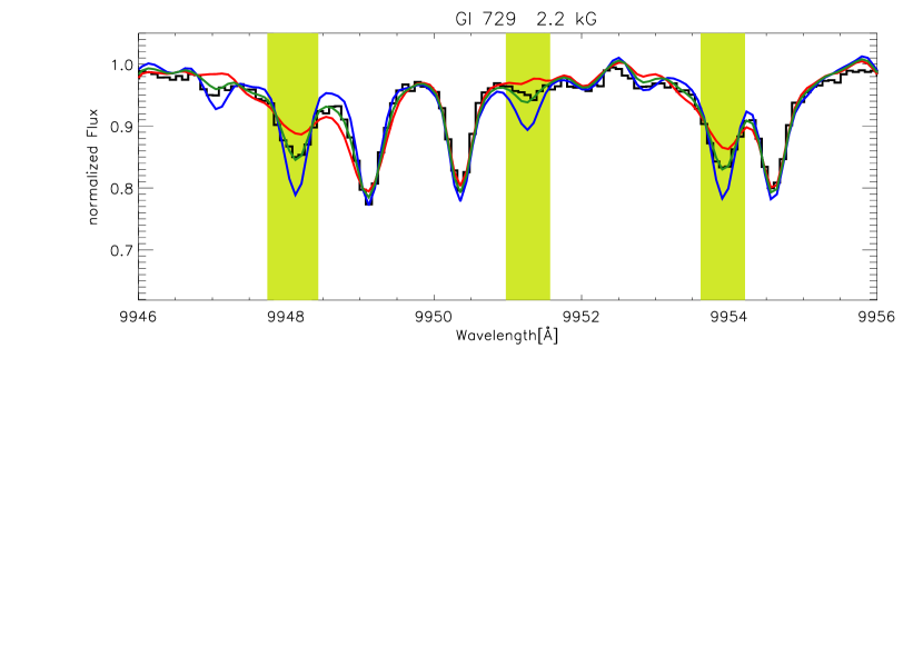
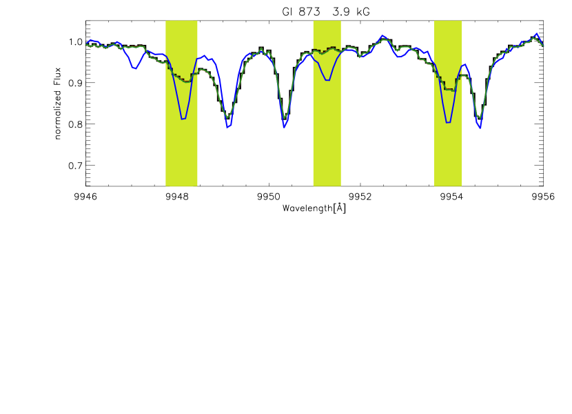
Figure 1: A section of the fits to Gl 70 (M2), Gl 729 (M3.5), and Gl 873 (M3.5). In all plots the case of no magnetic flux is shown in blue, strong magnetic flux ($\sim$4 kG) in red, and the best fit is overplotted in green with the actual value of $Bf$ given above the plots. The green bars indicate parts of the spectrum that are particularly sensitive to the presence of a magnetic field. There is no red line for Gl 873 because the green line is coincident with it.

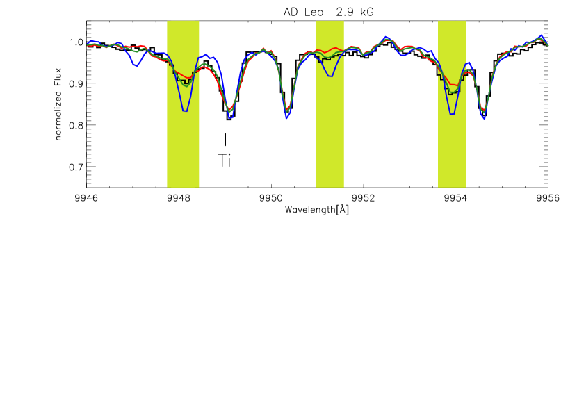
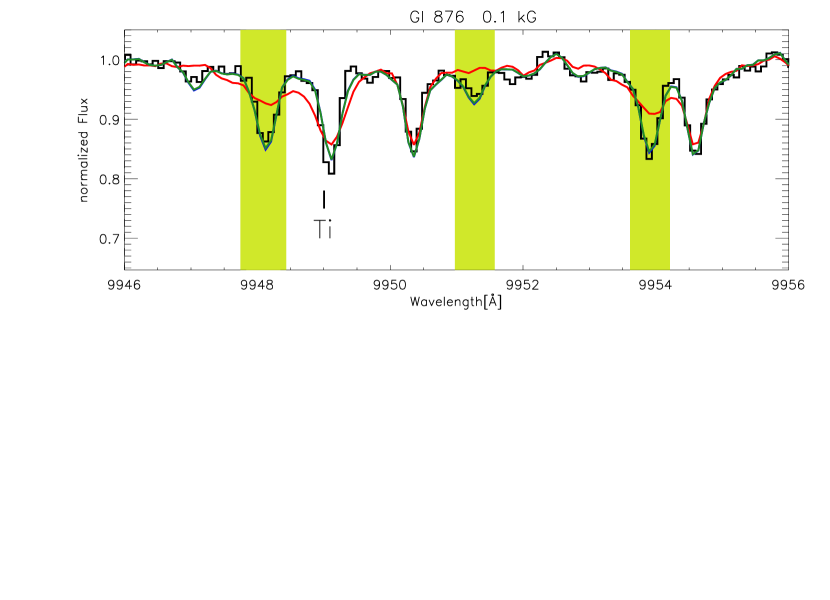
Figure 2: Same as Fig. 1 for AD Leo (M3.5), Gl 876 (M4), and GJ 1005A (M4).

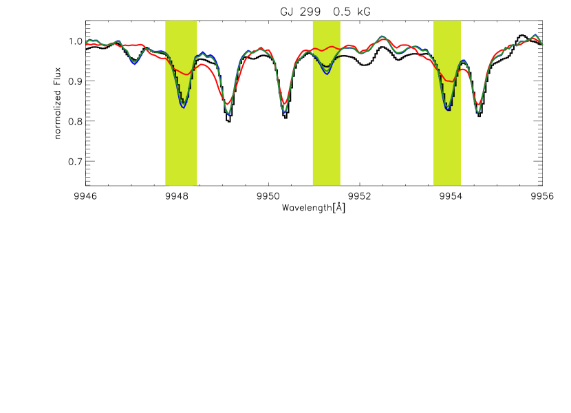
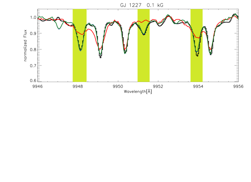
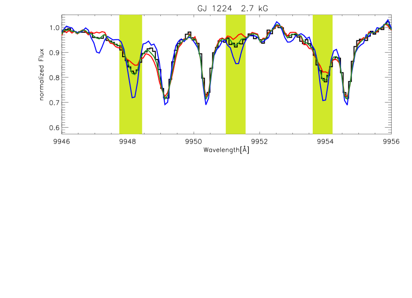
Figure 3: Same as Fig. 1 for Gl 299 (M4.5), GJ 1227 (M4.5), and GJ 1224 (M4.5).

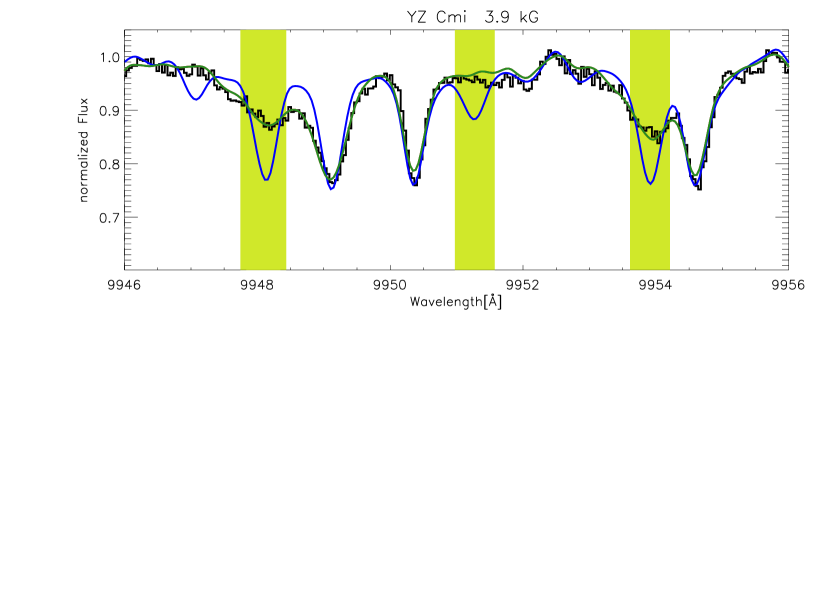
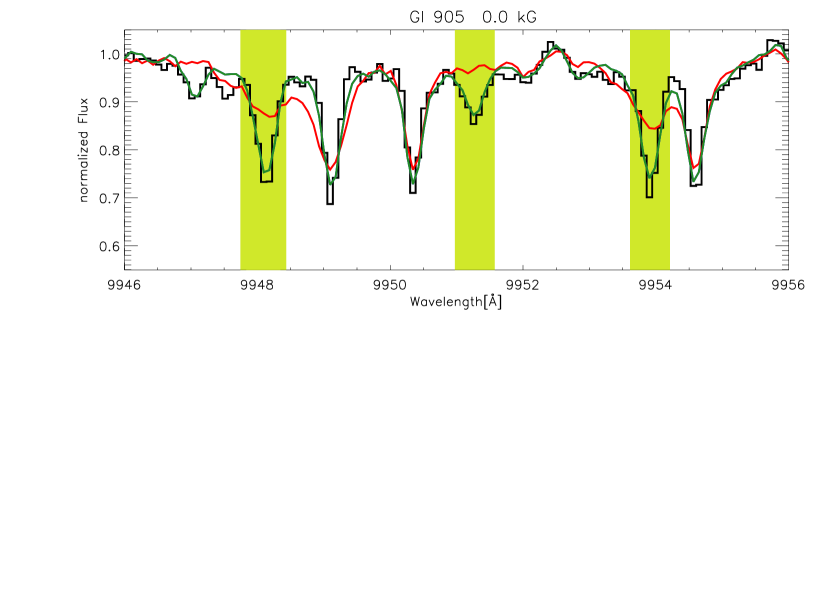
Figure 4: Same as Fig. 1 for YZ Cmi (M4.5), Gl 905 (M5), and GJ 1057 (M5).

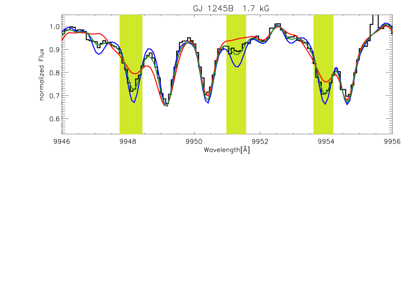
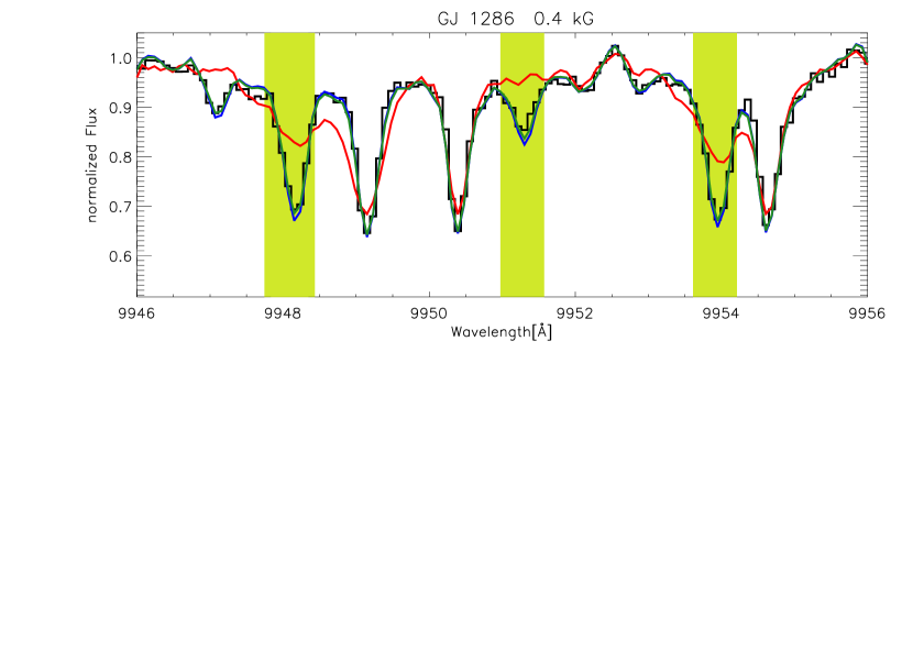
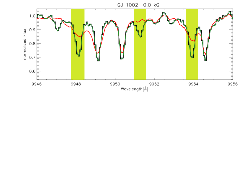
Figure 5: Same as Fig. 1 for GJ 1245AB (M5.5), GJ 1286 (M5.5), and GJ 1002 (M5.5).

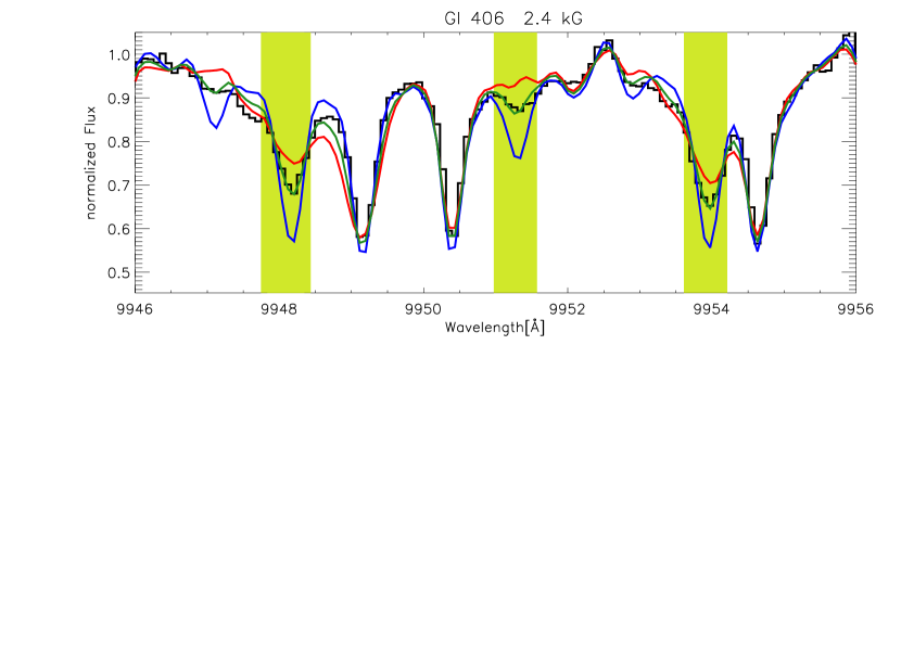
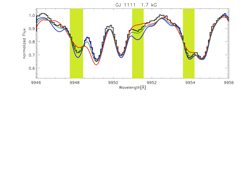
Figure 6: Same as Fig. 1 for Gl 406 (M5.5), GJ 1111 (M6), and VB 8 (M7)

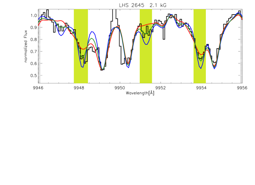
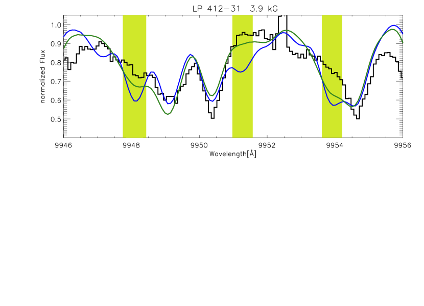
Figure 7: Same as Fig. 1 for LHS 3003 (M7), LHS 2645 (M7.5), and LP 412$-$31 (M8). There is no red line in the bottom panel because the green line is coincident with it.

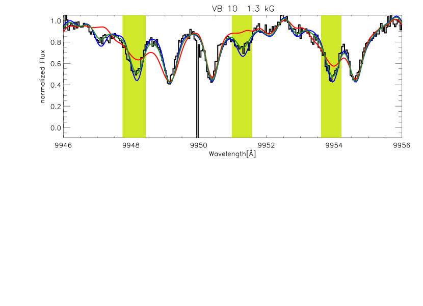
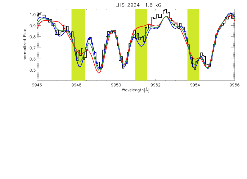
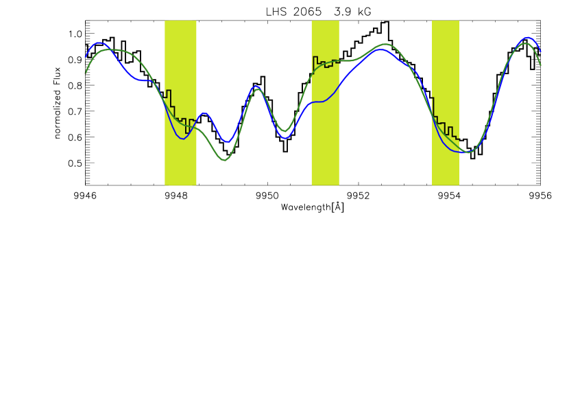
Figure 8: Same as Fig. 1 for VB 10 (M8), LHS 2924 (M9), and LHS 2065 (M9). There is no red line in the bottom panel because the green line is coincident with it.

The results of our spectral analysis are summarized in Table 3. For all targets, projected rotation velocity $v\,\sin{i}$, FeH strength $a$, and H$\alpha$ activity in terms of log ($L_{\rm H\alpha}/L_{\rm bol}$) are given. Literature values of X-ray activity log ($L_{\rm X}/L_{\rm bol}$) are included where available. We analyzed the spectra of 24 objects of spectral types between M2 and M9; they cover the temperature region between 2400 and 3600 K. The two stars Gl 873 (M3.5) and GJ 1002 (M5.5) were used as reference objects. For each object, the wavelength region 9946 – 9956 Å, which is one of the four regions we used for the fitting procedure, is shown in Figs. 1 – 8. In these plots, data is plotted in black, the best fit is overplotted as a green line. Additionally, we show the pure enhanced and rotationally broadened spectra of GJ 1002 and Gl 873, i.e. the two bracketing extremes of zero field strength and a field of $Bf\approx 4$ kG in blue and red color, respectively. Three lines that are particularly sensitive to magnetic splitting are indicated with light green bars. Here the signature of magnetic broadening is most obvious. Several magnetically insensitive lines show how lines are broadened without the influence of magnetic fields, i.e. the broadening predominantly due to rotation.

In the spectrum of some of the warmer objects, (Gl 70, AD Leo, Gl, 876, and GJ 1005A), the Ti line at 9949 Å causes a difference with the template spectra, so we excluded the Ti line from the fit. In all cases, the quality of the fit in the magnetically insensitive lines shows that the rotation velocity cannot be higher than in the achieved fit, and the magnetically sensitive lines allow us to reliably distinguish between weak or zero field strength, intermediate field strength, and strong fields.

In two targets, LP 412-31 and LHS 2065, the best solution does not accurately reproduce the target spectra, but instead appears to require a stronger field than our high-field standard. In them, rotational broadening is above 10 km s^-1 and FeH absorption is very strong, so that saturation and rotational broadening wash out the structure of individual FeH lines. Furthermore, data quality in these faint targets is not as high as in the earlier M-type stars. We show the spectra of LP 412-31 and LHS 2065 in the lower panels of Figs. 7 and 8, respectively. The best fits come from the enhanced and rotationally broadened spectrum of Gl 873 (i.e., $p=1$ in Eq. 1), but it does not convincingly match the data in both spectra. On the other hand, both spectra show a behavior that is much closer to the strong-field case (the green line sits on top of the red line) than to the weak-field case (blue) especially in the magnetically sensitive regions. In the case of LP 412-31, the spectrum even seems to be a natural extrapolation of the sequence of spectra from the blue (no field) over the green ($Bf\approx 4$ kG) spectrum towards the observed data. Based on this we suggest that the magnetic flux $Bf$ in LP 412-31 is substantially higher than on Gl 873, i.e. that the filling factor $f$ is larger than on Gl 873. The mean field in LHS 2065 seems to be only slightly stronger than the 4 kG in Gl 873. As a consistency check, we used the method of line ratios as explained in Paper I, where we measured ratios of two neighbored lines, of which one is magnetically sensitive and the other is magnetically insensitive. From the pair at 9948/9950 Å we derive ratios consistent with a minimum flux of 3.9 kG in both targets. The values from the pairs at 9954/9955 Å exceed the valid range of that ratio and also suggest a field strength in excess of the one in Gl 873.

4.1 Rotation velocities

The rotation velocities of our objects are presented in the fourth column of Table 3. We think that the rotation velocities derived from the FeH band adjusted for spectral type may be superior to those derived from comparison to warmer templates for two reasons: (a) the modification of the FeH strength provides a template that much better reproduces the unbroadened spectrum of VLMS than an uncorrected spectrum of a slowly rotating M-type dwarf does, and (b) the structural richness of the FeH band gives a clearer signal than most other regions in the spectra do. This will be even more important for the analysis of L-dwarfs.

For LHS 3003 we are not aware of any determination of $v\,\sin{i}$ in the literature. All other measurements are consistent with the values we found in the literature except for AD Leo (discussed below). All the objects later than M6 show detectable rotation.

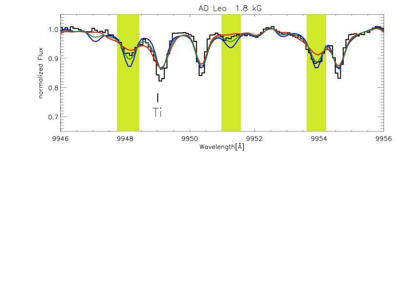
Figure 9: Same as upper panel in Fig. 2 (AD Leo, M3.5) but with $v\,\sin$ fixed at 6 km s^-1.

Vogt et al., (1983); Marcy & Chen, (1992); Delfosse et al., (1998) and Fuhrmeister et al., (2004) spectroscopically measured $v\,\sin{i}$ in AD Leo and all report rotation of $v\,\sin{i}=5-7$ km s^-1. We show the best fit that we can achieve with a value of $v\,\sin{i}=6$ km s^-1 in Fig. 9 in the same manner as in the previous plots. For this case, the magnetic flux we derive is diminished (only 1.8 kG instead of 2.9 kG) compared to our best fit. The fit quality, however, is worse, particularly in the Zeeman-insensitive lines at $\lambda=9950.3$ and 9954.6 Å, which are clearly too broad in the fit compared to the data. We thus think that the projected rotation velocity of AD Leo is around 3 km s^-1 rather than 6 km s^-1. We obtain similar results from our own more careful cross-correlation analysis in selected TiO regions. The rotation period of AD Leo has been suggested to be 2.7 days from photometric variability (Spiesman & Hawley,, 1986), which would produce an equatorial rotation velocity of around 10  km s^-1 (and therefore suggest that we are viewing it at a low inclination angle).

4.2 Magnetic fields

We present our measurements of integrated magnetic flux in the last column of Table 3. These results comprise the first direct detections of magnetic fields in objects later than M4.5; they suggest that magnetic fields are ubiquitous in late-type dwarfs at least down to spectral type M9. The M8 object LP 412-31 and the M9 object LHS 2065 appear to exhibit magnetic flux $Bf$ that are probably stronger than in any other of our targets, which otherwise have values of $Bf$ less than or on the order of 3-4 kG.

Our results on the magnetic fluxes are plotted as function of spectral type and projected rotation velocity in the left and right panels of Fig. 11. In the left panel of Fig. 11 we indicate the rotation velocity of the targets using large symbols for (relatively) rapid rotators. In the right panel, stars cooler than $T_{\rm eff}=2600$ K are plotted as filled triangles, stars warmer than $T_{\rm eff}=3000$ K as filled circles, and intermediate stars near to spectral type M7 are plotted as open squares. For the following, we call a mean field on the order of $Bf\sim 2$ kG an intermediate field, and a mean field on the order of $Bf\sim 4$ kG a strong field. Note that for solar-type stars, a flux of $Bf\sim 2$ kG would be considered a strong field (even in K-type T Tauri stars).

Both panels in Fig. 11 show that strong and intermediate magnetic fields occur at the whole range of spectral types and rotation velocities covered by our sample. In our early-type M dwarfs (M2-3.5), the situation is not clear-cut. AD Leo is a famous flare star but doesn’t show much rotational broadening. Gl 873 similarly has strong H$\alpha$ emission and high magnetic flux but very low rotational broadening. Gl 729 shows both rotation and a field; Gl 70 and Gl 876 show neither. This sample is too small, and should be increased (although finding measurable rotators at this spectral type is not easy). The total number of actual field measurements for the (most easily observed) early M dwarfs is rather sparse (and confined to dMe stars). Almost all of the sample in Delfosse et al., (1998) are too slowly rotating to show broadening, but that makes it easier to detect field effects. Clearly, more research should be conducted in this part of parameter space.

Among the M4-5.5 stars there are 3 measurable rotators (although with only a marginal detection in the case of Gl 406), all of which show fields (the most active is the famous flare star YZ CMi). One slower rotator also shows fairly strong flux and activity (GJ 1224); again there is the possibility that inclination is making the rotational broadening small in this case. Otherwise the 8 slow rotators have no field detected. This appears to be reasonable evidence for a rotational influence. It has already been noted by Mohanty & Basri, (2003), though using proxies instead of actual flux measurements.

We find no clear relation between rotation velocity and mean magnetic field in our late-M sample. Instead, all cool objects exhibit detectable magnetic flux. No rotation-activity relation was found in very late objects (Mohanty & Basri,, 2003), so we did not expect a dependence between $v\,\sin{i}$ and $Bf$ in objects later than $\sim$ M7. However, the two cases in which we detect a very strong mean field are rapid rotators with $v\,\sin{i}>10$ km s^-1. This could indicate a dependence of field generation on rotation at late spectral types of some sort, but such a suggestion is hampered by the lack of slowly rotating late-M objects in general (which would help define it), and certainly is not statistically significant in our sample. It is also worth noting that the filling factor is thought to be near unity for dMe stars (or T Tauri stars), so it is likely that the field strength itself is greater in these very strong objects.

Noyes et al., (1984) pointed out the potential relevance of Rossby number ($P_{rot}/\tau_{c}$) to the production of magnetic fields in convective dynamos, where $\tau_{c}$ is the convective overturn timescale and $P_{rot}$ is the rotational period. Mohanty & Basri, (2003) did not find strong evidence that it matters for fully convective stars. Whether the Rossby number is relevant or not depends in part on the length scale at which the field is produced, and whether it is large enough to let rotation play a role. We now have a chance to further probe this question. A crude estimate for $\tau_{c}$ in fully convective stars can be derived as follows. An expression for convective velocities in mixing length theory is ${v_{c}}^{3}\propto({{\Gamma-1}\over\Gamma}){L_{*}\over{{R_{*}}^{2}\rho}}$ (Thompson & Duncan,, 1993). Since these objects are fully convective, we can take the convective luminosity to be the stellar luminosity, the radius to be the stellar radius, and the density to be the mean stellar density. For very low-mass stars, radius scales like mass. Luminosity is often assumed to behave like $M^{\beta}$. Then we find ${v_{c}}^{3}\propto{{L_{*}R_{*}}\over M_{*}}\rm{\ \ \ or\ \ \ }v_{c}\propto{M_{*}}^{\beta/3}.$ The first of these two results can also be obtained from a dimensional analysis. Since the convective overturn time can likewise be approximated as $\tau_{c}\propto{R_{*}/v_{c}}$; we find that $\tau_{c}\propto{M_{*}}^{1-(\beta/3)}$.

Often $\beta$ is taken to be roughly 5 for this mass range, in which case $\tau_{c}$ is inversely proportional to ${M_{*}}^{(2/3)}$. The situation is actually somewhat more complicated (even if we simplify by restricting ourselves to talking about objects several Gyr old). To estimate $\beta$ we used the models of Chabrier et al., (2000) and looked at gradients in luminosity over small increments of mass. Above and near the fully convective boundary $\beta\approx 3$ (which makes $\tau_{c}$ almost constant), but then it becomes very steep towards the substellar boundary, reaching values of several tens. This means that the convective overturn times grow quite long near the substellar boundary (where degeneracy is taken over from fusion). That is exaggerated further by the fact that radius is no longer linear in mass, as degeneracy causes it to become nearly constant (then depend inversely on mass). The rotation periods also vary greatly over the mass range of interest (from weeks for inactive early-M stars to days for active mid-M stars to hours for late-M stars). Rotation must therefore be the driving force behind any dependence on Rossby number for stars above about two-tenths of a solar mass, but convection is probably more important at the bottom of the main sequence. What is clear is that both the longer convective overturn times and increasingly rapid rotations of the very cool objects push the Rossby numbers to very small values. This obviously does not hamper the generation of strong, widespread fields, however. That is a valuable clue for the study of fully convective dynamos.

4.3 H$\alpha$ activity and magnetic flux

Our measurements of activity from H$\alpha$ and of the magnetic flux are derived from the same spectrum. We can thus directly investigate the dependence of H$\alpha$ activity on the magnetic field even though both may well be variabler. We plot our measurements of activity in terms of the ratio of the luminosity in H$\alpha$ to the bolometric luminosity, log $L_{\rm H\alpha}/L_{\rm bol}$, as a function of spectral type in the left panel of Fig. 12. Symbols indicate magnetic flux as explained in the caption. This plot resembles Fig. 7 from Mohanty & Basri, (2003) and confirms their findings; in the stars earlier than M7, activity measurements span a range of at least two magnitudes with several non-detections. All objects of spectral types M6 – M9 show significant H$\alpha$ emission (no lower limits), and a steep fall-off in log $L_{\rm H\alpha}/L_{\rm bol}$ is observed towards the coolest objects as in Gizis et al., (2000) and West et al., (2004). Among the active stars only, the level of activity is continually decreasing towards later spectral type.

In the same plot, we indicate magnetic field strengths by different symbols. For each spectral type, the highest value of log $L_{\rm H\alpha}/L_{\rm bol}$ is measured in the stars with the strongest fields, and all inactive stars have weak (or no) magnetic fields. This means that at given spectral type log $L_{\rm H\alpha}/L_{\rm bol}$ correlates with magnetic flux. The plot of log $L_{\rm H\alpha}/L_{\rm bol}$ as a function of magnetic flux $Bf$ in the right panel of Fig. 12 demonstrates this relation (we use the same symbols as before in the right panel of Fig. 11).

Among the two groups of stars that have temperatures warmer than 3000 K (full circles) and cooler than 2600 K (full triangles), the measured level of activity is proportional to the magnetic flux $Bf$ among the stars that show H$\alpha$ emission. All non-active stars have weak or zero field strength. It can also be seen that activity drops towards later spectral type, i.e. there is an offset between the two groups. Three targets are of intermediate temperature (spectral type $\sim$ M7), and they fall between the two groups of warm and cool objects. We describe the relations among the warm and the cool objects by independently fitting a linear model to the active stars in these groups. The relations are overplotted in the right panel of Fig. 12 as dotted lines, they are best approximated by the following parameterizations:

$$\mathrm{earlier~{}than~{}M7} : \mathrm{log}\frac{L_{\mathrm{H}\alpha}}{L_{\mathrm{bol}}}=-4.26+0.22Bf$$ (2)

$$\mathrm{later~{}than~{}M7} : \mathrm{log}\frac{L_{\mathrm{H}\alpha}}{L_{\mathrm{bol}}}=-5.03+0.27Bf$$ (3)

If we assume an uncertainty in the measurement of the magnetic flux of $\Delta Bf=1$ kG, we formally derive correlation coefficients of $(0.22\pm 0.07)$ and $(0.27\pm 0.16)$ for the two subsamples. The dependence of log $L_{\rm H\alpha}/L_{\rm bol}$ on $Bf$ appears to be similar in both groups, although a flatter slope for the cooler group might result if we had an actual value for LP 412-31. The fact that the three objects of intermediate temperature fall between the two relations indicates a continuous dependence of $Bf$ on spectral type rather than an abrupt change at spectral type M7.

All the objects M6 or later show detectable rotation and also H$\alpha$ emission. Those with rotations similar to the M4.5-5.5 rotators of 5-10 km s^-1 (namely VB 8 and 10, LHS 3003 and 2645, GJ 1002) have intermediate fluxes (the comparable mid-M stars are intermediate or strong), while those above 10 km s^-1 have very strong fields (LP 412-31 and LHS 2065). Even in these two cases, however, the H$\alpha$ emission is not as strong as for any of the mid-M rotators. One star rotates pretty rapidly and has an intermediate flux, but does not have as strong activity (GJ 1111); it is at the warm end of this subset (M6). This may mark the beginning of the weakening of the field-activity connection with falling photospheric temperature. That is the effect predicted to result from increasing atmospheric neutrality (which decouples the field from atmospheric motions), although it is at a little warmer temperature than models suggest. This is consistent with what was found by West et al., (2004), who also found that not all late-M stars showed H$\alpha$ emission. It would be good to try to observe a few such inactive stars to determine whether they are also slow rotators, and do not show detectable fields.

There appears to be no reason to imagine that the L dwarfs (at least the early-type ones) are inactive due to an inability to generate fields. That is consistent with the inference of fields on L dwarfs by (Berger et al.,, 2005; Berger,, 2006). Our suggested trend of increasing field at later spectral types, however, is somewhat opposite of the impression one gets from Fig. 2 of Berger, (2006), although in both cases the samples of field detections are too small for clear conclusions. We note that our field detections are much more direct than those inferred from gyrosynchrotron radio emission by Berger, (2006); ours refer directly to the stellar surface rather than a radio-emitting region well above the star and require no assumptions about electron-density power spectrum, or emitting-region geometry. We are therefore able to conclude that rather strong fields exist in the photosphere, contrary to the tentative conclusion those authors make that the fields may be somewhat weaker than in earlier M dwarfs.

5 Conclusions

This is the first attempt to measure magnetic fields directly on stars with effective temperatures below 3200K. At these temperatures the objects are firmly in the fully convective regime, so one is studying dynamo action of the sort that is probably most common in stars and disks (the cyclical solar dynamo is thought to operate only at radiative-convective interfaces). We find evidence that the increasingly small Rossby numbers near the bottom of the main sequence are no hindrance to the generation of magnetic flux.

The sample of stars in this study is too small and biased to draw general conclusions from it. We offer several conjectures supported by our results that can be followed up by more work using our new methodology. These are: 1) magnetic fields exist, and can be quite strong, throughout the M spectral sequence; 2) there may be a connection between the rotation of the star and the amount of flux it produces, although it is not yet clearly known what it is (and how saturation plays a role in it); 3) there is a correlation between the magnetic flux and the fractional amount of H$\alpha$ emission observed when such emission is seen; 4) there is evidence that the fractional amount of H$\alpha$ emission falls with photospheric temperatures in late-M dwarfs regardless of how much magnetic flux they have, supporting the proposition that activity fades at the bottom of the M-sequence due to atmospheric neutrality rather than a fall in magnetic flux production.

One of the most pressing questions left unanswered by this initial work is whether we can actually measure fields on early L-dwarfs even though they rarely exhibit emission activity. These objects are more challenging for our method because of the heavy saturation of the FeH lines, and the great tendency for rapid rotation in these objects. The latter problem is almost certainly due to a lack of magnetic braking, but it remains unresolved whether it is the field itself or its coupling to the upper atmosphere that is to blame. Another current mystery is why very young objects in the late-M spectral range appear to be substantially more active than older objects of the same temperature. That is a surprising result if the dominant effect turning activity off in the very low-mass field objects is atmospheric neutrality (which depends on temperature). Is this difference in activity due to different magnetic flux generation at different ages, or some other characteristic (eg. low gravity or primordial fields) in younger objects? This question is more easily attacked with our current methodology, and we have already begun observations to address it.

Table 1: Table of targets, exposure times and SNR measured in the FeH band

Name	SpT	$J$ mag	exposure [s]	SNR
Gl 70	M2.0	07.37	0300	150
Gl 729	M3.5	06.22	0120	145
Gl 873	M3.5	06.11	0120	140
AD Leo	M3.5	05.45	0120	100
Gl 876	M4.0	05.93	0120	085
GJ 1005A	M4.0	07.22	0240	090
Gl 299	M4.5	08.42	1200	065
GJ 1227	M4.5	08.64	1200	075
GJ 1224	M4.5	08.64	0600	075
YZ Cmi	M4.5	06.58	0600	070
Gl 905	M5.0	06.88	0180	060
GJ 1057	M5.0	08.78	0300	060
GJ 1245B	M5.5	08.28	0300	070
GJ 1286	M5.5	09.14	0600	050
GJ 1002	M5.5	08.32	0300	065
Gl 406	M5.5	07.09	0200	060
GJ 1111	M6.0	08.24	0600	050
VB 8	M7.0	09.78	0600	040
LHS 3003	M7.0	09.97	0600	035
LHS 2645	M7.5	12.19	2000	030
LP 412$-$31	M8.0	11.76	2400	030
VB 10	M8.0	09.91	1100	025
LHS 2924	M9.0	11.99	1800	020
LHS 2065	M9.0	11.21	1200	035

Table 2: Spectral regions used for the fit

Slow rotators
9895.5	–	9905.5 Å
9937.5	–	9941.0 Å
9946.0	–	9956.0 Å
9974.5	–	9978.0 Å
Rapid rotators
9920.0	–	9926.0 Å
9932.0	–	9937.0 Å
9946.0	–	9952.0 Å
9977.5	–	9982.0 Å

Table 3: Results from our analysis. Effective temperature is from the calibration of Golimowski et al., (2004), X-ray luminosities are from the literature as indicated. We give formal 2$\sigma$ uncertainties for $Bf$, but we note that total uncertainties are on the order of a kilo-Gauss (see text).

Name	Sp	$T_{\rm eff}$	$v\,\sin{i}$	FeH $a$	H$\alpha$ EqW	log($\frac{L_{\mathrm{H\alpha}}}{L_{\mathrm{bol}}}$)	log($\frac{L_{\mathrm{X}}}{L_{\mathrm{bol}}}$)	$Bf_{\rm fit}$
		[K]	[km s-1]		[Å]			[kG]
Gl 70	M2.0	3580	$\leq$3	0.5	$<0.20$	$<-4.91$	$<-4.44$	$<0.1$
Gl 729	M3.5	3410	4	1.1	$4.47$	$-3.66$	$-3.50$	$2.2\pm 0.1$
Gl 873	M3.5	3410	$\leq$3	0.9	$5.98$	$-3.53$	$-3.07$	$3.9$
AD Leo	M3.5	3410	$\approx$3	0.8	$3.40$	$-3.78$	$-3.02$	$2.9\pm 0.2$
Gl 876	M4.0	3360	$\leq$3	0.7	$<0.21$	$<-4.97$	$-5.23$	$<0.2$
GJ 1005A	M4.0	3360	$\leq$3	0.8	$<0.21$	$<-4.95$	$-5.05$	$<0.1$
GJ 299	M4.5	3300	$\leq$3	0.8	$<0.33$	$<-4.84$	$<-5.55$	$0.5\pm 0.2$
GJ 1227	M4.5	3300	$\leq$3	1.0	$<0.32$	$<-4.85$	$<-3.86$	$<0.1$
GJ 1224	M4.5	3300	$\leq$3	1.4	$4.13$	$-3.74$	$-3.06$	$2.7\pm 0.1$
YZ Cmi	M4.5	3300	5	1.2	$8.42$	$-3.43$	$-3.02$	$>3.9$
Gl 905	M5.0	3240	$\leq$3	1.2	$<0.30$	$<-4.95$	$-3.75$	$<0.1$
GJ 1057	M5.0	3240	$\leq$3	1.2	$1.06$	$-4.41$	$<-3.87$	$<0.2$
GJ 1245B	M5.5	3150	7	2.1	$4.26$	$-3.76$	$-3.58$	$1.7\pm 0.2$
GJ 1286	M5.5	3150	$\leq$3	1.7	$1.50$	$-4.21$	$<-3.77$	$0.4\pm 0.2$
GJ 1002	M5.5	3150	$\leq$3	1.5	$<0.36$	$<-4.83$	$<-5.24$	$0.0$
Gl 406	M5.5	3150	3	2.6	$9.93$	$-3.39$	$-2.77$	$2.4\pm 0.1$
GJ 1111	M6.0	2840	13	2.8	$8.12$	$-3.92$	$-3.88$	$1.7\pm 0.2$
VB 8	M7.0	2620	5	3.4	$7.09$	$-4.27$	$-3.47$	$2.3\pm 0.2$
LHS 3003	M7.0	2620	6	3.3	$7.60$	$-4.24$	$-4.01$	$1.5\pm 0.2$
LHS 2645	M7.5	2540	8	3.1	$4.26$	$-4.67$		$2.1\pm 0.2$
LP 412$-$31	M8.0	2480	9	4.0	$23.05$	$-3.89$		$>3.9$
VB 10	M8.0	2480	6	4.2	$6.53$	$-4.44$	$-4.9$	$1.3\pm 0.2$
LHS 2924	M9.0	2390	10	4.3	$5.76$	$-4.70$	$-4.35$	$1.6\pm 0.2$
LHS 2065	M9.0	2390	12	4.6	$29.05$	$-4.00$	$-3.50$	$>3.9$

Figure 10: $L_{\alpha}/L_{\mathrm{bol}}$ vs. $L_{\mathrm{X}}/L_{\mathrm{bol}}$

Figure 11: Left panel: Magnetic flux $Bf$ vs. spectral type; the size of the symbols scales with projected rotation velocity $v\,\sin{i}$. Right panel: $Bf$ vs. $v\,\sin{i}$, three groups of effective temperature $T_{\rm eff}$ are distinguished by different symbols as indicated in the plot. In both panels, up- and downward arrows indicate upper and lower limits in $Bf$, respectively.

Figure 12: Normalized H$\alpha$ luminosity log $L_{\rm H\alpha}/L_{\rm bol}$. Left panel: log $L_{\rm H\alpha}/L_{\rm bol}$ vs. spectral type, symbols distinguish objects with weak or no magnetic flux, intermediate flux, and strong flux as shown in the plot. Right panel: log $L_{\rm H\alpha}/L_{\rm bol}$ vs. $Bf$. Symbols indicate temperature as in the right panel of Fig. 11.

References

- Allard et al., (2001) Allard, F., Hauschildt, P.H., Alexander, D.R., Tamanai, A., & Schweitzer, A., 2001, ApJ, 556, 357
- Bailer-Jones, (2004) Bailer-Jones, C.A.L., 2004, A&A, 419, 703
- Basri & Marcy, (1995) Basri, G., Marcy, G.W. 1995, AJ, 109, 762
- Basri et al., (2000) Basri, G., Mohanty, S., Allard, F., Hauschildt, P.H., Delfosse, X., Martín, E.L., Forveille, T., & Goldman, B., 2000, ApJ, 538, 337
- Berger et al., (2005) Berger, E., Rutledge, R.E., Reid, I. N., Bildsten, L., Gizis, J.E., Liebert, J. and 9 coauthors 2005, ApJ, 627, 960
- Berger, (2006) Berger, E. 2006, astro-ph 0603176
- Chabrier et al., (2000) Chabrier, G., Baraffe, I., Allard, F., Hauschildt, P. 2000, ApJ, 542, 464
- Delfosse et al., (1998) Delfosse, X., Forveille, T., Perrier, C., & Mayor, M., 1998, A&A, 331, 581
- Durney et al., (1993) Durney, B.R., De Young, B.S., & Roxburgh, I.W., 1993, Sol.Phys., 145, 207
- Dobler et al., (2006) Dobler, W., Stix, M., & Brandenburg, A., 2006, ApJ, 638, 336
- Donati et al., (2006) Donati, J.-F. Forveille, T., Cameron-Collier, A., Barnes, J. R., Delfosse, X. Jardine, M. M., Valenti, J. A. 2006, Science, 311, 633
- Fleming et al., (1993) Fleming, T.A., Giampapa, M.S., Schmitt, J.H.M.M., and Bookbinder, J.A., 1993, ApJ, 410, 387
- Fleming et al., (1995) Fleming, T.A., Schmitt, J.H.M.M., and Giampapa, M.S., 1995, ApJ, 450, 401
- Fleming et al., (2003) Fleming, T.A., Giampapa, M.S., and Garza, D., 2003, ApJ, 594, 982
- Fuhrmeister et al., (2004) Fuhrmeister, B., Schmitt, J.H.M.M., & Wichmann, R., 2004, A&A, 417, 701
- Gizis et al., (2000) Gizis, J.E., Monet, D.G., Reid, I.N., Kirkpatrick, J.D., Liebert, J., Williams, R.J. 2000, AJ, 120, 1085
- Gliese & Jahreiss, (1991) Gliese, W., & Jahreiss, H., 1991, Third Catalogue of Nearby Stars (Heidelberg: Astron. Rechen Inst.)
- Golimowski et al., (2004) Golimowski, D.A., Leggett, S.K., Marley, M.S., et al., 2004, AJ, 127, 3516
- Johns-Krull & Valenti, (1996) Johns-Krull, C., & Valenti, J.A., 1996, ApJ, 459, L95
- Johns-Krull & Valenti, (2000) Johns-Krull, C., & Valenti, J.A., 2000, ASPC, 198, 371
- Kenyon & Hartmann, (1995) Kenyon, S.J., & Hartmann, L., 1995, ApJS, 101, 117
- Marcy & Chen, (1992) Macry, G.W., & Chen, G.H., 1992, ApJ, 390, 550
- Mohanty et al., (2002) Mohanty, S., Basri, G., Shu, F., Allard, F., & Chabrier, G. 2002, ApJ, 571, 469
- Mohanty & Basri, (2003) Mohanty, S., & Basri, G., 2003, ApJ, 583, 451
- Press et al., (1992) Press W.H., Teukolsky S.A., Vetterling W.T., and Flannery B.P., 1992, Numerical Recipes in C, Cambridge Universtity Press
- Noyes et al., (1984) Noyes, R.W., Hartmann, L.W., Baliunas, S.L., Duncan, D.K., Vaughan, A.H. 1984, ApJ, 279, 763
- (27) Reiners, A., & Basri, G., ApJ, 644, 497 (Paper I)
- (28) Reiners, A., & Basri, G., AJ, 131, 1806
- Saar, (2001) Saar, S. 2001, ASP-CS, 233, 292
- Schmitt & Liefke, (2004) Schmitt, J.H.M.M., & Liefke, C., A&A, 417, 651
- Schweitzer et al., (1996) Schweitzer, A., Hauschildt, P.H., Allard, F., Basri, G. 1996, MNRAS, 283, 821
- Spiesman & Hawley, (1986) Spiesman, W. J., Hawley, S. L. 1986, AJ, 92, 664
- Thompson & Duncan, (1993) Thompson, C. & Duncan, R.C. 1993, ApJ, 408, 194
- Vogt et al., (1983) Vogt, S.S., Soderblom, D.R., & Penrod, G.D., 1983, ApJ, 269, 250
- West et al., (2004) West, A.A., Hawley, S.L., Walkowicz, L.M., Covey, K.R., Silvestri, N.M., and 6 authors 2004, AJ, 128, 426