Systematic errors in cosmic microwave background polarization measurements

Abstract

We investigate the impact of instrumental systematic errors on the potential of cosmic microwave background polarization experiments targeting primordial $B$-modes. To do so, we introduce spin-weighted Müller matrix-valued fields describing the linear response of the imperfect optical system and receiver, and give a careful discussion of the behaviour of the induced systematic effects under rotation of the instrument. We give the correspondence between the matrix components and known optical and receiver imperfections, and compare the likely performance of pseudo-correlation receivers and those that modulate the polarization with a half-wave plate. The latter is shown to have the significant advantage of not coupling the total intensity into polarization for perfect optics, but potential effects like optical distortions that may be introduced by the quasi-optical wave plate warrant further investigation. A fast method for tolerancing time-invariant systematic effects is presented, which propagates errors through to power spectra and cosmological parameters. The method extends previous studies to an arbitrary scan strategy, and eliminates the need for time-consuming Monte-Carlo simulations in the early phases of instrument and survey design. We illustrate the method with both simple parametrized forms for the systematics and with beams based on physical-optics simulations. Example results are given in the context of next-generation experiments targeting tensor-to-scalar ratios $r\sim 0.01$.

1 Introduction

There is currently a great deal of interest and activity in the field of cosmic microwave background (CMB) polarimetry. Several recent experiments (Kovac et al., 2002; Readhead et al., 2004; Barkats et al., 2005; Montroy et al., 2006; Page et al., 2006; Wu et al., 2007) have reported detections of CMB polarization at a level consistent with predictions in simple cold dark matter (plus $\Lambda$) models fit to the temperature anisotropy data. In standard adiabatic models, polarization measurements promise a further tightening of constraints inferred from the temperature anisotropies, and the breaking of important degeneracies (Zaldarriaga, Spergel & Seljak, 1997). In particular, with the recent release of the three-year Wilkinson Microwave Anisotropy Probe (WMAP) data, the optical depth to reionization has been constrained to $\tau=0.09\pm 0.03$ (Spergel et al., 2006) with the large-angle polarization signal (Zaldarriaga, 1997). Polarization information is particularly valuable in non-standard models, for example it can significantly improve constraints in the presence of isocurvature modes (Bucher, Moodley & Turok, 2001), and be used to constrain parity-violating physics (e.g. Scannapieco & Ferreira 1997; Lue, Wang & Kamionkowski 1999; Feng et al. 2006). Secondary effects, most notably weak gravitational lensing (Zaldarriaga & Seljak, 1998; Lewis & Challinor, 2006), further encode information on the low-redshift universe in CMB polarization.

Perhaps the most exciting aspect of CMB polarimetry is the window it may open on primordial gravitational waves (Kamionkowski, Kosowsky & Stebbins 1997; Zaldarriaga & Seljak 1997). The curl mode (or $B$-mode) of polarization is not produced by linear density perturbations and so provides an observable signature of gravitational waves at last scattering that is not limited by cosmic variance from the dominant density perturbations. However, the situation is clouded by several issues. First, the amplitude of gravitational waves expected from inflation is unknown as the energy scale at which inflation may have occurred is not (yet) determined by theory. What is known is that any $B$-mode imprint will be very small: the current limit on the amplitude of the gravitational wave power spectrum (expressed as a fraction of that for the density perturbation) is $r<0.28$ at 95% confidence (Spergel et al., 2006), from a combination of the temperature anisotropies and galaxy-clustering data. This limit on $r$ translates to an r.m.s. $B$-mode signal $<200\,\mathrm{nK}$. Furthermore, gravitational lensing does produce $B$-mode polarization at second order in the density perturbations, with a spectrum that is almost white for multipoles $l\la 300$. The amplitude $\sqrt{C^{B}_{l,\mathrm{lens}}}\approx 5\,\mu$K-arcmin means the lens-induced $B$-modes dominate the primordial ones for $r\la 0.01$ except on very large scales where the latter is enhanced by reionization. For noise levels much better than $5\,\mu$K-arcmin, it will be worthwhile to try and clean out the large-angle $B$-modes of lensing by making use of non-Gaussianity (e.g. Hu & Okamoto 2002). Finally, polarized emission from Galactic foregrounds will likely overwhelm the primordial $B$-mode signal over a large fraction of the sky (Page et al., 2006), and our ability to constrain gravitational waves will almost certainly be limited by the accuracy at which Galactic foregrounds can be subtracted.

The intrinsic weakness of the polarization signal presents a major experimental challenge. The gradient (or $E$-mode) polarization is now determined to be at least an order of magnitude smaller than the temperature anisotropies for $l\la 1000$, and the $B$-modes (including lensing) are indirectly constrained to be at least an order of magnitude smaller still. As well as the raw sensitivity requirements that this implies, any systematic errors present in $B$-mode instruments will have to be controlled to an unprecedented level of accuracy in order to ensure the signal is not fatally contaminated. With this motivation, in this paper we develop a general framework to describe and assess the impact of instrumental systematic errors on experiments targeted at CMB polarization.

There is a growing literature discussing the impact of systematic effects in CMB polarimetry; for discussions of the real-world issues encountered in recent surveys, see Barkats et al. (2005); Masi et al. (2006); Page et al. (2006); Jones et al. (2006). There are typically many sources of potential systematic error. Here we shall be concerned with the broad class of errors that produce a time-independent residual signal for a given instrument pointing. These include imperfections in the receiver and optics, but exclude important effects such as low-frequency noise from thermal fluctuations, readout electronics or atmospheric fluctuations, and pointing jitter. Low-frequency noise is best dealt with by a combination of signal modulation (active or by scanning), a well cross-linked survey, and removal during the map-making stage. Our aim is twofold: to give a careful analysis of the transformation properties of various systematic effects under rotation of the instrument – a useful strategy for mitigating some systematics; and to provide a fast, semi-analytic method for tolerancing systematic effects that is flexible enough to deal with arbitrary scan strategies and removes the need for time-consuming simulations during the early stages of instrument and survey design. Our approach is similar to that of Hu, Hedman & Zaldarriaga (2003), but we extend their analysis in several ways. We describe the receiver systematics with Müller matrices and the optics with Müller matrix-valued fields which allows us to deal with arbitrary beam effects. To simplify the discussion of the rotation properties of systematic effects, we introduce spin-weighted Müller matrices and perform a further decomposition of the beam matrix-valued fields into irreducible components. The latter singles out those features of the beams that cannot be overcome with instrument rotation, and easily reproduces the results of Carretti et al. (2004) for axisymmetric systems. In addition, our analysis of the scientific impact of systematic effects works with an arbitrary scan strategy, and propagates the effects through to biases in cosmological parameters and the increase in their random errors. Carrying biases through to parameters is potentially important: systematic errors often must be suppressed further than the cosmic-variance limit in the CMB power spectra if they are to have negligible impact on the science (Efstathiou & Bond, 1999). Also, properly modelling the interaction between systematic effects and the scan strategy is important as its effects cannot easily be predicted, or constrained, from simpler scans (such as a raster scan with no implied beam rotation). For example, a non-trivial scan can cause leakage from the dominant $E$-modes into $B$-modes that is not present for a raster scan, as a result of the non-local nature of the $E$- and $B$-mode decomposition.

This paper is organized as follows. Section 2 introduces our notation and some important assumptions. Propagation through the receiver is described in Section 3 in terms of spin-weighted Müller matrices, while the optics are described in terms of matrix-valued fields in Section 4. We give illustrations for common receiver types and optical imperfections, and compare their relative merits. In Section 5 we present our method for propagating errors to biases in power spectra and the enhancement of their variances, and follow these through to cosmological parameters (specifically $r$) in Section 6. Finally, in Section 7 we apply our methods to set tolerances on parametrized errors and compare these for different scan strategies. We also examine the impact of realistic, simulated beam profiles. Two appendices give further properties of the complex Müller matrices and of the beam expansion in irreducible components introduced in Section 4.

2 Notation

For surveys covering a small fraction of the sky we can work in the flat-sky limit where the CMB fields are considered on the tangent plane to the celestial sphere. We adopt Cartesian coordinates on this plane such that $x$ points north–south and $y$ points west–east; the right-handed $z$-direction is then along the line of sight. We define Stokes parameters using the $x$ and $-y$ directions for which the radiation propagation direction completes a right-handed triad. Our polarization conventions are then consistent with the IAU standards. If the electric field of the incident radiation at frequency $\omega$ is $\Re({\mn@boldsymbol{E}}e^{-i\omega t})$, with these conventions we have

$$\langle E_{i}E_{j}^{*}\rangle=\frac{1}{2}\left(\begin{array}[]{cc}T+Q&-U-iV\\ -U+iV&T-Q\end{array}\right).$$ (1)

We shall only consider quasi-monochromatic systems here but our discussion will still hold for broad-band systems if the non-ideal instrument responds in the same way to all in-band radiation. Clearly this ignores an important class of systematic effects, for example bandpass mismatch (Jarosik et al., 2006).

The complex polarization $P({\mn@boldsymbol{x}})\equiv(Q+iU)({\mn@boldsymbol{x}})$ is spin $-2$ in the sense that under the transformation $\hat{{\mn@boldsymbol{x}}}+i\hat{{\mn@boldsymbol{y}}}\mapsto(\hat{{\mn@boldsymbol{x}}}+i\hat{{\mn@boldsymbol{y}}})e^{i\psi}$, which rotates the $x$-axis by $\psi$ towards the negative $y$-axis, $P\mapsto Pe^{-2i\psi}$. Decomposing $P$ into its electric (E) and magnetic (B) parts, we have, in Fourier space,

$$(Q\pm iU)({\mn@boldsymbol{x}})=-\int\frac{{\mathrm{d}}^{2}{\mn@boldsymbol{l}}}{2\pi}[E({\mn@boldsymbol{l}})\mp iB({\mn@boldsymbol{l}})]e^{\mp 2i\phi_{\mn@boldsymbol{l}}}e^{i{\mn@boldsymbol{l}}\cdot{\mn@boldsymbol{x}}},$$ (2)

where ${\mn@boldsymbol{l}}=l(\cos\phi_{\mn@boldsymbol{l}},\sin\phi_{\mn@boldsymbol{l}})$. For the cosmological examples we give in this paper we only consider the CMB fields on the sky. For observations in the quiet Galactic regions that will be the targets for future ground-based $B$-mode experiments, the CMB temperature fluctuations and $E$-mode polarization should dominate Galactic emission. Ignoring the latter should therefore be harmless for those most troubling systematic effects that couple temperature and $E$-mode polarization into $B$.

3 Receiver Müller matrices

The Müller matrices describe the propagation of the Stokes parameters through the receiver element of a given observing system. The optical coupling to the fields on the sky requires a description in terms of Müller matrix-valued fields which we describe in Section 4.

Gathering the Stokes parameters in a Stokes vector ${\mn@boldsymbol{s}}\equiv(T,Q,U,V)^{T}$, we have for the observed Stokes vector

$${\mn@boldsymbol{s}}_{\mathrm{obs}} = \left(\begin{array}[]{cccc}M_{TT}&M_{TQ}&M_{TU}&M_{TV}\\ M_{QT}&M_{QQ}&M_{QU}&M_{QV}\\ M_{UT}&M_{UQ}&M_{UU}&M_{UV}\\ M_{VT}&M_{VQ}&M_{VU}&M_{VV}\end{array}\right){\mn@boldsymbol{s}}.$$ (7)

We adopt the convention here that Müller matrices are always expressed in the instrument basis. This coincides with the Cartesian sky basis ($x$ and $-y$) when the instrument is in its fiducial orientation. It is convenient to work with the complex Müller matrix whose elements have definite spin, i.e.

$${\mn@boldsymbol{p}}_{\mathrm{obs}} = \left(\begin{array}[]{cccc}M_{TT}&M_{TP}&M_{TP^{*}}&M_{TV}\\ M_{PT}&M_{PP}&M_{PP^{*}}&M_{PV}\\ M_{P^{*}T}&M_{P^{*}P}&M_{P^{*}P^{*}}&M_{P^{*}V}\\ M_{VT}&M_{VP}&M_{VP^{*}}&M_{VV}\end{array}\right){\mn@boldsymbol{p}}.$$ (12)

Here, the complex Stokes vector is ${\mn@boldsymbol{p}}=(T,P,P^{*},V)^{T}$. We denote the matrix on the right of equation (12) by M. Its components are related to those in equation (7) as follows: for the total intensity

$$M_{TP}={\textstyle{\frac{1}{2}}}(M_{TQ}-iM_{TU}),\quad M_{TP^{*}}={\textstyle{\frac{1}{2}}}(M_{TQ}+iM_{TU}),$$ (13)

with analogous results for $M_{VP}$ and $M_{VP^{*}}$; and for the polarization

$$M_{PT}=M_{QT}+iM_{UT},\quad M_{PV}=M_{QV}+iM_{UV},$$ (14)

and

$$M_{PP} = {\textstyle{\frac{1}{2}}}(M_{QQ}+M_{UU})+{\textstyle{\frac{1}{2}}}i(M_{UQ}-M_{QU}),$$

$$M_{PP^{*}} = {\textstyle{\frac{1}{2}}}(M_{QQ}-M_{UU})+{\textstyle{\frac{1}{2}}}i(M_{UQ}+M_{QU}).$$ (15)

The components for the spin-2 polarization $P^{*}$ are related to those for $P$:

$$M_{P^{*}T}=M_{PT}^{*},\quad M_{P^{*}V}=M_{PV}^{*},$$

$$M_{P^{*}P}=M_{PP^{*}}^{*},\quad M_{P^{*}P^{*}}=M_{PP}^{*}.$$ (16)

If we kept the instrument in a fixed orientation, but transformed to a rotated basis in describing the polarization fields on the sky, the Müller matrix elements would transform like the complex conjugate of the field appearing in the second index, e.g. $M_{PP}\mapsto M_{PP}e^{2i\psi}$ so that $M_{PP}P$ remained constant. If we further rotated the observed polarization from the instrument basis to the rotated sky basis, we would pick up an additional factor $e^{is\psi}$ where $s$ is the spin of the field associated with the first index. More relevant for our purposes are the transformation properties of the Müller matrix under (active) rotations of the instrument. Let us rotate the instrument by $\psi$ taking $x$ towards the negative $y$-axis and simultaneously back-rotate the observed polarization so we are describing the measured polarization in the original sky basis. In its basis, the instrument sees incoming radiation with complex Stokes vector $\mn@boldsymbol{\Lambda}(\psi){\mn@boldsymbol{p}}$, where $\mn@boldsymbol{\Lambda}(\psi)\equiv\mathrm{diag}(1,e^{-2i\psi},e^{2i\psi},1)$, so the observed polarization on the sky basis is ${\mn@boldsymbol{p}}_{\mathrm{obs}}(\psi)=\mn@boldsymbol{\Lambda}^{\dagger}(\psi){\textbf{{M}}}\mn@boldsymbol{\Lambda}(\psi){\mn@boldsymbol{p}}$. Note that only the diagonal elements of M are invariant under ${\textbf{{M}}}\mapsto\mn@boldsymbol{\Lambda}^{\dagger}(\psi){\textbf{{M}}}\mn@boldsymbol{\Lambda}(\psi)$.

In the case of an ideal instrument, M is equal to the identity matrix and any systematic errors that affect the Stokes parameters will lead to small perturbations from this. It is convenient to introduce a more concise notation for those elements describing coupling to $P$ and $P^{\ast}$ (Hu et al., 2003): $M_{PT}=\gamma_{1}+i\gamma_{2}$, $M_{PP}=1+a+2i\omega$, $M_{PP^{\ast}}=f_{1}+if_{2}$ and $M_{PV}=w_{1}+iw_{2}$, where all parameters on the right-hand sides are real. For the perturbation to the linear polarization, we then have

$$\delta(Q\pm iU) = (a\pm 2i\omega)(Q\pm iU)+(f_{1}\pm if_{2})(Q\mp iU)$$ (17)

$$\mbox{}+(\gamma_{1}\pm i\gamma_{2})T+(w_{1}\pm iw_{2})V.$$

These parameters are defined in the fiducial basis, and describe a miscalibration of the polarization amplitude, $a$, a rotation of the polarization orientation, $\omega$, transformations between the two polarization spin states, $f_{1}$ and $f_{2}$, leakage from total intensity to $Q$ with $\gamma_{1}$ and to $U$ with $\gamma_{2}$, and leakage from circular polarization with $w_{1}$ and $w_{2}$. The circular leakage terms were not considered in Hu et al. (2003). Under a rotation of the instrument as described above, we find

$$\delta(Q\pm iU) = (a\pm 2i\omega)(Q\pm iU)$$ (18)

$$\mbox{}+(f_{1}\pm if_{2})(Q\mp iU)e^{\pm 4i\psi}$$

$$\mbox{}+(\gamma_{1}\pm i\gamma_{2})Te^{\pm 2i\psi}$$

$$\mbox{}+(w_{1}\pm iw_{2})Ve^{\pm 2i\psi}.$$

This suggests that the $f$, $\gamma$ and $w$ errors can be controlled with instrument rotation as these terms have different spin properties to the fields they are perturbing. For example, if we average observations of a point over all possible orientations these terms disappear. We look at controlling systematics with beam rotation in more detail in Section 4.1.

3.1 Receiver errors

In this section we give examples of the polarization Müller matrix elements for two common polarimeters that have particular relevance to CMB polarimetry: the pseudo-correlation receiver and the rotating half-wave-plate receiver. Block diagrams for these receivers are shown in Fig. 1.

Figure 1: Block diagrams for a pseudo-correlation receiver (left) and a rotating half-wave-plate receiver (right). For the pseudo-correlation receiver, the incident radiation is split into two orthogonal components by the ortho-mode transducer (OMT), and then propagates through a $90^{\circ}$ hybridizer. A time dependent phase shift is introduced along one arm, and the radiation passes through a second $90^{\circ}$ hybridizer before being detected. For the rotating half-wave-plate receiver, the incident radiation simply passes through a rotating half-wave plate before being split by the OMT and detected.

Quite generally, the propagation of radiation through a receiver can be described by a Jones matrix, J, such that the electric field after passing through the receiver, ${\mn@boldsymbol{E}}_{\mathrm{rec}}$, is

$${\mn@boldsymbol{E}}_{\mathrm{rec}}={\textbf{{J}}}{\mn@boldsymbol{E}},$$ (19)

where ${\mn@boldsymbol{E}}$ is the incident electric field. In this section only, the elements of ${\mn@boldsymbol{E}}$ are the complex amplitudes of the two linear polarizations, $A$ and $B$, which, for an ideal optical system, couple in the far-field to the $x$ and $-y$ components of the electric field of the incident radiation; see Section 4. For a receiver with several components, the Jones matrix of the receiver is the product of the matrices for each component provided that reflections can be ignored. The Müller matrix for the receiver can be found from the relations ${\mn@boldsymbol{s}}_{\mathrm{obs}}={\textbf{{M}}}{\mn@boldsymbol{s}}$ and

$$\left(\begin{array}[]{cc}T+Q&U+iV\\ U-iV&T-Q\end{array}\right)_{\mathrm{obs}} = {\textbf{{J}}}\left(\begin{array}[]{cc}T+Q&U+iV\\ U-iV&T-Q\end{array}\right){\textbf{{J}}}^{\dagger}.$$ (24)

For the pseudo-correlation receiver, the ideal Jones matrix is

$${\textbf{{J}}}_{\mathrm{pc}} = {\textbf{{J}}}_{\mathrm{hybrid,2}}{\textbf{{J}}}_{\mathrm{phase}}{\textbf{{J}}}_{\mathrm{hybrid,1}}{\textbf{{J}}}_{\mathrm{omt}}$$ (35)

$$= \frac{1}{\sqrt{2}}\left(\begin{array}[]{cc}1&i\\ i&1\end{array}\right)\left(\begin{array}[]{cc}1&0\\ 0&e^{i\varphi t}\end{array}\right)$$

$$\mbox{}\times\frac{1}{\sqrt{2}}\left(\begin{array}[]{cc}1&i\\ i&1\end{array}\right)\left(\begin{array}[]{cc}1&0\\ 0&1\end{array}\right)$$

$$= \frac{1}{2}\left(\begin{array}[]{cc}1-e^{i\varphi t}&i(1+e^{i\varphi t})\\ i(1+e^{i\varphi t})&-1+e^{i\varphi t}\end{array}\right),$$ (38)

where $\varphi t$ is the time-dependent phase shift, assumed to be continuous here. After passing through the receiver, detectors measure the power in the two components, $E_{\mathrm{rec},A}$ and $E_{\mathrm{rec},B}$ and, in the ideal, noiseless case, their outputs for a particular pointing are

$$D_{1} \equiv \langle|E_{\mathrm{rec},A}|^{2}\rangle={\textstyle{\frac{1}{2}}}(T-Q\cos{\varphi t}-U\sin{\varphi t})$$

$$D_{2} \equiv \langle|E_{\mathrm{rec},B}|^{2}\rangle={\textstyle{\frac{1}{2}}}(T+Q\cos{\varphi t}+U\sin{\varphi t}).$$ (39)

The total intensity and linear polarization Stokes parameters can be recovered by taking the sum and difference of the detector outputs and demodulating. If we assume that the modulation frequency is much higher than the maximum frequency in the incident signal (which is determined by the scan speed and resolution), we can approximate the demodulation step by

$$T_{\mathrm{obs}} = \frac{1}{\Delta}\int_{0}^{\Delta}(D_{1}+D_{2})\,dt$$

$$Q_{\mathrm{obs}} = \frac{2}{\Delta}\int_{0}^{\Delta}(D_{2}-D_{1})\cos{\varphi t}\,dt$$

$$U_{\mathrm{obs}} = \frac{2}{\Delta}\int_{0}^{\Delta}(D_{2}-D_{1})\sin{\varphi t}\,dt,$$ (40)

where $\Delta$ is long compared to $1/\varphi$. We can now follow systematic errors introduced in the Jones matrices through to the observed Stokes parameters. We parametrize the systematic errors in the various receiver components as follows:

$${\textbf{{J}}}_{\rm{omt}} = \left(\begin{array}[]{cc}1+g_{1}&\epsilon_{1}e^{i\theta_{1}}\\ \epsilon_{2}e^{i\theta_{2}}&(1+g_{2})e^{i\alpha}\end{array}\right)$$ (43)

$${\textbf{{J}}}_{\rm{phase}} = \left(\begin{array}[]{cc}1&0\\ 0&e^{i(\varphi t+\delta\phi)}\end{array}\right)$$ (46)

$${\textbf{{J}}}_{\rm{hybrid},j} = \frac{1}{\sqrt{2}}\left(\begin{array}[]{cc}(1+A_{j})e^{ia_{j}}&i(1+B_{j})e^{ib_{j}}\\ i(1+C_{j})e^{ic_{j}}&(1+D_{j})e^{id_{j}}\end{array}\right),$$ (49)

where $j=1$, $2$ labels the two hybridizers. Each parameter corresponds to a potential, physical systematic error, for example, $g_{1}$ and $g_{2}$ represent gain errors in the two arms of the OMT. Following the same process as in the ideal case, we find the effect of these errors on the observed Stokes parameters. Assuming that the systematic errors do not vary significantly over the time of the observation, and expanding to linear order, the errors are related to the parameters introduced in equation (17) by

$$a = {\textstyle{\frac{1}{2}}}(A_{1}+B_{1}+C_{1}+D_{1}+A_{2}+B_{2}+C_{2}+D_{2})$$

$$+g_{1}+g_{2}$$

$$2\omega = {\textstyle{\frac{1}{2}}}(a_{1}+b_{1}-c_{1}-d_{1}+a_{2}+c_{2}-b_{2}-d_{2})$$

$$+\epsilon_{2}\cos{\theta_{2}}-\epsilon_{1}\cos{\theta_{1}}-\delta\phi$$

$$\gamma_{1} = g_{1}-g_{2}+{\textstyle{\frac{1}{2}}}(A_{1}+C_{1}-B_{1}-D_{1})$$

$$\gamma_{2} = \epsilon_{1}\cos{\theta_{1}}+\epsilon_{2}\cos{\theta_{2}}+{\textstyle{\frac{1}{2}}}(a_{1}+d_{1}-b_{1}-c_{1})$$

$$f_{1} = 0$$

$$f_{2} = 0$$

$$w_{1} = {\textstyle{\frac{1}{2}}}(B_{1}+C_{1}-A_{1}-D_{1})+\epsilon_{1}\sin{\theta_{1}}+\epsilon_{2}\sin{\theta_{2}}$$

$$w_{2} = {\textstyle{\frac{1}{2}}}(b_{1}+d_{1}-a_{1}-c_{1}+2\alpha).$$ (50)

As expected, we see that differential gain errors $g_{1}-g_{2}$ lead to instrumental $Q$ polarization, $\gamma_{1}$. ‘Spin-flip’ errors, coupling $P$ to $P^{\ast}$, are absent at first order but appear at second order in the perturbation and higher. It should be noted that the validity of the perturbative expansion depends in part on the relative amplitudes of the polarization and total-intensity fields. For example, we are implicitly assuming that any parameter that contributes to $a$ at first order and to $\gamma_{1}$ at only second order is sufficiently small to suppress the total-intensity leakage caused to well below the level of the polarization leakage.

For the half-wave-plate receiver, with the plate rotating at an angular velocity $\varphi$, the ideal Jones matrix is

$${\textbf{{J}}}_{\mathrm{rhwp}} = {\textbf{{J}}}_{\mathrm{omt}}{\textbf{{J}}}^{\mathrm{T}}_{\mathrm{rot}}{\textbf{{J}}}_{\mathrm{hwp}}{\textbf{{J}}}_{\mathrm{rot}}$$ (60)

$$= \left(\begin{array}[]{cc}1&0\\ 0&1\end{array}\right)\left(\begin{array}[]{cc}\cos{\varphi t}&-\sin{\varphi t}\\ \sin{\varphi t}&\cos{\varphi t}\end{array}\right)$$

$$\mbox{}\times\left(\begin{array}[]{cc}1&0\\ 0&-1\end{array}\right)\left(\begin{array}[]{cc}\cos{\varphi t}&\sin{\varphi t}\\ -\sin{\varphi t}&\cos{\varphi t}\end{array}\right)$$

$$= \left(\begin{array}[]{cc}\cos{2\varphi t}&\sin{2\varphi t}\\ \sin{2\varphi t}&-\cos{2\varphi t}\end{array}\right).$$ (63)

This leads to similar ideal detector outputs as the pseudo-correlator, but with $Q$ and $U$ modulated at a frequency of $4\varphi$:

$$D_{1} = {\textstyle{\frac{1}{2}}}(T+Q\cos 4\varphi t+U\sin 4\varphi t)$$

$$D_{2} = {\textstyle{\frac{1}{2}}}(T-Q\cos 4\varphi t-U\sin 4\varphi t).$$ (64)

Systematic errors in the OMT are parametrized as in equation (49), and for the other components,

$${\textbf{{J}}}_{\mathrm{hwp}} = \left(\begin{array}[]{cc}1+h_{1}&\zeta_{1}e^{i\chi_{1}}\\ \zeta_{2}e^{i\chi_{2}}&-(1+h_{2})e^{i\beta}\end{array}\right)$$ (67)

$${\textbf{{J}}}_{\mathrm{rot}} = \left(\begin{array}[]{cc}\cos{(\varphi t+\delta\phi)}&\sin{(\varphi t+\delta\phi)}\\ -\sin{(\varphi t+\delta\phi)}&\cos{(\varphi t+\delta\phi)}\end{array}\right).$$ (70)

Propagating these errors through to the observed Stokes parameters, we find the only non-zero polarization couplings are

$$a = g_{1}+g_{2}+h_{1}+h_{2}$$

$$2\omega = \epsilon_{1}\cos{\theta_{1}}-\epsilon_{2}\cos{\theta_{2}}-4\delta\phi$$ (71)

$$\mbox{}-\zeta_{1}\cos{\chi_{1}}-\zeta_{2}\cos{\chi_{2}}.$$

The observation that $P$ couples only to $P$ actually holds exactly for this receiver, and not just to first order. By comparing equations (50) and (71) we can begin to draw some useful conclusions as to the relative suitability of these receivers for CMB polarimetry. The half-wave-plate receiver has the potentially significant advantage of having no total intensity leakage, given the assumptions made. The large difference in the amplitude of the temperature and polarization signals means that such leakage is potentially very damaging, and hence any systematic errors that contribute to $\gamma_{1}$ and $\gamma_{2}$ will have very strict tolerance limits. It should be noted that, in the presence of realistic optics, it is likely that systematic errors in the half-wave-plate receiver will contribute to such leakage, but not at first order, as seen for the pseudo-correlation receiver. Also, for a quasi-optical wave plate, further investigation is still required into potential effects such as optical distortions introduced by the plate (Johnson et al., 2007).

4 Beam MÜller fields

The Müller matrices of the previous section describe propagation of the Stokes parameters through the receiver. The propagation through the entire instrument, including the optics, is described by matrix-valued fields. These couple the polarization fields on the sky to the observed polarization that we assign to the nominal pointing direction. If we ignore the effects of reflections from different stages of the receiver (and the associated standing waves they set up), we can multiply the Müller matrices for the various stages and the optics to get the matrix describing transfer through the entire system. In this section we consider the Müller matrix associated with the instrument optics (and horn, if present).

For a dual-polarization system, let the two orthogonal polarizations have associated far-field radiation patterns ${\mn@boldsymbol{E}}_{A}(\hat{\mn@boldsymbol{n}})$ and ${\mn@boldsymbol{E}}_{B}(\hat{\mn@boldsymbol{n}})$. It is convenient to define the fiducial orientation such that the nominal directions on the sky defined by ${\mn@boldsymbol{E}}_{A}$ and ${\mn@boldsymbol{E}}_{B}$ (i.e. their co-polar parts) are along the $x$ and negative $y$-axis of the sky coordinate system, which, recall, is the basis we are using to define Stokes parameters. Of course, for a non-ideal system there will also be cross-polar components of ${\mn@boldsymbol{E}}_{A}$ and ${\mn@boldsymbol{E}}_{B}$ perpendicular to the co-polar components. If we adopt the Ludwig-III standard for the co- and cross-polar basis, the cross-polar direction for $A$ is along $-y$ and for $B$ is along $-x$. We shall express the components of the radiation patterns in terms of co- and cross-polar (complex) amplitudes. The coupling of polarization $A$ to the incident radiation along a line of sight $\hat{\mn@boldsymbol{n}}$ is $\propto{\mn@boldsymbol{E}}_{A}(\hat{\mn@boldsymbol{n}})\cdot{\mn@boldsymbol{E}}(\hat{\mn@boldsymbol{n}})$ and similarly for $B$. The coherency of these signals defines Stokes parameters that are weighted integrals of the Stokes parameters on the sky and from which we can extract the beam Müller fields:

$$M_{TT} = {\textstyle{\frac{1}{2}}}(|{\mn@boldsymbol{E}}_{A}|^{2}+|{\mn@boldsymbol{E}}_{B}|^{2})$$

$$M_{TQ} = {\textstyle{\frac{1}{2}}}(|E_{A\,\mathrm{co}}|^{2}-|E_{A\,\mathrm{cross}}|^{2}+|E_{B\,\mathrm{cross}}|^{2}-|E_{B\,\mathrm{co}}|^{2})$$

$$M_{TU} = {\textstyle{\frac{1}{2}}}(E_{A\,\mathrm{co}}E_{A\,\mathrm{cross}}^{*}-E_{B\,\mathrm{co}}E_{B\,\mathrm{cross}}^{*})+\mathrm{c.c.}$$

$$M_{TV} = {\textstyle{\frac{1}{2}}}i(E_{A\,\mathrm{co}}E_{A\,\mathrm{cross}}^{*}+E_{B\,\mathrm{co}}E_{B\,\mathrm{cross}}^{*})+\mathrm{c.c.}$$

$$M_{QT} = {\textstyle{\frac{1}{2}}}(|{\mn@boldsymbol{E}}_{A}|^{2}-|{\mn@boldsymbol{E}}_{B}|^{2})$$

$$M_{QQ} = {\textstyle{\frac{1}{2}}}(|E_{A\,\mathrm{co}}|^{2}-|E_{A\,\mathrm{cross}}|^{2}+|E_{B\,\mathrm{co}}|^{2}-|E_{B\,\mathrm{cross}}|^{2})$$

$$M_{QU} = {\textstyle{\frac{1}{2}}}(E_{A\,\mathrm{co}}E_{A\,\mathrm{cross}}^{*}+E_{B\,\mathrm{co}}E_{B\,\mathrm{cross}}^{*})+\mathrm{c.c.}$$

$$M_{QV} = {\textstyle{\frac{1}{2}}}i(E_{A\,\mathrm{co}}E_{A\,\mathrm{cross}}^{*}-E_{B\,\mathrm{co}}E_{B\,\mathrm{cross}}^{*})+\mathrm{c.c.}$$

$$M_{UT} = {\textstyle{\frac{1}{2}}}(-E_{A\,\mathrm{co}}E_{B\,\mathrm{cross}}^{*}+E_{A\,\mathrm{cross}}E_{B\,\mathrm{co}}^{*})+\mathrm{c.c.}$$

$$M_{UQ} = {\textstyle{\frac{1}{2}}}(-E_{A\,\mathrm{co}}E_{B\,\mathrm{cross}}^{*}-E_{A\,\mathrm{cross}}E_{B\,\mathrm{co}}^{*})+\mathrm{c.c.}$$

$$M_{UU} = {\textstyle{\frac{1}{2}}}(E_{A\,\mathrm{co}}E_{B\,\mathrm{co}}^{*}-E_{A\,\mathrm{cross}}E_{B\,\mathrm{cross}}^{*})+\mathrm{c.c.}$$

$$M_{UV} = {\textstyle{\frac{1}{2}}}i(E_{A\,\mathrm{co}}E_{B\,\mathrm{co}}^{*}+E_{A\,\mathrm{cross}}E_{B\,\mathrm{cross}}^{*})+\mathrm{c.c.}$$

$$M_{VT} = {\textstyle{\frac{1}{2}}}i(E_{A\,\mathrm{co}}E_{B\,\mathrm{cross}}^{*}-E_{A\,\mathrm{cross}}E_{B\,\mathrm{co}}^{*})+\mathrm{c.c.}$$

$$M_{VQ} = {\textstyle{\frac{1}{2}}}i(E_{A\,\mathrm{co}}E_{B\,\mathrm{cross}}^{*}+E_{A\,\mathrm{cross}}E_{B\,\mathrm{co}}^{*})+\mathrm{c.c.}$$

$$M_{VU} = {\textstyle{\frac{1}{2}}}i(-E_{A\,\mathrm{co}}E_{B\,\mathrm{co}}^{*}+E_{A\,\mathrm{cross}}E_{B\,\mathrm{cross}}^{*})+\mathrm{c.c.}$$

$$M_{VV} = {\textstyle{\frac{1}{2}}}(E_{A\,\mathrm{co}}E_{B\,\mathrm{co}}^{*}+E_{A\,\mathrm{cross}}E_{B\,\mathrm{cross}}^{*})+\mathrm{c.c.}\,.$$ (72)

Expressions for the complex Müller matrices, obtained from linear combinations of the components above, are given in Appendix A.

With suitable normalization, the (complex) Stokes vector for the signal at the input to the receiver when the beam is translated by ${\mn@boldsymbol{x}}$ is

$${\mn@boldsymbol{p}}_{\mathrm{obs}}({\mn@boldsymbol{x}})=\int{\mathrm{d}}^{2}{\mn@boldsymbol{x}}^{\prime}\,{\textbf{{M}}}({\mn@boldsymbol{x}}^{\prime}){\mn@boldsymbol{p}}({\mn@boldsymbol{x}}+{\mn@boldsymbol{x}}^{\prime}).$$ (73)

If we first rotate the beam by $\psi$ (from $x$ towards $-y$) and then translate by ${\mn@boldsymbol{x}}$, the observed signal after back-rotating to the sky basis is

$${\mn@boldsymbol{p}}_{\mathrm{obs}}({\mn@boldsymbol{x}};\psi)=\int{\mathrm{d}}^{2}{\mn@boldsymbol{x}}^{\prime}\,\mn@boldsymbol{\Lambda}^{\dagger}(\psi){\textbf{{M}}}({\textbf{{R}}}_{\psi}^{-1}{\mn@boldsymbol{x}}^{\prime})\mn@boldsymbol{\Lambda}(\psi){\mn@boldsymbol{p}}({\mn@boldsymbol{x}}+{\mn@boldsymbol{x}}^{\prime}),$$ (74)

where ${\textbf{{R}}}_{\psi}$ generates a rotation through $\psi$. In general, the behaviour of the observed polarization under rotations of the instrument depends not only on the spin of the appropriate Müller matrix terms but also on the beam shapes.

For theoretical work it is convenient to decompose the beam Müller fields into components that transform irreducibly under rotation of the instrument. For co-polar main beams that are approximately Gaussian, the following expansion is particularly useful:

$${\textbf{{M}}}({\mn@boldsymbol{x}}) = \frac{1}{2\pi\sigma^{2}}\sum_{mn}{\textbf{{M}}}_{mn}\sigma^{m+n}(\partial_{x}+i\partial_{y})^{m}(\partial_{x}-i\partial_{y})^{n}$$ (75)

$$\mbox{}\hskip 43.36464pt\times e^{-{\mn@boldsymbol{x}}^{2}/2\sigma^{2}},$$

where the sum is over integers $m,\,n\geq 0$, and $\sigma$ is the nominal beam width. We show in Appendix B that this is related to a Gauss-Laguerre expansion and detail the inversion to obtain the matrix-valued coefficients ${\textbf{{M}}}_{mn}$. Note that the symmetries in equation (16) hold for the irreducible components if we interchange $m$ and $n$, for example $[M_{mn}]_{P^{*}T}=[M_{nm}]_{PT}^{*}$. The $m=n=0$ components describe pure Gaussian Müller fields; their effect is the same as a receiver Müller matrix acting after ideal Gaussian optics. Under a rotation of the instrument, we have

$$\mn@boldsymbol{\Lambda}^{\dagger}(\psi){\textbf{{M}}}({\textbf{{R}}}_{\psi}^{-1}{\mn@boldsymbol{x}})\mn@boldsymbol{\Lambda}(\psi) = \frac{1}{2\pi\sigma^{2}}\sum_{mn}[e^{i(m-n)\psi}\sigma^{m+n}$$

$$\times \mn@boldsymbol{\Lambda}^{\dagger}(\psi){\textbf{{M}}}_{mn}\mn@boldsymbol{\Lambda}(\psi)$$

$$\times (\partial_{x}+i\partial_{y})^{m}(\partial_{x}-i\partial_{y})^{n}]e^{-{\mn@boldsymbol{x}}^{2}/2\sigma^{2}}.$$

Inserting the beam expansion into equation (74) and integrating by parts we can express the observed polarization in terms of a local expansion in derivatives of the Gaussian-smoothed polarization field, ${\mn@boldsymbol{p}}({\mn@boldsymbol{x}};\sigma)$:

$${\mn@boldsymbol{p}}_{\mathrm{obs}}({\mn@boldsymbol{x}};\psi) = \sum_{mn}[e^{i(m-n)\psi}\mn@boldsymbol{\Lambda}^{\dagger}(\psi){\textbf{{M}}}_{mn}\mn@boldsymbol{\Lambda}(\psi)(-\sigma)^{m+n}$$ (77)

$$\mbox{}\times(\partial_{x}+i\partial_{y})^{m}(\partial_{x}-i\partial_{y})^{n}]{\mn@boldsymbol{p}}({\mn@boldsymbol{x}};\sigma).$$

The derivative terms have spin $m-n$ plus the intrinsic spin of the polarization field, and the coefficients ${\textbf{{M}}}_{mn}$ have spin $n-m$ plus the difference of spin between the fields involved, e.g. the Müller element $[{\textbf{{M}}}_{mn}]_{PT}$ has spin $n-m+2$. This expansion generalizes the local expansion introduced by Hu et al. (2003). For optical systems where the non-ideal behaviour can be parametrized by only a few ${\textbf{{M}}}_{mn}$ matrices, equation (77) leads to a fast way to simulate the signal component of polarization maps contaminated by systematics for an arbitrary scan strategy (encoded in the angles $\psi$). We discuss this further in Section 5.

4.1 Polarization calibration with beam rotation

Instrument rotation is a powerful way of reducing the impact of imperfections in the polarimeter. Structure in ${\textbf{{M}}}({\mn@boldsymbol{x}})$ that is not invariant under rotation produces systematic effects in the maps of observed Stokes parameters that can be suppressed by a carefully designed scan strategy, involving multiple visits to sky pixels in a range of orientations. However, there remain a class of systematics that are not averaged out in this way: those for which

$$\mn@boldsymbol{\Lambda}^{\dagger}(\psi){\textbf{{M}}}({\textbf{{R}}}_{\psi}^{-1}{\mn@boldsymbol{x}})\mn@boldsymbol{\Lambda}(\psi)={\textbf{{M}}}({\mn@boldsymbol{x}})$$ (78)

for all $\psi$. It is only these contributions to the Müller matrix that would survive in the ideal case of a scan strategy where every pixel is visited in all orientations, and for which the effective Müller matrix is

$${\textbf{{M}}}_{\mathrm{sym}}({\mn@boldsymbol{x}})\equiv\int\frac{{\mathrm{d}}\psi}{2\pi}\,\mn@boldsymbol{\Lambda}^{\dagger}(\psi){\textbf{{M}}}({\textbf{{R}}}_{\psi}^{-1}{\mn@boldsymbol{x}})\mn@boldsymbol{\Lambda}(\psi).$$ (79)

If we focus on the element of M that couples a spin-$s^{\prime}$ field into a spin-$s$ one, equation (78) is satisfied by those irreducible components for which $s-s^{\prime}+n-m=0$, i.e. those which are spin-0. Alternatively, if we think of expressing the Müller fields in terms of polar coordinates $|{\mn@boldsymbol{x}}|,\,\phi$, where $x+iy=|{\mn@boldsymbol{x}}|e^{i\phi}$,

$$[{\textbf{{M}}}_{\mathrm{sym}}]_{ss^{\prime}}({\mn@boldsymbol{x}}) = \int\frac{{\mathrm{d}}\psi}{2\pi}\,e^{i(s^{\prime}-s)\psi}[{\textbf{{M}}}]_{ss^{\prime}}(|{\mn@boldsymbol{x}}|,\phi+\psi)$$

$$= e^{i(s-s^{\prime})\phi}\int\frac{{\mathrm{d}}\phi}{2\pi}\,e^{i(s^{\prime}-s)\phi}[{\textbf{{M}}}]_{ss^{\prime}}(|{\mn@boldsymbol{x}}|,\phi),$$

which is just the $s-s^{\prime}$ (angular) Fourier component.

As an example, consider the conversion of temperature to polarization which is potentially very troubling for CMB polarimetry. It is the quadrupole part of $M_{PT}$ ($\propto e^{-2i\phi}$) that generates instrument polarization that transforms like a true polarization under rotation of the instrument, and for this we have, using equation (77)

$$\Delta P_{\mathrm{obs}}({\mn@boldsymbol{x}}) = (\partial_{x}-i\partial_{y})^{2}$$ (81)

$$\mbox{}\times\sum_{m}[{\textbf{{M}}}_{m\,m+2}]_{PT}\sigma^{2(m+1)}\nabla^{2m}T({\mn@boldsymbol{x}};\sigma).$$

If the summation is real, this is only $E$-mode contamination which can be tolerated at a relatively higher level than $B$-mode contamination. If there is no cross-polarization, inspection of equation (132) of Appendix A shows that $M_{PT}({\mn@boldsymbol{x}})$ is real, and equation (134) of Appendix B shows that $[{\textbf{{M}}}_{m\,m+2}]$ will then be real provided that the quadrupolar part of $M_{PT}$ has its planes of symmetry aligned with the $x$- and $y$-axes. Under these conditions, the leakage of temperature to polarization is pure $E$-mode (Hu et al., 2003).

Axisymmetric optical systems have the property that their leakage described by $M_{PT}$ is a pure quadrupole and so is not suppressed by rotation (Carretti et al., 2004). To see this, we note that axisymmetry and reflection symmetry demand that the beam fields generated by a constant field ${\mn@boldsymbol{h}}$ across the beam-defining element (e.g. a horn) are related to ${\mn@boldsymbol{h}}$ by a tensor-valued field that can only be constructed from $\delta_{ij}$, $\hat{x}_{i}\hat{x}_{j}$ and scalar functions of $|{\mn@boldsymbol{x}}|$. This implies that ${\mn@boldsymbol{E}}_{A}(\hat{\mn@boldsymbol{n}})$ and ${\mn@boldsymbol{E}}_{B}(\hat{\mn@boldsymbol{n}})$ can be derived from two radial functions, $\mathcal{E}_{1}(|{\mn@boldsymbol{x}}|)$ and $\mathcal{E}_{2}(|{\mn@boldsymbol{x}}|)$ as

$${\mn@boldsymbol{E}}_{A} = \left(\begin{array}[]{c}\mathcal{E}_{1}+{\textstyle{\frac{1}{2}}}\mathcal{E}_{2}\cos 2\phi\\ {\textstyle{\frac{1}{2}}}\mathcal{E}_{2}\sin 2\phi\end{array}\right)$$ (84)

$${\mn@boldsymbol{E}}_{B} = \left(\begin{array}[]{c}-{\textstyle{\frac{1}{2}}}\mathcal{E}_{2}\sin 2\phi\\ -\mathcal{E}_{1}+{\textstyle{\frac{1}{2}}}\mathcal{E}_{2}\cos 2\phi\end{array}\right).$$ (87)

For an alternative derivation in the CMB context, see Bunn (2006). The $PT$ Müller matrix element evaluates to

$$M_{PT}({\mn@boldsymbol{x}})=\Re(\mathcal{E}_{1}\mathcal{E}_{2}^{*})e^{-2i\phi},$$ (88)

which is a quadrupole. Although the leakage cannot be mitigated by instrument rotation, it is pure electric (Carretti et al., 2004) since $[M_{m\,m+2}]_{PT}$ is purely real. Note also that the coupling is only to anisotropies in $T$ so a uniform unpolarized brightness would produce no leakage.

4.2 Optical errors

In this section we illustrate the ideas developed above by analyzing some simple, but common, beam patterns. Taking the ideal radiation fields as co-polar Gaussians of width $\sigma$, we consider the true co-polar beams to have pointing errors, and ellipticities aligned with the instrument axes, i.e.

$$E_{A\,\mathrm{co}} = \frac{1}{\sqrt{2\pi\sigma^{2}(1-e_{A}^{2})}}e^{-\frac{1}{4\sigma^{2}}\left(\frac{(x-b_{A,x})^{2}}{(1+e_{A})^{2}}+\frac{(y-b_{A,y})^{2}}{(1-e_{A})^{2}}\right)}$$

$$E_{B\,\mathrm{co}} = \frac{1}{\sqrt{2\pi\sigma^{2}(1-e_{B}^{2})}}e^{-\frac{1}{4\sigma^{2}}\left(\frac{(x-b_{B,x})^{2}}{(1+e_{B})^{2}}+\frac{(y-b_{B,y})^{2}}{(1-e_{B})^{2}}\right)}.$$ (89)

These are normalized so their squares integrate to unity. The errors can be conveniently reparametrized in terms of the average and differential ellipticity and pointing errors (Hu et al., 2003),

$${\mn@boldsymbol{p}} = \frac{1}{2\sigma}(\mn@boldsymbol{b}_{A}+\mn@boldsymbol{b}_{B})$$

$$\mn@boldsymbol{b}_{d} = \frac{1}{2\sigma}(\mn@boldsymbol{b}_{A}-\mn@boldsymbol{b}_{B})$$

$$e_{s} = \frac{1}{2}(e_{A}+e_{B})$$

$$q = \frac{1}{2}(e_{A}-e_{B}).$$ (90)

Cross-polar beam patterns tend to be design-specific and are not easily generalized. We gave one example in Section 4.1 where we discussed axisymmetric systems; here we consider two simple toy-models instead based on low-order quasi-optical approximations. The first model has the cross-polar beams as co-pointing Gaussians with the same width as the ideal co-polar beam:

$$E_{A\,\mathrm{cross}} = \frac{\nu_{A}}{\sqrt{2\pi\sigma^{2}}}e^{-\frac{x^{2}+y^{2}}{4\sigma^{2}}+i\chi_{A}}$$

$$E_{B\,\mathrm{cross}} = \frac{\nu_{B}}{\sqrt{2\pi\sigma^{2}}}e^{-\frac{x^{2}+y^{2}}{4\sigma^{2}}+i\chi_{B}},$$ (91)

where the parameters $\nu_{A}$ and $\nu_{B}$ control the amplitudes, and $\chi_{A}$ and $\chi_{B}$ the phases, relative to the co-polar beams. In our second model the cross-polar beams have a line of symmetry along one axis:

$$E_{A\,\mathrm{cross}} = \frac{\nu_{A}y}{\sqrt{2\pi\sigma^{4}}}e^{-\frac{x^{2}+y^{2}}{4\sigma^{2}}+i\chi_{A}}$$

$$E_{B\,\mathrm{cross}} = \frac{\nu_{B}y}{\sqrt{2\pi\sigma^{4}}}e^{-\frac{x^{2}+y^{2}}{4\sigma^{2}}+i\chi_{B}}.$$ (92)

In all cases the fields are normalized so the integrals of their absolute squares are $\nu_{A}^{2}$ and $\nu_{B}^{2}$. As with the co-polar case, it is useful to reparametrize in terms of average and differential quantities, in this case the real and imaginary parts of $\nu_{A}e^{i\chi_{A}}$ and $\nu_{B}e^{i\chi_{B}}$ – the average and differential components of cross polarization in phase and $\pi/2$ out of phase with the main beams:

$$\nu_{a,R} = {\textstyle{\frac{1}{2}}}(\nu_{A}\cos{\chi_{A}}+\nu_{B}\cos{\chi_{B}})$$

$$\nu_{d,R} = {\textstyle{\frac{1}{2}}}(\nu_{A}\cos{\chi_{A}}-\nu_{B}\cos{\chi_{B}})$$

$$\nu_{a,I} = {\textstyle{\frac{1}{2}}}(\nu_{A}\sin{\chi_{A}}+\nu_{B}\sin{\chi_{B}})$$

$$\nu_{d,I} = {\textstyle{\frac{1}{2}}}(\nu_{A}\sin{\chi_{A}}-\nu_{B}\sin{\chi_{B}}).$$ (93)

It is cumbersome to proceed exactly in the presence of the pointing errors, so instead we expand in the small systematic parameters. For the pointing and ellipticity parameters, such a low-order expansion is only useful above the beam scale $\sigma$. Even small pointing errors (relative to $\sigma$) and ellipticities can produce large effects below the beam scale. This is a clear driver, quite apart from the secondary scientific benefits, for increasing the resolution of CMB polarization experiments. The next-generation of ground-based $B$-mode experiments have planned resolution $\la 10\,\mathrm{arcmin}$, so a perturbative treatment should be sufficiently accurate on the scale of a primordial $B$-mode signal.

The Müller fields follow from equation (72) and their irreducible components, ${\textbf{{M}}}_{mn}$, are given in Appendix B to first-order in small parameters. (The second-order terms that are needed for a consistent polarization power spectrum calculation are also given; see Section 5.) From these, we can construct the observed Stokes fields when the instrument is observing at angle $\psi$ from equation (77). The result for the linear polarization for Gaussian cross-polar beams is

$$P_{\mathrm{obs}} = [1-2i\nu_{a,R}+{\textstyle{\frac{1}{2}}}e^{-i\psi}\sigma{}_{1}p(\partial_{x}-i\partial_{y})$$ (94)

$$\mbox{}+{\textstyle{\frac{1}{2}}}e^{i\psi}\sigma{}_{-1}p(\partial_{x}+i\partial_{y})+{\textstyle{\frac{1}{2}}}e^{-2i\psi}\sigma^{2}e_{s}(\partial_{x}-i\partial_{y})^{2}$$

$$\mbox{}+{\textstyle{\frac{1}{2}}}e^{2i\psi}\sigma^{2}e_{s}(\partial_{x}+i\partial_{y})^{2}]P(\sigma)$$

$$\mbox{}+[2ie^{2i\psi}\nu_{d,R}+{\textstyle{\frac{1}{2}}}e^{i\psi}\sigma{}_{1}b_{d}(\partial_{x}-i\partial_{y})$$

$$\mbox{}+{\textstyle{\frac{1}{2}}}e^{3i\psi}\sigma{}_{-1}b_{d}(\partial_{x}+i\partial_{y})+{\textstyle{\frac{1}{2}}}\sigma^{2}q(\partial_{x}-i\partial_{y})^{2}$$

$$\mbox{}+{\textstyle{\frac{1}{2}}}e^{4i\psi}\sigma^{2}q(\partial_{x}+i\partial_{y})^{2}]T(\sigma)$$

$$\mbox{}+2e^{2i\psi}\nu_{d,I}V(\sigma),$$

where ${}_{\pm 1}b_{d}\equiv\mn@boldsymbol{b}_{d}\cdot(\hat{{\mn@boldsymbol{x}}}\pm i\hat{{\mn@boldsymbol{y}}})$ are the spin-$\pm 1$ components of $\mn@boldsymbol{b}_{d}$, and similarly for ${\mn@boldsymbol{p}}$. In the fiducial orientation, $\psi=0$, this reduces to

$$P_{\mathrm{obs}} = [1-2i\nu_{a,R}+\sigma{\mn@boldsymbol{p}}\cdot\mn@boldsymbol{\nabla}+\sigma^{2}e_{s}(\partial_{x}^{2}-\partial_{y}^{2})]P(\sigma)$$ (95)

$$\mbox{}+[2i\nu_{d,R}+\sigma\mn@boldsymbol{b}_{d}\cdot\mn@boldsymbol{\nabla}+\sigma^{2}q(\partial_{x}^{2}-\partial_{y}^{2})]T(\sigma)$$

$$\mbox{}+2\nu_{d,I}V(\sigma),$$

in agreement with Hu et al. (2003) if we drop the cross-polar terms. We see that a pointing offset in both beams, ${\mn@boldsymbol{p}}$, couples to the polarization gradient, whilst a differential pointing error, $\mn@boldsymbol{b}_{d}$, couples to the temperature gradient. Average and differential ellipticity errors, $e_{s}$ and $q$, couple to local quadrupole-like patterns in the polarization and temperature respectively. As the cross-polar beams have the same shape as the ideal co-polar ones, the cross-polar errors couple to the Stokes fields directly, and not through gradients. Hence, these errors are similar in form to those introduced by the receiver, and their effect on polarization can be represented by a rotation error, $\omega=-\nu_{a,R}$, temperature leakage, $\gamma_{2}=2\nu_{d,R}$, and circular polarization leakage, $w_{1}=2\nu_{d,I}$.

For our second, parity-odd, model of cross-polar beams, the $\nu$ terms in equation (94) should be replaced by

$$\Delta P_{\mathrm{obs}} = [e^{-i\psi}\sigma\nu_{a,R}(\partial_{x}-i\partial_{y})-e^{i\psi}\sigma\nu_{a,R}(\partial_{x}+i\partial_{y})]P(\sigma)$$

$$- [e^{i\psi}\sigma\nu_{d,R}(\partial_{x}-i\partial_{y})-e^{3i\psi}\sigma\nu_{d,R}(\partial_{x}+i\partial_{y})]T(\sigma)$$

$$+ i[e^{i\psi}\sigma\nu_{d,I}(\partial_{x}-i\partial_{y})-e^{3i\psi}\sigma\nu_{d,I}(\partial_{x}+i\partial_{y})]V(\sigma),$$

so that, for $\psi=0$, the odd-parity cross-polar beams contribute errors

$$\Delta P_{\mathrm{obs}} = -2i\nu_{a,R}\sigma\partial_{y}P(\sigma)+2i\sigma\nu_{d,R}\partial_{y}T(\sigma)$$ (97)

$$\mbox{}+2\sigma\nu_{d,I}\partial_{y}V(\sigma).$$

That is, the average and differential components of cross polarization in phase with the main beams couple to the gradient of linear polarization and total intensity in the direction parallel to the line of symmetry, respectively, and the differential component $\pi/2$ out of phase with the main beams couples to the circular polarization in a similar manner.

For an ideal scan, all terms with $\psi$ dependence in equations (94) and (LABEL:eq:optical8a) average to zero. The only terms to remain are then

$$P_{\mathrm{obs}}=P(\sigma)-2i\nu_{a,R}P(\sigma)+{\textstyle{\frac{1}{2}}}q\sigma^{2}(\partial_{x}-i\partial_{y})^{2}T(\sigma),$$ (98)

where the second term on the right is only relevant for the Gaussian cross-polar case.

5 Power spectrum analysis for time-invariant systematics

In the previous sections we have described the impact of various systematic errors on the observed Stokes parameters. To assess fully the cosmological consequences of these errors, we should propagate them through to power spectra and, indeed, to cosmological parameters. In this section we consider the impact of systematics on the $B$-mode power spectrum. Characterizing this spectrum is a major goal of future CMB polarization experiments and controlling systematic effects will be of critical importance. The case of systematic effects whose projection onto Stokes maps can be described as a statistically isotropic and homogeneous random process was considered in Hu et al. (2003). This is useful for benchmarking and is probably a reasonable approximation for some errors such as the pointing jitter/nutation felt by many space and balloon-borne experiments. However, the statistical description is unrealistic for many other systematic effects. For example, optical imperfections can reasonably be expected to be time-invariant and their projection onto the map is systematic and determined only by the scan strategy. Here, we shall concentrate on such time-invariant systematics, and develop semi-analytic methods for predicting their effect on the power spectra for arbitrary scan strategies. This is useful for assessing the impact of uncalibrated constant errors and to inform methods for removing the effects of calibrated errors to a reasonable level. We also consider the raster scan (where the instrument is always in it fiducial orientation) and an ideal scan, as defined earlier, as special cases for which simple analytic results can be found.

The raster and ideal scan treat each pixel identically, and we can define effective Müller matrix fields that are independent of the position on the sky being observed. For the raster scan these are just the Müller fields in the fiducial orientation; for the ideal scan they are ${\textbf{{M}}}_{\mathrm{sym}}$. The observed Stokes maps are simply the convolution of the Müller fields with the Stokes fields on the sky and so in Fourier space:

$${\mn@boldsymbol{p}}_{\mathrm{obs}}({\mn@boldsymbol{l}})=2\pi{\textbf{{M}}}_{\mathrm{eff}}(-{\mn@boldsymbol{l}}){\mn@boldsymbol{p}}({\mn@boldsymbol{l}}).$$ (99)

Here, ${\textbf{{M}}}({\mn@boldsymbol{l}})$ is the Fourier transform of the Müller matrix-valued field. In terms of the irreducible components, ${\textbf{{M}}}_{mn}$, we have

$$2\pi{\textbf{{M}}}({\mn@boldsymbol{l}})=\sum_{mn}(il\sigma)^{m+n}{\textbf{{M}}}_{mn}e^{i(m-n)\phi_{\mn@boldsymbol{l}}}e^{-l^{2}\sigma^{2}/2},$$ (100)

and for an ideal instrument $2\pi{\textbf{{M}}}({\mn@boldsymbol{l}})=e^{-l^{2}\sigma^{2}/2}{\textbf{{I}}}$ where I is the identity matrix. For these simple scans the observed fields in the flat-sky limit are realizations of a statistically-homogeneous but generally anisotropic process, where the anisotropies arise from the contamination fields. Equation (99) allows us to calculate the Fourier transform of the $B$-mode map, $B({\mn@boldsymbol{l}})$, since

$$B(\mn@boldsymbol{l})=\frac{1}{2i}\left(e^{2i\phi_{\mn@boldsymbol{l}}}P({\mn@boldsymbol{l}})-e^{-2i\phi_{\mn@boldsymbol{l}}}P^{*}({\mn@boldsymbol{l}})\right)$$ (101)

from equation (2).

To estimate the power spectrum we use a simple pseudo-$C_{l}$ estimator approach, giving an estimate of the smoothed (band-)power spectrum

$$\hat{C}^{B}_{b,\mathrm{obs}}=\frac{1}{2f_{\mathrm{sky}}\int_{b}l\,{\mathrm{d}}l}{\int_{b}{\mathrm{d}}^{2}{\mn@boldsymbol{l}}\,|B_{\mathrm{obs}}({\mn@boldsymbol{l}})|^{2}}$$ (102)

where $f_{\mathrm{sky}}$ is the fraction of the sky that has been observed and $b$ labels the band. We denote the denominator, $2f_{\mathrm{sky}}\int_{b}l\,{\mathrm{d}}l$ by $N_{b}$ since it is a measure of the number of independent Fourier modes in the band given the sky coverage. The estimator ignores several important effects, such as leakage from $E$- to $B$-modes as a result of incomplete sky coverage (Lewis, Challinor & Turok, 2002), but here we can ignore these as their interaction with systematic effects will be of secondary importance. (In our simulations below we adopt periodic boundary conditions to avoid the complications of $E$-$B$ mixing.) We also assume implicitly that any noise bias is removed from the estimated spectrum, and that the effects of smoothing with an ideal, symmetric Gaussian beam are taken account of by multiplying by $e^{l^{2}\sigma^{2}}$.

By averaging over CMB realizations (denoted by angled brackets) we find the mean recovered $B$-mode spectrum, $\langle\hat{C}^{B}_{b,\mathrm{obs}}\rangle$, as a function of the true band-power spectra, $C^{T}_{b}$, $C^{E}_{b}$, $C^{B}_{b}$ and $C^{TE}_{b}$ (all other spectra are taken to be zero as the CMB is not expected to be circularly polarized, and we assume parity is not violated). Making use of equations (99) and (101), and ignoring the variation of ${\textbf{{M}}}_{\mathrm{eff}}({\mn@boldsymbol{l}})$ over the radial extent of the band, we find

$$\langle\hat{C}^{B}_{b,\mathrm{obs}}\rangle = \frac{\pi}{2}\sum_{j,j^{\prime}=2}^{3}\int{\mathrm{d}}\phi_{\mn@boldsymbol{l}}\,(-1)^{j+j^{\prime}}[\mn@boldsymbol{\Lambda}^{\dagger}(\phi_{\mn@boldsymbol{l}}){\textbf{{M}}}_{\mathrm{eff}}(-{\mn@boldsymbol{l}})\mn@boldsymbol{\Lambda}(\phi_{\mn@boldsymbol{l}})$$ (103)

$$\mbox{}\times{\textbf{{F}}}_{l}\mn@boldsymbol{\Lambda}^{\dagger}(\phi_{\mn@boldsymbol{l}}){\textbf{{M}}}_{\mathrm{eff}}^{\dagger}(-{\mn@boldsymbol{l}})\mn@boldsymbol{\Lambda}(\phi_{\mn@boldsymbol{l}})]_{jj^{\prime}},$$

where the sum is over the $P$ and $P^{\ast}$ elements. We have introduced the matrix of true power spectra

$${\textbf{{F}}}_{l}=\left(\begin{array}[]{ccc}C^{T}_{b}&-C^{TE}_{b}&-C^{TE}_{b}\\ -C^{TE}_{b}&C^{E}_{b}+C^{B}_{b}&C^{E}_{b}-C^{B}_{b}\\ -C^{TE}_{b}&C^{E}_{b}-C^{B}_{b}&C^{E}_{b}+C^{B}_{b}\\ \end{array}\right),$$ (104)

and have dropped the $V$ Stokes parameter from Stokes vectors and Müller matrices.

For a raster scan, the receiver errors introduced in equation (17) give a recovered power spectrum

$$\langle\hat{C}^{B}_{b,\mathrm{obs}}\rangle = [(1+a)^{2}+{\textstyle{\frac{1}{2}}}(f_{1}^{2}+f_{2}^{2})]C^{B}_{b}$$ (105)

$$+ [4\omega^{2}+{\textstyle{\frac{1}{2}}}(f_{1}^{2}+f_{2}^{2})]C^{E}_{b}+{\textstyle{\frac{1}{2}}}(\gamma_{1}^{2}+\gamma_{2}^{2})C^{T}_{b}.$$

Due to the zeroth-order $C^{B}_{b}$ term, the perturbation is first order in $a$, but second order in the remaining parameters. Therefore, we must be careful with any physical systematics that contribute to $a$ only at second order but to $\omega$, $f$ or $\gamma$ at first order, as their resulting power spectrum contributions will be of the same order. For the errors due to the optics we proceed from equations (100) and (103) and the Müller-matrix components given in Appendix B (or directly from the perturbations in the observed fields given in Section 4.2). To get a consistent result to second order in the systematic parameters, it is necessary to retain second-order terms in the isotropic part of ${\textbf{{M}}}_{PP}$ and the hexadecapole part of ${\textbf{{M}}}_{PP^{*}}$. Although these are sub-dominant effects in the map domain, they produce second-order corrections to $B({\mn@boldsymbol{l}})$ that are proportional to the true $B$-modes, and so produce second-order effects in the observed power proportional to $C^{B}_{l}$. For Gaussian cross-polar beams the result is

$$\langle\hat{C}^{B}_{b,\mathrm{obs}}\rangle = [1-e_{s}^{2}(\sigma^{2}l^{2}-\sigma^{4}l^{4})-q^{2}(2-\sigma^{2}l^{2}-\sigma^{4}l^{4}/8)$$ (106)

$$\mbox{}-{\mn@boldsymbol{b}}_{d}^{2}(2+\sigma^{2}l^{2})/4-2(\nu_{a,R}^{2}+\nu_{a,I}^{2})]C^{B}_{b}$$

$$\mbox{}+({\mn@boldsymbol{b}}_{d}^{2}\sigma^{2}l^{2}/4+q^{2}\sigma^{4}l^{4}/8+2\nu_{d,R}^{2})C^{T}_{b}$$

$$\mbox{}+4\nu_{a,R}^{2}C^{E}_{b}.$$

Note that, as the perturbation fields are derivatives of the Stokes parameter fields for the co-polar errors, the power spectrum perturbations couple to the true power spectra via polynomials in $\sigma l$. There is no contribution for the co-polar pointing error, ${\mn@boldsymbol{p}}$, which is as expected as, for a raster scan, this simply leads to a global spatial translation of the Stokes parameter fields. Note also that there is no generation of $B$-mode power at leading order from $E$ for the raster scan if the optics are pure co-polar. Quite generally, with no optical cross-polarization, the coupling of linear polarization to linear polarization is diagonal in the instrument basis and, moreover, is equal for $Q$ and $U$ to first order in beam perturbations. (This follows from inspection of the relevant Müller elements in equation (72).) The first-order coupling is through the average of the absolute squares of the two co-polar beams and, provided this is parity symmetric, will not produce $B$-modes from $E$ for a raster scan. The form of the cross-polar errors in equation (106) follows directly from that for the receiver case, equation (105), with $\omega=-\nu_{a,R}$, $\gamma_{2}=2\nu_{d,R}$ and the second-order map term for $a$ given by $a=-(\nu_{a,R}^{2}+\nu_{a,I}^{2})$. In the presence of receiver and optical errors, the mean observed power spectrum is the sum of equations (105) and (106) (with the zero-order $C^{B}_{b}$ term included only once) plus cross-terms between the receiver and beam errors; to second-order the cross-terms contribute

$$\langle\Delta\hat{C}^{B}_{b,\mathrm{obs}}\rangle = (2\gamma_{2}\nu_{d,R}-2w_{1}\nu_{d,I}+8\omega\nu_{a,R})C^{B}_{b}$$ (107)

$$\mbox{}+2\gamma_{2}\nu_{d,R}C^{T}_{b}-8\omega\nu_{a,R}C^{E}_{b}$$

$$\mbox{}+\sigma^{2}l^{2}f_{1}qC^{TE}_{b}/2.$$

Note that the cross-terms vanish with the cross-polar beams. The terms entering with $C^{T}_{b}$ and $C^{E}_{b}$ follow simply from making the replacements $\gamma_{2}\mapsto\gamma_{2}+2\nu_{d,R}$ and $\omega\mapsto\omega-\nu_{a,R}$ in equation (105). The terms entering with $C^{B}_{b}$ are from the second-order isotropic ($m=n$) parts of the $PP$ and $P^{\ast}P^{\ast}$ elements of the combined Müller matrix for the receiver and optics (i.e. the product of their matrices). Finally, the $C^{TE}_{b}$ term comes from correlating the $B$-modes produced from real $E$-modes by spin-flip ($f_{1}$) errors in the receiver with those from differential ellipticity acting on the temperature.

For our odd-parity toy-model for cross-polar beams, the $\nu$ terms in equation (106) are replaced by

$$\langle\Delta\hat{C}^{B}_{b,\mathrm{obs}}\rangle = -(\nu_{a,R}^{2}+\nu_{a,I}^{2})(2-\sigma^{2}l^{2})C^{B}_{b}+\sigma^{2}l^{2}\nu_{d,R}^{2}C^{T}_{b}$$ (108)

$$\mbox{}+(\sigma^{2}l^{2}\nu_{a,R}b_{d,x}-2\sigma^{2}l^{2}\nu_{a,R}\nu_{d,R})C^{TE}_{b}$$

$$\mbox{}+2\sigma^{2}l^{2}\nu_{a,R}^{2}C^{E}_{b},$$

correct to second-order in the systematic parameters. Note the appearance now of the cross-power $C^{TE}_{b}$ that arises from $E$-$B$ conversion due to $\nu_{a,R}$ and $T$-$B$ conversion from $\mn@boldsymbol{b}_{d}$ or $\nu_{d,R}$. If we also include the receiver errors, the only cross term to arise now is $\sigma^{2}l^{2}qf_{1}C^{TE}_{b}/2$.

As we have seen in Section 4.1, an ideal scan in which each pixel is visited in every orientation suppresses systematic errors that are not invariant under instrument rotation. The effective Müller matrix for this scan is ${\textbf{{M}}}_{\mathrm{sym}}$, as defined in equation (79). Hence, we can calculate the recovered $B$-mode spectrum in a similar manner as for the raster scan, but now only contamination fields with the correct spin will contribute. For Gaussian cross-polar beams and receiver errors we find

$$\langle\hat{C}^{B}_{b,\mathrm{obs}}\rangle = [(1+a)^{2}+2\gamma_{2}\nu_{d,R}-2w_{1}\nu_{d,I}+8\omega\nu_{a,R}$$ (109)

$$\mbox{}-e_{s}^{2}(\sigma^{2}l^{2}-\sigma^{4}l^{4}/2)-q^{2}(2-\sigma^{2}l^{2}-\sigma^{4}l^{4}/8)$$

$$\mbox{}-\sigma^{2}l^{2}{\mn@boldsymbol{p}}^{2}/2-{\mn@boldsymbol{b}}_{d}^{2}(2+\sigma^{2}l^{2})/4$$

$$\mbox{}-2(\nu_{a,R}^{2}+\nu_{a,I}^{2})]C^{B}_{b}$$

$$\mbox{}+4(\omega-\nu_{a,R})^{2}C^{E}_{b}.$$

The qualitatively new effect here is the appearance of the pointing error. A fixed (in the instrument frame) average displacement of the pointing centre from its assumed position leads to a symmetric beam distortion on averaging over all orientations. For a small pointing error the tendency is to increase the effective beam size and so reduce the power spectrum below the beam scale. For the odd-parity cross-polar case, the $\nu$-dependent terms in equation (109) are replaced by

$$\langle\Delta\hat{C}^{B}_{b,\mathrm{obs}}\rangle=-(\nu_{a,R}^{2}+\nu_{a,I}^{2})(2-\sigma^{2}l^{2})C^{B}_{b}.$$ (110)

These results suggest that, at least to second order in the parameters considered, the effects of total-intensity leakage can be entirely removed from the recovered $B$-mode spectrum by an appropriately-designed scan strategy.

However, there are other sources of constraints on the scan. In particular, for the ground-based experiments we are immediately concerned with, the strategy needs to be designed to best target patches of the sky free from foregrounds, and to aid the removal of atmospheric emission from the data, which generally involves constant-elevation scans. This will limit the amount of cross linking in each pixel that can be achieved (i.e. the spread of $\psi$ over which we can observe each pixel). Since each pixel is treated differently for a realistic scan, the map-domain effects cannot be represented by a simple convolution with an effective Müller matrix. This raises the possibility that systematic errors that, for the raster and ideal scans only produce contamination proportional to the true $B$-modes, may cause leakage of the $E$ into $B$ due to the non-trivial geometric pattern of the scan. That is, certain errors may lead to more significant biases when considered with a realistic scan than for either of the extreme cases we have so far considered. Note also that the observed fields are neither statistically-homogeneous nor isotropic for general scans.

In order to investigate this, we derive the mean estimated power spectrum for an arbitrary scan strategy, defined by a list of values of $\psi$ for each pixel, using the Müller matrix decomposition introduced in Section 4. Introducing appropriate notation, the pixel at ${\mn@boldsymbol{x}}$ is visited $N_{{\mn@boldsymbol{x}}}$ times during the scan, and the angle of the instrument basis relative to the fiducial basis on the $i$th visit is $\psi_{i}({\mn@boldsymbol{x}})$, where $i$ runs from $1$ to $N_{{\mn@boldsymbol{x}}}$. Averaging over the observations for each visit, the observed Stokes vector is

$${\mn@boldsymbol{p}}_{\mathrm{obs}}({\mn@boldsymbol{x}})=\frac{1}{N_{{\mn@boldsymbol{x}}}}\sum_{i=1}^{N_{\mn@boldsymbol{x}}}{\mn@boldsymbol{p}}_{\mathrm{obs}}[{\mn@boldsymbol{x}};\psi_{i}({\mn@boldsymbol{x}})].$$ (111)

Re-writing this in component form, and using equation (77) we have

$$p_{\mathrm{obs},j}({\mn@boldsymbol{x}}) = \sum_{nmk}\{(-\sigma)^{m+n}R_{m-n+s_{k}-s_{j}}({\mn@boldsymbol{x}})[{\textbf{{M}}}_{mn}]_{jk}$$ (112)

$$\times(\partial_{x}+i\partial_{y})^{m}(\partial_{x}-i\partial_{y})^{n}\}p_{k}({\mn@boldsymbol{x}};\sigma).$$

Here, $s_{j}$ is the spin associated with the $j$th element of the complex Stokes vector, and

$$R_{s}({\mn@boldsymbol{x}})=\frac{1}{N_{\mn@boldsymbol{x}}}\sum_{i=1}^{N({\mn@boldsymbol{x}})}\exp[is\psi_{i}({\mn@boldsymbol{x}})].$$ (113)

This leads to a mean estimated power spectrum of

$$\langle\hat{C}^{B}_{b,\mathrm{obs}}\rangle = \frac{1}{8f_{\mathrm{sky}}\int_{b}l\,{\mathrm{d}}l}\int_{b}\frac{{\mathrm{d}}^{2}{\mn@boldsymbol{l}}}{2\pi}\sum_{j,j^{\prime}=2}^{3}\Bigl{\{}(-1)^{j+j^{\prime}}e^{i(s_{j^{\prime}}-s_{j})\phi_{\mn@boldsymbol{l}}}$$

$$\mbox{}\times\sum_{mnm^{\prime}n^{\prime}}\sum_{kk^{\prime}}(-1)^{m+n}[{\textbf{{M}}}_{mn}]_{jk}\Bigl{[}[{\textbf{{M}}}_{m^{\prime}n^{\prime}}]_{j^{\prime}k^{\prime}}^{*}$$

$$\mbox{}\times\int\frac{{\mathrm{d}}^{2}{\mn@boldsymbol{l}}^{\prime}}{2\pi}\Bigl{(}R_{m-n+s_{k}-s_{j}}({\mn@boldsymbol{l}}-{\mn@boldsymbol{l}}^{\prime})R_{m^{\prime}-n^{\prime}+s_{k^{\prime}}-s_{j^{\prime}}}^{*}({\mn@boldsymbol{l}}-{\mn@boldsymbol{l}}^{\prime})$$

$$\mbox{}\times(i\sigma l^{\prime})^{m+n+m^{\prime}+n^{\prime}}e^{i(m-n-m^{\prime}+n^{\prime}+s_{k}-s_{k^{\prime}})\phi_{{\mn@boldsymbol{l}}^{\prime}}}[{\textbf{{F}}}_{l^{\prime}}]_{kk^{\prime}}\Bigr{)}\Bigr{]}\Bigr{\}},$$

where $R_{s}({\mn@boldsymbol{l}})$ is the Fourier transform of $R_{s}({\mn@boldsymbol{x}})$. For a raster scan, $R_{s}({\mn@boldsymbol{l}})=2\pi\delta({\mn@boldsymbol{l}})$ and equation (LABEL:eq:ps11) properly reduces to equation (103) after summing over $m,n,m^{\prime},n^{\prime}$ with equation (100). If the optical errors are smooth enough that only a few terms ${\textbf{{M}}}_{mn}$ in the beam Müller fields are significant, equation (LABEL:eq:ps11) is an efficient way to calculate the mean observed $B$-mode spectrum from a set of orientations $\psi_{i}({\mn@boldsymbol{x}})$ avoiding the need for simulations. It is one of the main results of this paper and we will make further use of it in Section 7.1.

As well as biasing our power spectrum estimates, systematic errors will alter their covariance structure. There will generally be an increase in the random error in the estimates, and, for inhomogeneous scans, additional correlations in the power spectra above those due to the survey geometry and any inhomogeneities in the instrument noise properties. These changes may also impact upon the usefulness of an experiment. To assess their extent, we can calculate the covariance of the observed spectrum over realizations,

$$\mathrm{cov}(\hat{C}^{B}_{b,\mathrm{obs}},\hat{C}^{B}_{b^{\prime},\mathrm{obs}}) = \frac{2}{N_{b}^{2}}\int_{b}\int_{b^{\prime}}{\mathrm{d}}^{2}{\mn@boldsymbol{l}}\,{\mathrm{d}}^{2}{\mn@boldsymbol{l}}^{\prime}\,|\langle B_{\mathrm{obs}}({\mn@boldsymbol{l}})B_{\mathrm{obs}}({\mn@boldsymbol{l}}^{\prime})\rangle|^{2},$$

where we have ignored the non-Gaussianity of the lens-induced $B$-modes (Smith, Hu & Kaplinghat 2004; Smith, Challinor & Rocha 2006). For the case of an ideal instrument, the off-diagonal terms vanish and

$$\mathrm{var}(\hat{C}^{B}_{b,\mathrm{obs}})=\frac{1}{f_{\mathrm{sky}}(\int_{b}l{\mathrm{d}}\,l)^{2}}\int_{b}(C^{B}_{b})^{2}l\,{\mathrm{d}}l=\frac{2}{N_{b}}(C^{B}_{b})^{2},$$ (116)

which is the standard result for cosmic variance. If we also include the effects of homogeneous white noise with a power spectrum $N_{b}^{B}$, this expression still holds, with $C^{B}_{b}\mapsto C^{B}_{b}+N_{b}^{B}$. For the raster and ideal scans it is quite straightforward to determine analytically the variance in the presence of the specific systematic errors defined in previous sections. To avoid over-cluttering our formulae, we ignore any cross terms between different systematic parameters so the following expressions are only applicable when all but one of the parameters are set to zero. These results are given to fourth order in the parameters but with some necessarily sub-dominant terms neglected: the co-efficients of each quadratic power spectrum term are only given to leading order in each parameter. For a raster scan, the receiver errors lead to a change in the variance in the recovered power spectrum of

$$\Delta[\mathrm{var}(\hat{C}^{B}_{b,\mathrm{obs}})] = \frac{2}{N_{b}}\{[4a+3(f_{1}^{2}+f_{2}^{2})](C^{B}_{b})^{2}$$ (117)

$$\mbox{}+[16\omega^{4}+3(f_{1}^{4}+f_{2}^{4})/8](C^{E}_{b})^{2}$$

$$\mbox{}+3(\gamma_{1}^{4}+\gamma_{2}^{4})(C^{T}_{b})^{2}/8$$

$$\mbox{}+[8\omega^{2}+(f_{1}^{2}+f_{2}^{2})]C^{B}_{b}C^{E}_{b}$$

$$\mbox{}+(\gamma_{1}^{2}+\gamma_{2}^{2})C^{B}_{b}C^{T}_{b}\},$$

whilst for the optical errors with Gaussian cross-polar beams, the change in variance is

$$\Delta[\mathrm{var}(\hat{C}^{B}_{b,\mathrm{obs}})] = \frac{1}{N_{b}}\{[4e_{s}^{2}(2\sigma^{4}l^{4}-\sigma^{2}l^{2})$$

$$\mbox{}+q^{2}(\sigma^{4}l^{4}/2+4\sigma^{2}l^{2}-8)$$

$$\mbox{}-(b_{d,x}^{2}+b_{d,y}^{2})(2+\sigma^{2}l^{2})$$

$$\mbox{}-8(\nu_{a,R}^{2}+\nu_{a,I}^{2})$$

$$\mbox{}+6(\nu_{d,R}^{4}+\nu_{d,I}^{4})](C^{B}_{b})^{2}$$

$$\mbox{}+32\nu_{a,R}^{4}(C^{E}_{b})^{2}$$

$$\mbox{}+[3q^{4}\sigma^{8}l^{8}/64+12\nu_{d,R}^{4}$$

$$\mbox{}+7(b_{d,x}^{4}+b_{d,y}^{4})\sigma^{4}l^{4}/32](C^{T}_{b})^{2}$$

$$\mbox{}+[q^{4}(2-4\sigma^{2}l^{2}+5\sigma^{4}l^{4}/2$$

$$\mbox{}-\sigma^{6}l^{6}/2+5\sigma^{8}l^{8}/128)$$

$$\mbox{}+(b_{d,x}^{4}+b_{d,y}^{4})(8-8\sigma^{2}l^{2}+3\sigma^{4}l^{4})/64$$

$$\mbox{}+16\nu_{a,R}^{2}+2(\nu_{d,I}^{4}+\nu_{d,R}^{4})]C^{B}_{b}C^{E}_{b}$$

$$\mbox{}+[q^{2}\sigma^{4}l^{4}/2+(b_{d,x}^{2}+b_{d,y}^{2})\sigma^{2}l^{2}$$

$$\mbox{}+8\nu_{d,R}^{2}]C^{B}_{b}C^{T}_{b}$$

$$\mbox{}+q^{3}(2\sigma^{2}l^{2}-2\sigma^{4}l^{4}+\sigma^{6}l^{6})C^{B}_{b}C^{TE}_{b}\}.$$

For the odd-parity cross-polar case, the $\nu$ dependent terms in equation (LABEL:eq:ps16) are replaced by

$$\Delta[\mathrm{var}(\hat{C}^{B}_{b,\mathrm{obs}})] = \frac{1}{N_{b}}\{[(\nu_{d,R}^{4}+\nu_{d,I}^{4})(6-6\sigma^{2}l^{2}+9\sigma^{4}l^{4}/4)$$ (119)

$$\mbox{}+(\nu_{a,R}^{2}+\nu_{a,I}^{2})(4\sigma^{2}l^{2}-8)](C^{B}_{b})^{2}$$

$$\mbox{}+12\nu_{a,R}^{4}\sigma^{4}l^{4}(C^{E}_{b})^{2}$$

$$\mbox{}+11\nu_{d,R}^{4}\sigma^{4}l^{4}/2(C^{T}_{b})^{2}$$

$$\mbox{}+[(\nu_{d,R}^{4}+\nu_{d,I}^{4})(2-2\sigma^{2}l^{2}+3\sigma^{4}l^{4}/4)$$

$$\mbox{}+8\nu_{a,R}^{2}\sigma^{2}l^{2}]C^{B}_{b}C^{E}_{b}$$

$$\mbox{}+4\nu_{d,R}^{2}\sigma^{2}l^{2}C^{B}_{b}C^{T}_{b}\}.$$

For an ideal scan, only the receiver error terms in $a$ and $\omega$ remain, and for the optical errors with Gaussian cross-polar beams, the change in the variance is given by

$$\Delta[\mathrm{var}(\hat{C}^{B}_{b,\mathrm{obs}})] = \frac{1}{N_{b}}\{[2e_{s}^{2}(\sigma^{4}l^{4}-2\sigma^{2}l^{2})$$ (120)

$$\mbox{}+q^{2}(\sigma^{4}l^{4}/2+4\sigma^{2}l^{2}-8)$$

$$\mbox{}-(b_{d,x}^{2}+b_{d,y}^{2})(2+\sigma^{2}l^{2})$$

$$\mbox{}-2(p_{x}^{2}+p_{y}^{2})\sigma^{2}l^{2}$$

$$\mbox{}-8(\nu_{a,R}^{2}+\nu_{a,I}^{2})](C^{B}_{b})^{2}$$

$$\mbox{}+32\nu_{a,R}^{4}(C^{E}_{b})^{2}$$

$$\mbox{}+16\nu_{a,R}^{2}C^{B}_{b}C^{E}_{b}\}.$$

For the odd-parity cross-polar case, the $\nu$ dependent terms in equation (120) are replaced by

$$\Delta[\mathrm{var}(\hat{C}^{B}_{b,\mathrm{obs}})] = \frac{1}{N_{b}}(\nu_{a,R}^{2}+\nu_{a,I}^{2})(4\sigma^{2}l^{2}-8)(C^{B}_{b})^{2}.$$ (121)

In Section 7.1 we assess the relative importance of the bias and the increase in random error.

We can also investigate the impact of systematic errors on the mean and variance of the estimated spectra through simulations. For an arbitrary scan, performing simulations by directly smoothing simulated maps with the beam in the appropriate orientation for each observation is computationally intensive. For optical errors that can be parametrized with only a few low-order irreducible components, a more efficient method is to evaluate the summation in equation (77) directly with simulated Stokes maps and their derivatives. Alternatively, the simulated maps can be convolved with the real beams in a small number of orientations, $\psi$, and these convolved maps can then be interpolated off to implement the required scan. This second method requires that the beams do not have rapid angular variations. Both methods allow one to test the semi-analytic results presented here for the power spectrum, and, for the variance, allow calculation for arbitrary scans (which is cumbersome to do analytically). Having found the observed maps, the power spectrum can be estimated using equation (102) and compared to estimates obtained from the input sky maps. By combining the results for a large number of sky simulations to estimate the mean and covariance of the recovered spectra, equivalent results to those presented above for the semi-analytic approach are found. Importantly, the interpolation method provides a means to check the validity of low-order expansions in irreducible components.

6 Biases in cosmological parameters

One of the major goals of CMB experiments is to measure or constrain cosmological parameters. In the present context, the most important parameter is $r$, and so it is necessary to follow systematic errors through to $r$. As discussed in Section 1, it is often necessary to control systematic errors to much better than the random (instrument noise plus sample variance) errors in the power spectrum since, typically, many power spectrum estimates are combined into relatively few cosmological parameters. It is important to note that the effects we are considering properly apply to the residual effect of systematics after any attempt to remove them coherently during data analysis. Dealing with known receiver errors is reasonably straightforward in the time domain – for a recent example application to real data see Jones et al. (2006) – but dealing with optical errors is considerably more difficult.

We begin by assuming that no statistical correction is made in the power spectrum for systematic effects. The systematics will then typically lead to parameter biases that we can estimate as follows. A simple estimator for $r$, equivalent to the maximum-likelihood estimate for a Gaussian likelihood, is

$$\hat{r}=\frac{\sum_{b}\partial_{r}C^{B}_{b}(\hat{C}^{B}_{b,\mathrm{obs}}-C^{B}_{b,\mathrm{lens}})/\sigma_{b}^{2}}{\sum_{b}(\partial_{r}C^{B}_{b})^{2}/\sigma_{b}^{2}},$$ (122)

where the true $C^{B}_{b}$ has been written as a sum from gravitational waves, $r\partial_{r}C^{B}_{b}$, and weak gravitational lensing, $C^{B}_{b,\mathrm{lens}}$. The variances $\sigma_{b}^{2}$ are our best approximation to $\mathrm{var}(\hat{C}^{B}_{b,\mathrm{obs}})$. The bias in $r$ is the average shift in position due to systematics,

$$\Delta r_{\mathrm{sys}}=\frac{\sum_{b}\partial_{r}C^{B}_{b}\langle\Delta\hat{C}^{B}_{b,\mathrm{obs}}\rangle/\sigma_{b}^{2}}{\sum_{b}(\partial_{r}C^{B}_{b})^{2}/\sigma_{b}^{2}},$$ (123)

where $\langle\Delta\hat{C}^{B}_{b,\mathrm{obs}}\rangle$ is the bias in the power spectrum, and we can ignore any contribution from $\Delta\mathrm{var}(\hat{C}^{B}_{b,\mathrm{obs}})$ to $\sigma_{b}^{2}$ at leading order. A large bias in $r$ compared to the ideal random error,

$$\sigma_{r}=\left(\sum_{b}(\partial_{r}C^{B}_{b})^{2}/\sigma_{b}^{2}\right)^{-1/2},$$ (124)

would demand that a statistical correction be made in the power spectrum for the systematics. In principle, this can be done for known (but unremoved) systematic effects if the statistics of the true fields are known a priori, either by simulation or with the methods developed in this paper. For systematic parameters whose values are uncertain, it may be possible to fit their effect in the power spectrum with a few parameters that can be marginalised over when estimating cosmological parameters. An example of the latter is the treatment of beam uncertainties in the recent WMAP analysis (Jarosik et al., 2006).

However, even if such statistical corrections can be made accurately, systematic effects will generally still increase the random errors in parameters. We can estimate this increase by looking at the variance of the estimator in equation (122) in the presence of systematics. Linearising in $\Delta\mathrm{cov}(\hat{C}^{B}_{b,\mathrm{obs}},\hat{C}^{B}_{b^{\prime},\mathrm{obs}})$, we have

$$\Delta\sigma_{r}\approx\frac{\sum_{bb^{\prime}}\partial_{r}C^{B}_{b}\partial_{r}C^{B}_{b^{\prime}}\Delta\mathrm{cov}(\hat{C}^{B}_{b,\mathrm{obs}},\hat{C}^{B}_{b^{\prime},\mathrm{obs}})/(\sigma_{b}^{2}\sigma_{b^{\prime}}^{2})}{2\left[\sum_{b}(\partial_{r}C^{B}_{b})^{2}/\sigma_{b}^{2}\right]^{3/2}}.$$ (125)

The impact of systematic effects will be negligible if both $\Delta r_{\mathrm{sys}}$ and $\Delta\sigma_{r}$ are much less than the ‘ideal’ random error $\sigma_{r}$.

7 Applications

7.1 Finding limits

In this section we set tolerances on the systematic parameters introduced in Sections 3 and 4.2 such that the bias and increase in random error on $r$ are below some small fraction of the ideal random error. We work in the context of next-generation ground-based CMB polarimeters, and take the fractional threshold to be $10$ per cent. This should ensure that the sensitivity of an experiment to $r$ is not significantly compromised. The implications of these criteria depend on the true value of $r$ and also the noise and scan properties of the instrument. Here we take $r=0.01$, a realistic limit for the next-generation of CMB polarization experiments. Of course, if the true $r$ is greater than $0.01$ the impact of systematic effects will be less. Given these criteria, it is useful to define,

$$\alpha=\left.\frac{\Delta r_{\mathrm{sys}}}{\sigma_{r}}\right|_{r=0.01}$$ (126)

and

$$\beta=\left.\frac{\Delta\sigma_{r}}{\sigma_{r}}\right|_{r=0.01},$$ (127)

so that we demand $|\alpha|\leq 0.1$ and $\beta\leq 0.1$.

For the properties of the instrument and survey, we use values appropriate to upcoming ground-based experiments like QUIET and Clover. Specifically, we assume around 500 useable detectors each with $200$-$\mu$Ks^1/2 NET, and a total integration time of one year over a survey region $\sim 600\,\mathrm{deg}^{2}$. For simplicity, we analyse a single square patch of side $25^{\circ}$ and adopt periodic boundary conditions to avoid geometric mixing of $E$- and $B$-modes. We note that planned ground-based experiments that are not situated at polar sites will necessarily require a less contiguous survey geometry than that assumed here, but this will have little effect on our conclusions. We take the ideal Gaussian beams to have full-width at half-maximum of $10$ arcmin and use $512^{2}$ pixels. The noise is assumed white and the entire array gives a one-year sensitivity of $3.3$ $\mu\mathrm{K}$-$\mathrm{arcmin}$. We assume that every pair of detectors suffers exactly the same systematic effect which can be thought of as the worst-case limit. We adopt a simple cosmological model consistent with the recent WMAP three-year analysis (Spergel et al., 2006). Under these circumstances, if $r=0.01$ then $\sigma_{r}=0.005$ (with no attempt to clean out the lens-induced $B$-modes) and an ideal instrument might expect a $2\sigma$ ‘detection’ of such an $r$. We further assume that only primordial fields are present on the sky. Our simulations include lens-induced $B$-modes by direct remapping of Gaussian realizations of the primary CMB polarization with a Gaussian lensing-deflection field.

We shall consider three different scan strategies: a raster scan, an ideal scan and a semi-realistic scan. The raster scan is a useful fiducial scan, and the ideal scan represents the best-case scenario. The semi-realistic scan allows us to assess the likely impact of beam rotation on controlling contamination fields. Since the construction of a realistic scan is very instrument- and site-specific, here we consider only a toy-model scan that provides for some variation in the angles $\psi$ between pixels across the field. The scan path is shown in Fig. 2; it is based on a constant-elevation scan from Dome-C in Antarctica – a leading candidate to site future ground-based CMB experiments. In using this scan, the effects of differential sky coverage on the noise are ignored, i.e. we assume that each pixel is observed to the same depth.

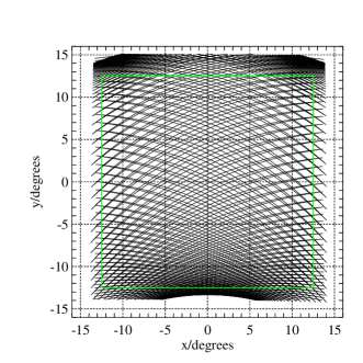
Figure 2: The path of the central focal-plane pixel for the semi-realistic scan. The scan is based on a 24-h constant-elevation scan from Dome-C. The green (solid) square shows the region used in the analysis and over which the fields were taken to be periodic.

We use a combination of the analytic results in Section 5 and simulations to find the mean change in the power spectrum and its variance and hence find tolerance limits for each systematic parameter considered in Sections 3 and 4.2. We vary each parameter individually and so do not account for cross-terms between parameters. The results are summerized in Table 1 for our toy-model of odd-parity cross-polar optics. The corresponding power spectrum perturbations for the semi-realistic scan are shown in Figs. 3–5. For all parameters apart from $e_{s}$ and ${\mn@boldsymbol{p}}$, the power spectrum perturbations and tolerance limits were evaluated using the semi-analytic and both of the simulation methods outlined in Section 5, with the different methods showing good agreement. Figure 3 compares the power spectrum perturbations obtained using the analytic and interpolation simulation method for a selection of the parameters for the semi-realistic scan. The good agreement of these methods validates the low-order expansions used in our analytic work, and is representative of all the parameters considered. Power spectrum perturbations for the remaining parameters for the semi-realistic scan, calculated with the semi-analytic method, are shown in Fig. 4. For $e_{s}$ and ${\mn@boldsymbol{p}}$, the assumption that the parameters are small breaks down below the tolerance limit, and so we rely on the interpolation simulation method to obtain limits and power spectrum perturbations (shown in Fig. 5) for these parameters.

Table 1: Tolerance limits for systematic errors. Three different scan strategies are considered: a raster scan, an ideal scan, and a semi-realistic scan (see text for details). The cross-polar results are for our odd-parity toy-model.

Parameter	Raster	Ideal	Semi-realistic
$a$	$5.10\times 10^{-3}$	$5.10\times 10^{-3}$	$5.10\times 10^{-3}$
$\omega$	$4.30\times 10^{-3}$	$4.30\times 10^{-3}$	$4.30\times 10^{-3}$
$f_{1}$	$1.27\times 10^{-2}$	$\infty$	$5.33\times 10^{-2}$
$f_{2}$	$1.18\times 10^{-2}$	$\infty$	$5.23\times 10^{-2}$
$\gamma_{1}$	$1.61\times 10^{-4}$	$\infty$	$2.22\times 10^{-4}$
$\gamma_{2}$	$1.51\times 10^{-4}$	$\infty$	$2.10\times 10^{-4}$
$e_{s}$	$5.6\times 10^{-1}$	$5.5\times 10^{-1}$	$3.1\times 10^{-1}$
$q$	$1.20\times 10^{-2}$	$7.26\times 10^{-2}$	$5.39\times 10^{-2}$
$p_{x}$	$-$	$7.3\times 10^{-1}$	$1.0\times 10^{-1}$
$p_{y}$	$-$	$7.3\times 10^{-1}$	$6.0\times 10^{-1}$
$b_{d,x}$	$2.05\times 10^{-3}$	$1.15\times 10^{-1}$	$2.82\times 10^{-3}$
$b_{d,y}$	$2.05\times 10^{-3}$	$1.15\times 10^{-1}$	$2.84\times 10^{-3}$
$\nu_{a,R}$	$2.55\times 10^{-2}$	$7.26\times 10^{-2}$	$2.77\times 10^{-2}$
$\nu_{d,R}$	$1.02\times 10^{-3}$	$\infty$	$1.41\times 10^{-3}$
$\nu_{a,I}$	$7.26\times 10^{-2}$	$7.26\times 10^{-2}$	$7.25\times 10^{-2}$
$\nu_{d,I}$	$1.12\times 10^{-1}$	$\infty$	$2.31\times 10^{-1}$

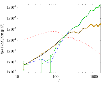
Figure 3: Power spectrum perturbations for $b_{d,x}$ and $q$ for the semi-realistic scan calculated with our semi-analytical method (black, solid and blue, dashed respectively) and with 1000 simulations (orange, dash-dotted and green, long-dashed respectively). The error bars are estimates of the theoretical error in the mean of the 1000 simulations due to their finite number. Note the good agreement between the two methods. For the simulations the scan is interpolated at intervals of $3.6^{\circ}$, and it is this interpolation that leads to the small deviations between the two methods evident for $q$ at $l<200$. The $B$-mode power spectrum from gravitational waves with $r=0.01$ is shown in red (dotted) for comparison.

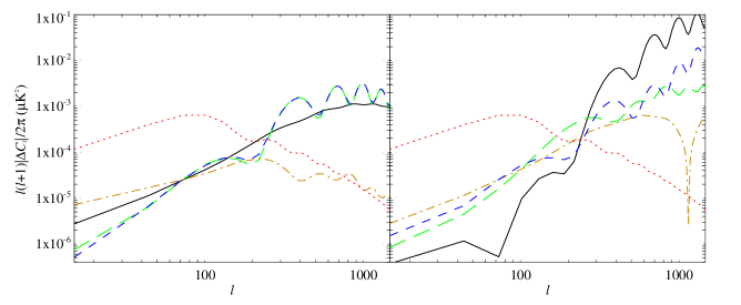
Figure 4: Power spectra perturbations for the semi-realistic scan corresponding to the tolerance limits for: (left) $a$ (black, solid), $\omega$ (green, long-dashed), $\gamma$ (orange, dash-dotted) and $f$ (blue, dashed); and (right) $\nu_{a,R}$ (black, solid), $\nu_{d,R}$ (green, long-dashed), $\nu_{a,I}$ (orange, dash-dotted) and $\nu_{d,I}$ (blue, dashed). The $B$-mode power spectrum from gravitational waves with $r=0.01$ is shown in red (dotted) for comparison.

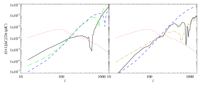
Figure 5: Simulated power spectra perturbations for $e_{s}$ (left) and $p_{x}$ (right) for $1000$ simulations for a raster (green, long-dashed), ideal (blue, dashed) and semi-realistic (black, solid) scan. On the left, the perturbation for $p_{y}$ for a semi-realistic scan is also shown (orange, dash-dotted). The $B$-mode power spectrum from gravitational waves with $r=0.01$ is shown in red (dotted) for comparison.

In every case, the limiting criterion is the bias in $r$ which is always at least an order of magnitude greater than the increase in the random error, $\sigma_{r}$. This is a result of the lensing induced $B$-modes dominating the variance in the power spectrum on large scales. To see this it is useful to write $\alpha$ and $\beta$ as

$$\alpha\approx\left.\frac{r^{2}}{2}\sum_{b}\left(\frac{\partial_{r}C^{B}_{b}}{\sigma_{b}}\right)^{2}\frac{\langle\Delta\hat{C}^{B}_{b,\mathrm{obs}}\rangle}{C_{b,\mathrm{prim}}^{B}}\right|_{r=0.01}$$ (128)

$$\beta\approx\left.\frac{r^{2}}{8}\sum_{b}\left(\frac{\partial_{r}C^{B}_{b}}{\sigma_{b}}\right)^{2}\frac{\Delta\mathrm{var}(\hat{C}^{B}_{b,\mathrm{obs}})}{\sigma_{b}^{2}}\right|_{r=0.01},$$ (129)

where we have made use of equations (123)–(127) and the fact that $\sigma_{r}|_{r=0.01}\approx r/2$ by design. $C_{b,\mathrm{prim}}^{B}$ is the primordial $B$-mode power spectrum due to gravitational waves. Written like this we see that $\alpha$ depends on the ratio of the bias in the power spectrum to the primordial spectrum, whilst $\beta$ depends on the ratio of the change in the variance to the ideal variance in a similar manner. As a result, the large contribution of gravitational lensing to the $B$-modes suppresses $\beta$ relative to $\alpha$. Taking an $\omega$ error as an example, from the results of Section 5 we find ${\langle\Delta\hat{C}^{B}_{b,\mathrm{obs}}\rangle}/{C_{b,\mathrm{prim}}^{B}}=4\omega^{2}C^{E}_{b}/C^{B}_{b,\mathrm{prim}}$ whilst ${\Delta\mathrm{var}(\hat{C}^{B}_{b,\mathrm{obs}})}/{\sigma_{b}^{2}}=8\omega^{2}C^{E}_{b}/C^{B}_{b}$ to leading order in $\omega$. As $C^{B}_{b}>C_{b,\mathrm{prim}}^{B}$ at all scales of interest, $\alpha>\beta$. Note that this assumes we cannot access the reionization information: for an experiment with sufficient sky coverage, the reionization peak, which is expected to dominate the power spectrum at very large scales, will be resolved and so the increase in random error will be more significant.

As expected, the limits for $a$ and $\omega$ are independent of the scan strategy, as they simply rescale the $Q\pm iU$ spin states and the errors they introduce transform like a true polarization. The limit for $a$ is more strict than might naïvely be expected, as the error not only amplifies the primordial spectrum, but also leads to imperfect subtraction of the lensing contribution. For the raster scan, there are no limits for an average co-polar pointing error, ${\mn@boldsymbol{p}}$, as a global displacement has no effect on the power spectrum. For the ideal scan, $\gamma_{1}$, $\gamma_{2}$, $f_{1}$, $f_{2}$, $\nu_{d,R}$ and $\nu_{d,I}$ are not constrained since the errors they produce disappear when averaged over all orientations.

Comparing the semi-realistic scan to the raster scan, many of the tolerances are relaxed as a result of the cross-linking, but the improvement is relatively modest. In the case of the tightest tolerances, those for $\gamma_{1}$ and $\gamma_{2}$ which leak temperature into linear polarization, the limits are only relaxed by around $40$ per cent, which suggests that our ability to control these errors with beam rotation is limited. Although an ideal scan removes these errors completely, a scan that covers $90$ per cent of basis orientations only relaxes the limits by a factor of $10$. That is, the cross-linking needs to be almost complete before we see significant changes in the tolerances, and so demanding such improvement would put considerable constraints on the scan strategy. Such constraints are unlikely to be compatible with other constraints such as the desire to use constant-elevation scans to avoid gradients in the average atmospheric signal. Having the ability to rotate the instrument directly about its boresight, rather than relying on rotation induced by scanning (and sky rotation), will likely prove very useful for efficient suppression of some systematics in future ground-based surveys.

The semi-realistic scan introduces a further new feature over the raster and ideal scan: not every pixel is seen at the same angles $\psi$, so there is differential beam rotation across the field. This gives rise to new effects, such as transformation of $E$-modes into observed $B$-modes even for an experiment with no cross-polarization, and identical coupling to the sky and propagation through the receiver for the two polarizations. Consider an otherwise ideal instrument with equal elliptical co-polar beams for the $A$ and $B$ polarizations. If the range of $\psi$ were the same in every pixel, the observed $Q$ and $U$ maps would simply be the true maps convolved with some effective beam; this does not produce any transformation of $E$-modes into $B$. Similar comments apply to a common pointing error, ${\mn@boldsymbol{p}}$, with otherwise ideal optics. The effect of differential beam rotation in the errors from the average ellipticity, $e_{s}$, and pointing parameters can be seen in Fig. 5, which shows the power spectrum perturbations for these parameters for all three scan strategies. For both parameters, transformation of $E$-modes to $B$-modes leads to an increase in the bias at low $l$. However, this does not lead to a significant tightening of the tolerances. This is partly fortuitous, as the $E$-to-$B$ errors from differential beam rotation contribute with opposite sign to the $B$-to-$B$ errors that the parameters contribute for an ideal scan. The $E$-to-$B$ effect may be more significant for a more realistic scan, perhaps requiring multiple elevation scans to cover the survey region. (Interestingly, demanding better cross-linking to control temperature leakage, and suppress low-frequency noise, is likely to result in a more complex scan strategy with increased differential rotation.) As an extreme example, we can examine the effects of a scan in which the basis orientation for each sky pixel is selected at random, as we might expect this to maximize differential rotation. With such a scan, the limits become $0.024$ for $e_{s}$ and $0.058$ for $|{\mn@boldsymbol{p}}|$ which are still not particularly tight. These results suggests that, provided we avoid pathologically-constructed scans, transformation of $E$-modes to $B$-modes from differential rotation is unlikely to be significant. However, transformation of $E$-to-$B$ through cross-polarization always warrants careful control.

7.2 Real Beams

So far we have considered the impact of specific beam non-idealities that can be simply parametrized. However, there may be significant effects from beam characteristics that are unexpected, or not easily parametrized and are not present in our simple beam models. Therefore, in this section we will extend our scope to examine the effects of real, or simulated, beam patterns. For simplicity, we will only consider raster and ideal scans. From simulations of the far-field patterns, ${\mn@boldsymbol{E}}_{A}$ and ${\mn@boldsymbol{E}}_{B}$, we can form the beam Müller fields using equation (72). Then, from equation (103), we can calculate the bias in the recovered power spectrum, and from that the bias in $r$. We simulated beam patterns for a realistic optical setup with a physical-optics code. (Specifically, the simulations were done in the context of the Clover experiment.) Beams were simulated for three different focal plane positions: the central pixel and two pixels at the edge of the array, displaced from the centre along the optical axes. These pixels are expected to be representative of the entire array. A re-calibration of the beam centres and axes was performed to remove simulation artifacts. The power profiles in co- and cross-polarization for the two polarization states of the central pixel and one edge pixel are shown in Fig. 6 (the remaining edge pixel having similar features to the one shown). One new feature, not considered in our previous analysis, that is immediately evident from these profiles is the subsidiary maxima present in the co-polar beams. These sidelobe features would not be easy to parametrize, particularly for the pixels at the focal plane edge where the effect breaks the azimuthal symmetry of the profiles. When evaluating systematic effects, we assumed the data analysis would be performed with Gaussian co-polar beams, with relative powers and beam sizes matched to the simulated beams. We analysed each pixel separately, but scaled the noise down to a value appropriate for a 500-element array. This is equivalent to assuming that every pixel in the focal plane has the same imperfect optical response. We performed our analysis with an ideal receiver.

Figure 6: Simulated (power) beam patterns for a realistic optical setup. Panels (a)–(d) show $|E_{A\,\mathrm{co}}|^{2}$, $|E_{B\,\mathrm{co}}|^{2}$, $|E_{A\,\mathrm{cross}}|^{2}$ and $|E_{B\,\mathrm{cross}}|^{2}$ for a central, on-axis pixel, and panels (e)–(h) show the same for a pixel at the edge of the focal plane array. The average total power in the cross-polar beams, relative to the corisponding co-polar beams is $2.2\times 10^{-7}$ for the central pixel, and $2.3\times 10^{-6}$ for the shifted pixel. The contours are at $-3$ dB intervals, down to $-57$ dB for the co-polar beams, and $-30$ dB for the cross-polar beams.

For the central focal plane pixel $\alpha$ is around $2$ per cent, irrespective of the scan strategy. Of the pixels considered, this is the worst case (with $\alpha$ well below the per cent level for the remaining pixels) and is well within the tolerance limits we have previously suggested. Furthermore, this bias is mainly a result of our assumption of simple Gaussian beams in the analysis, and could be reduced by a more sophisticated treatment of the average, symmetric co-polar beam profiles. Fig. 7 shows the perturbations to the power spectrum for a raster scan. The perturbations are largely independent of the scan strategy, and due almost entirely to the true $B$-modes: the contribution from total intensity and $E$-modes is always below $10^{-6}~{}\mu\mathrm{K}^{2}$. These results were confirmed by direct convolution of simulated Stokes maps with the Müller beams. These simulations also confirmed that the increase in the random error in $r$ is sub-dominant to the bias, as expected from Section 7.1.

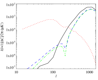
Figure 7: Perturbations to the $B$-mode power spectrum for the central focal plane pixel (black, solid) and the edge pixels (blue, dotted and green, dash-dotted) for a raster scan. (For the edge pixels, the perturbations are negative below the kink at $l\sim 200$.) The $B$-mode power spectrum from gravitational waves with $r=0.01$ is shown in red (dotted) for comparison.

8 Discussion

We have presented a framework to describe, in a general manner, the scientific impact of instrumental systematic errors in CMB polarimetry experiments surveying small sky areas. A major focus was the behaviour of systematic errors under instrument rotation. We introduced spin-weighted Müller matrices to describe the propagation of the Stokes parameters through the receiver to simplify the transformation properties of the systematic effects under rotations. The optical coupling of the receiver to the incoming radiation field is described by Müller matrix-valued fields. We gave expressions for these in terms of the vector-valued field pattern of the antenna, and introduced a convenient decomposition of the matrix fields into components that transform irreducibly under rotations. The decomposition is useful for analytical work and also provides an efficient means of simulating the effect in Stokes maps of systematic effects for an arbitrary scan strategy.

We compared two popular receiver architectures for CMB polarimetry and showed that modulating the polarization with a half-wave plate has the advantage over a pseudo-correlation receiver of producing no instrumental polarization for ideal optics. It should be noted that, in the presence of realistic optics, the half-wave-plate receiver will contribute to instrumental polarization, but at a higher order in the parameters describing systematics than the pseudo-correlation receiver. This result holds for a waveplate in waveguide – further analysis is required for a quasi-optical approach where the waveplate is before the beam-defining element (and typically is at the beam waist). We also analysed simple parametrized models for imperfect co- and cross-polar beams and presented the irreducible components of their Müller fields.

We presented an efficient, semi-analytic method for calculating the bias in the power spectra from time-invariant instrument systematics described by an arbitrary Müller response, and for a general scan strategy. This should prove useful for setting tolerance limits during the design phase of an experiment. However, since the analysis is entirely in the map domain, detailed simulations will still be required for data analysis to account properly for the interaction of non-trivial map-making with systematic effects. We also analysed the extreme cases of scans with no and complete beam rotation and obtained simple results for the biases induced in the $B$-mode power spectrum, and the increase in the random error in the power spectrum. Several important effects are missed by these extreme scans, such as the generation of $B$-modes from $E$-modes, even in the absence of cross-polarization, by differential beam rotation across the observed field. It is often important to propagate the effects of systematic errors through to cosmological parameters to assess properly their effect on the scientific returns. We did this for the tensor-to-scalar ratio for a survey representative of that from next-generation ground-based instruments, and set tolerance limits for simple parametrized forms of the receiver and optical systematics. The formalism can also be applied to non-parametric, simulated or measured beam models and we illustrated this with the results of physical optics simulations.

Although instrument rotation is potentially a powerful way to mitigate against stable instrumental systematic effects, we showed that for a typical scan that can be obtained reasonably from the ground, the limited range of angles at which a pixel is revisited limits the extent to which systematics can be controlled. For the semi-realistic scan considered here we found that tolerance limits on systematics could be relaxed by between 40 and 400 per cent over those for a simple raster scan. For all cases considered here, the tolerance limits for a realistic scan are never significantly stricter than for a raster scan. The distribution of scan angles $\psi$ can be improved considerably for constant-elevation scans by including $z$-axis rotation, rather than relying on sky rotation. This may prove to be an important element of future campaigns to detect primary $B$-mode polarization in the CMB.

As previously noted, this paper does not directly consider some important time-invariant systematic errors. For example, as we have restricted our analysis to quasi-monochromatic systems, errors such as bandpass mismatch, and other variations in instrumental response with frequency have been ignored. However, the methods and analysis introduced in this paper can be straightforwardly extended to accommodate such errors by splitting the bandwidth up into a number of sub-bands in which the instrumental response can reasonably be modelled as constant, and allowing systematics to vary between the sub-bands. Each sub-band can be treated independently and the Müller matrix used to describe the whole instrument simply becomes an appropriately weighted sum over the matrices for each band, and the analysis can proceed unhindered.

9 Acknowledgments

D.O. acknowledges a PPARC studentship. A.C. is supported by a Royal Society University Research Fellowship. B.R.J. acknowledges support from a PPARC Postdoctoral Fellowship and an NSF IRFP Postdoctoral Fellowship. We thank members of the Clover collaboration for helpful discussions, particularly Paul Grimes who also provided an early version of the physical-optics simulations discussed in Section 7.2.

Appendix A Complex beam MÜller fields

We can extract the complex beam Müller fields from the real components in equation (72). Those fields for which the second index has non-zero spin are best expressed in terms of the spin-$\pm 1$ components of $\mn@boldsymbol{E}_{A}$ and $\mn@boldsymbol{E}_{B}$:

$${}_{\pm 1}E_{A} \equiv \mn@boldsymbol{E}_{A}\cdot(\hat{{\mn@boldsymbol{x}}}\pm i\hat{{\mn@boldsymbol{y}}})=E_{A\,\mathrm{co}}\mp iE_{A\,\mathrm{cross}}$$

$${}_{\pm 1}E_{B} \equiv \mn@boldsymbol{E}_{B}\cdot(\hat{{\mn@boldsymbol{x}}}\pm i\hat{{\mn@boldsymbol{y}}})=-E_{B\,\mathrm{cross}}\mp iE_{B\,\mathrm{co}},$$ (130)

whereas those with spin-$0$ component can be expressed directly in terms of scalar products of $\mn@boldsymbol{E}_{A}$, $\mn@boldsymbol{E}_{B}$ and their duals

$${}^{\star}\!\mn@boldsymbol{E}_{A}\equiv-\left(\begin{array}[]{c}E_{A\,\mathrm{cross}}\\ E_{A\,\mathrm{co}}\end{array}\right),\quad{}^{\star}\!\mn@boldsymbol{E}_{B}\equiv\left(\begin{array}[]{c}-E_{B\,\mathrm{co}}\\ E_{B\,\mathrm{cross}}\end{array}\right),\quad$$ (131)

which are obtained by a right-handed rotation through 90° about the radiation propagation direction. The independent components of the complex Müller  fields are

$$M_{TT} = {\textstyle{\frac{1}{2}}}(|{\mn@boldsymbol{E}}_{A}|^{2}+|{\mn@boldsymbol{E}}_{B}|^{2})$$

$$M_{TP} = {\textstyle{\frac{1}{4}}}({}_{1}E_{A}{}_{-1}E_{A}^{*}+{}_{1}E_{B}{}_{-1}E_{B}^{*})$$

$$M_{TV} = {\textstyle{\frac{1}{2}}}i({}^{\star}\!\mn@boldsymbol{E}_{A}\cdot\mn@boldsymbol{E}_{A}^{*}+{}^{\star}\!\mn@boldsymbol{E}_{B}\cdot\mn@boldsymbol{E}_{B}^{*})$$

$$M_{PT} = {\textstyle{\frac{1}{2}}}(\mn@boldsymbol{E}_{A}+i\mn@boldsymbol{E}_{B})\cdot(\mn@boldsymbol{E}_{A}-i\mn@boldsymbol{E}_{B})^{*}$$

$$M_{PP} = {\textstyle{\frac{1}{4}}}({}_{1}E_{A}+i{}_{1}E_{B})({}_{-1}E_{A}-i{}_{-1}E_{B})^{*}$$

$$M_{PP^{*}} = {\textstyle{\frac{1}{4}}}({}_{-1}E_{A}+i{}_{-1}E_{B})({}_{1}E_{A}-i{}_{1}E_{B})^{*}$$

$$M_{PV} = {\textstyle{\frac{1}{2}}}i({}^{\star}\!\mn@boldsymbol{E}_{A}+i{}^{\star}\!\mn@boldsymbol{E}_{B})\cdot(\mn@boldsymbol{E}_{A}-i\mn@boldsymbol{E}_{B})^{*}$$

$$M_{VT} = {\textstyle{\frac{1}{2}}}i(-\mn@boldsymbol{E}_{A}\cdot\mn@boldsymbol{E}_{B}^{*}+\mn@boldsymbol{E}_{B}\cdot\mn@boldsymbol{E}_{A}^{*})$$

$$M_{VP} = -{\textstyle{\frac{1}{4}}}i({}_{1}E_{A}{}_{-1}E_{B}^{*}-{}_{1}E_{B}{}_{-1}E_{A}^{*})$$

$$M_{VV} = {\textstyle{\frac{1}{2}}}({}^{\star}\!\mn@boldsymbol{E}_{A}\cdot\mn@boldsymbol{E}_{B}^{*}-{}^{\star}\!\mn@boldsymbol{E}_{B}\cdot\mn@boldsymbol{E}_{A}^{*}).$$ (132)

Expressed this way, the transformation properties under a rotation of the coordinate basis on the sky are manifest.

Appendix B Beam expansion

The expansion of the beam in equation (75) can be written as

$${\textbf{{M}}}({\mn@boldsymbol{x}}) = \frac{e^{-{\mn@boldsymbol{x}}^{2}/2\sigma^{2}}}{2\pi\sigma^{2}}\sum_{mn}\Bigl{[}{\textbf{{M}}}_{mn}(-1)^{n}2^{m}m!\left(\frac{x-iy}{\sigma}\right)^{n-m}$$ (133)

$$\mbox{}\hskip 43.36464pt\times L_{m}^{n-m}({\mn@boldsymbol{x}}^{2}/2\sigma^{2})\bigr{]},$$

where $L_{n}^{\alpha}$ is the Laguerre polynomial (Gradshteyn & Ryzhik, 2000), familiar from the radial wavefunctions of the Hydrogen atom. Each term in the sum is a Gaussian multiplying a polynomial in $x$ and $y$. Equation (133) can be inverted using the orthogonality of the Laguerre polynomials:

$${\textbf{{M}}}_{mn}=\frac{(-1)^{n}}{2^{n}n!}\int{\mathrm{d}}^{2}{\mn@boldsymbol{x}}\,{\textbf{{M}}}\left(\frac{x+iy}{\sigma}\right)^{n-m}L_{m}^{n-m}({\mn@boldsymbol{x}}^{2}/2\sigma^{2}).$$ (134)

Note that, for $m>n$ with $m$ and $n\geq 0$, $L_{m}^{n-m}(x)=O(x^{m-n})$ so that the integrand in this equation is always regular at the origin.

In Section 4.2 we introduced a simple parametrization for offset, elliptical co-polar beams and two toy-model examples of cross-polar beams. Here we give the ${\textbf{{M}}}_{mn}$ matrices for these parametrized beams to first order in the parameters. Generally, if the maximum order of the polynomials appearing in equation (133) is $l$, then there are terms present with $m$ and $n$ taking all integer values $\geq 0$ such that $m+n\leq l$. For a first-order expansion of the beam models of Section 4.2, $l=2$. Adopting a matrix notation for the indices $m$ and $n$, we find for the case of Gaussian cross-polar beams that

$$[{\textbf{{M}}}_{mn}]_{TT} = \left(\begin{array}[]{ccc}1&-({}_{1}p/2)&e_{s}/2\\ -({}_{-1}p/2)&0&0\\ e_{s}/2&0&0\end{array}\right)$$ (138)

$${[{\textbf{{M}}}_{mn}]}_{TP} = \left(\begin{array}[]{ccc}-i\nu_{d,R}&-({}_{1}b_{d}/4)&q/4\\ -({}_{-1}b_{d}/4)&0&0\\ q/4&0&0\end{array}\right)$$ (142)

$${[{\textbf{{M}}}_{mn}]}_{PT} = \left(\begin{array}[]{ccc}2i\nu_{d,R}&-({}_{1}b_{d}/2)&q/2\\ -({}_{-1}b_{d}/2)&0&0\\ q/2&0&0\end{array}\right)$$ (146)

$${[{\textbf{{M}}}_{mn}]}_{PP} = \left(\begin{array}[]{ccc}1-2i\nu_{a,R}&-({}_{1}p/2)&e_{s}/2\\ -({}_{-1}p/2)&0&0\\ e_{s}/2&0&0\end{array}\right)$$ (150)

$${[{\textbf{{M}}}_{mn}]}_{VV} = \left(\begin{array}[]{ccc}1&-({}_{1}p/2)&e_{s}/2\\ -({}_{-1}p/2)&0&0\\ e_{s}/2&0&0\end{array}\right);$$ (154)

the remaining independent, non-zero elements are $[{\textbf{{M}}}_{00}]_{TV}=2\nu_{a,R}=[{\textbf{{M}}}_{00}]_{VT}$, $[{\textbf{{M}}}_{00}]_{PV}=2\nu_{d,I}=-2[{\textbf{{M}}}_{00}]_{VP}$ and $[{\textbf{{M}}}_{00}]_{VT}=2\nu_{a,I}$. Here, for example, ${}_{\pm 1}p\equiv{\mn@boldsymbol{p}}\cdot(\hat{{\mn@boldsymbol{x}}}\pm\hat{{\mn@boldsymbol{y}}})$ are the spin-$\pm 1$ components of ${\mn@boldsymbol{p}}$. For the power spectrum analysis in Section 5 we need some elements of $M_{PP}$ and $M_{PP^{*}}$ to second-order in the systematics as these appear multiplying the zero-order Müller matrix. The relevant second-order, non-zero terms are

$${[{\textbf{{M}}}_{00}]}_{PP} = -{\mn@boldsymbol{b}}_{d}^{2}/4-q^{2}-(\nu_{a,R}^{2}+\nu_{a,I}^{2})$$

$${[{\textbf{{M}}}_{11}]}_{PP} = {\mn@boldsymbol{p}}^{2}/4+{\mn@boldsymbol{b}}_{d}^{2}/8+e_{s}^{2}/2-q^{2}/2$$

$${[{\textbf{{M}}}_{22}]}_{PP} = e_{s}^{2}/4+q^{2}/8$$

$${[{\textbf{{M}}}_{04}]}_{PP^{\ast}} = q^{2}/16={[{\textbf{{M}}}_{40}]}_{PP^{\ast}}.$$ (155)

For the cross-polar beams with a single line of symmetry, $[{\textbf{{M}}}_{mn}]_{TT}$ and $[{\textbf{{M}}}_{mn}]_{VV}$ are unchanged from equation (154) but

$${[{\textbf{{M}}}_{mn}]}_{TP} = -\frac{1}{4}\left(\begin{array}[]{ccc}0&{}_{1}b_{d}+2\nu_{d,R}&-q\\ {}_{-1}b_{d}-2\nu_{d,R}&0&0\\ -q&0&0\end{array}\right)$$ (159)

$${[{\textbf{{M}}}_{mn}]}_{PT} = -\frac{1}{2}\left(\begin{array}[]{ccc}0&{}_{1}b_{d}-2\nu_{d,R}&-q\\ {}_{-1}b_{d}+2\nu_{d,R}&0&0\\ -q&0&0\end{array}\right)$$ (163)

$${[{\textbf{{M}}}_{mn}]}_{PP} = -\frac{1}{2}\left(\begin{array}[]{ccc}-2&{}_{1}p+2\nu_{a,R}&-e_{s}\\ {}_{-1}p-2\nu_{a,R}&0&0\\ -e_{s}&0&0\end{array}\right).$$ (167)

The remaining independent non-zero elements are $[{\textbf{{M}}}_{01}]_{TV}=-i\nu_{a,I}=-[{\textbf{{M}}}_{10}]_{TV}$, $[{\textbf{{M}}}_{01}]_{PV}=-i\nu_{d,I}=-[{\textbf{{M}}}_{10}]_{PV}$, $[{\textbf{{M}}}_{01}]_{VT}=-i\nu_{a,I}=-[{\textbf{{M}}}_{10}]_{VT}$ and $[{\textbf{{M}}}_{01}]_{VP}=i\nu_{d,I}/2=-[{\textbf{{M}}}_{10}]_{VP}$. The second-order terms required for a consistent power spectrum calculation are, in this case,

$${[{\textbf{{M}}}_{00}]}_{PP} = -{\mn@boldsymbol{b}}_{d}^{2}/4-q^{2}-(\nu_{a,R}^{2}+\nu_{a,I}^{2})-ip_{y}\nu_{a,R}$$

$${[{\textbf{{M}}}_{11}]}_{PP} = {\mn@boldsymbol{p}}^{2}/4+{\mn@boldsymbol{b}}_{d}^{2}/8+e_{s}^{2}/2-q^{2}/2$$

$$\mbox{}-(\nu_{a,R}^{2}+\nu_{a,I}^{2})/2-ip_{y}\nu_{a,R}/2$$

$${[{\textbf{{M}}}_{22}]}_{PP} = e_{s}^{2}/4+q^{2}/8$$

$${[{\textbf{{M}}}_{04}]}_{PP^{\ast}} = q^{2}/16={[{\textbf{{M}}}_{40}]}_{PP^{\ast}}.$$ (169)

References

- Barkats et al. (2005) Barkats D. et al., 2005, ApJ, 619, L127
- Barkats et al. (2005) Barkats D. et al., 2005, ApJS, 159, 1
- Bucher et al. (2001) Bucher M., Moodley K., Turok N., 2001, Phys. Rev. Lett., 87, 191301
- Bunn (2006) Bunn E. F., 2006, preprint (astro-ph/0607312)
- Carretti et al. (2004) Carretti E., Cortiglioni S., Sbarra C., Tascone R., 2004, A&A, 420, 437
- Efstathiou & Bond (1999) Efstathiou G., Bond J. R., 1999, MNRAS, 304, 75
- Feng et al. (2006) Feng B., Li M., Xia J.-Q., Chen X., Zhang X., 2006, Phys. Rev. Lett., 96, 221302
- Gradshteyn & Ryzhik (2000) Gradshteyn, I. S., Ryzhik, I. M., 2000, Table of integrals, series and products, 6th edn. Academic Press, New York
- Hu et al. (2003) Hu W., Hedman M. M., Zaldarriaga M., 2003, Phys. Rev. D, 67, 043004
- Hu & Okamoto (2002) Hu W., Okamoto T., 2002, ApJ, 574, 566
- Jarosik et al. (2006) Jarosik N. et al., 2006, preprint (astro-ph/0603452)
- Johnson et al. (2007) Johnson B. R. et al., 2007, ApJ, in press (astro-ph/0611394)
- Jones et al. (2006) Jones W. C. et al., 2006, preprint (astro-ph/0606606)
- Kamionkowski et al. (1997) Kamionkowski M., Kosowsky A., Stebbins A., 1997, Phys. Rev. D, 55, 7368
- Kovac et al. (2002) Kovac J. M., Leitch E. M., Pryke C., Carlstrom J. E., Halverson N. W., Holzapfel W. L., 2002, Nat, 420, 772
- Lewis & Challinor (2006) Lewis A., Challinor A., 2006, Phys. Reports, 429, 1
- Lewis et al. (2002) Lewis A., Challinor A., Turok N., 2002, Phys. Rev. D, 65, 023505
- Lue et al. (1999) Lue A., Wang L., Kamionkowski M., 1999, Phys. Rev. Lett., 83, 1506
- Masi et al. (2006) Masi S. et al., 2006, A&A, 458, 687
- Montroy et al. (2006) Montroy T. E. et al., 2006, ApJ, 647, 813
- Page et al. (2006) Page L. et al., 2006, preprint (astro-ph/0603450)
- Readhead et al. (2004) Readhead A. C. S. et al., 2004, Sci, 306, 836
- Scannapieco & Ferreira (1997) Scannapieco E. S., Ferreira P. G., 1997, Phys. Rev. D, 56, 7493
- Smith et al. (2004) Smith K. M., Hu W., Kaplinghat M., 2004, Phys. Rev. D, 70, 043002
- Smith et al. (2006) Smith S., Challinor A., Rocha G., 2006, Phys. Rev. D, 73, 023517
- Spergel et al. (2006) Spergel D. N. et al., 2006, preprint (astro-ph/0603449)
- Wu et al. (2007) Wu J. H. P. et al., 2007, ApJ, in press, (astro-ph/0611392)
- Zaldarriaga (1997) Zaldarriaga M., 1997, Phys. Rev. D, 55, 1822
- Zaldarriaga & Seljak (1997) Zaldarriaga M., Seljak U., 1997, Phys. Rev. D, 55, 1830
- Zaldarriaga & Seljak (1998) Zaldarriaga M., Seljak U., 1998, Phys. Rev. D, 58, 023003
- Zaldarriaga et al. (1997) Zaldarriaga M., Spergel D. N., Seljak U., 1997, ApJ, 488, 1