Oxygen, Sodium, Magnesium and Aluminium as tracers of the Galactic Bulge Formation

Abstract

Aims. This paper investigates the peculiar behaviour of the light even (alpha-elements) and odd atomic number elements in red giants in the galactic bulge, both in terms of the chemical evolution of the bulge, and in terms of possible deep-mixing mechanisms in these evolved stars.

Methods. Abundances of the four light elements O, Na, Mg and Al are measured in 13 core He-burning giants stars (red clump stars) and 40 red giant branch stars in four 25$\arcmin$ fields spanning the bulge from $-3$ to $-12$ of galactic latitude. Special care was taken in the abundance analysis, performing a differential analysis with respect to the metal-rich solar-neighbourhood giant $\mu$Leo which resembles best our bulge sample stars. This approach minimizes systematic effects which can arise in the analysis of cool metal-rich stars due to continuum definition issues and blending by molecular lines (CN) and cancels out possible model atmosphere deficiencies.

Results. We show that the resulting abundance patterns point towards a chemical enrichment dominated by massive stars at all metallicities. Oxygen, magnesium and aluminium ratios with respect to iron are overabundant with respect to both galactic disks (thin and thick) for [Fe/H]$>-0.5$. A formation timescale for the galactic bulge shorter than for both the thin and thick disks is therefore inferred.

To isolate the massive-star contribution to the abundances of O, Mg, Al and Na, we use Mg as a proxy for metallicity (instead of Fe), and further show that: (i) the bulge stars [O/Mg] ratio follows and extend to higher metallicities the decreasing trend of [O/Mg] found in the galactic disks. This is a challenge for predictions of O and Mg yields in massive stars which so far predicted no metallicity dependence in this ratio. (ii) the [Na/Mg] ratio trend with increasing [Mg/H] is found to increase in three distinct sequences in the thin disk, the thick disk and the bulge. The bulge trend is well represented by the predicted metallicity-dependent yields of massive stars, whereas the galactic disks have too high Na/Mg ratios at low metallicities, pointing to an additional source of Na from AGB stars. (iii) Contrary to the case of the [Na/Mg] ratio, there appears to be no systematic difference in the [Al/Mg] ratio between bulge and disk stars, and the theoretical yields by massive stars agree with the observed ratios, leaving no space for AGB contribution to Al.

1 Introduction

The bulge of the Milky Way galaxy harbours $\sim 10^{10}$$M_{\odot}$ of star, or, $\sim 20\%$ of the total stellar mass of our galaxy (Kent et al., 1991). From main sequence photometry the bulge stellar populations appear to be uniformly old, older than $\sim 10^{10}$ yrs (Ortolani et al., 1995; Zoccali et al., 2003), whereas they span a wide metallicity distribution, from [Fe/H] $\sim-1.5$ to $\sim+0.5$, and peaking around $\rm[Fe/H]=-0.2$ (McWilliam & Rich, 1994; Zoccali et al., 2003; Fulbright et al., 2006). It remains debatable weather our bulge is a classical bulge, formed in a merger-driven collapse, or a pseudo-bulge, formed by the secular dynamical evolution of the disk (Kormendy & Kennicutt, 2004).

A prompt formation, i.e., a short star formation phase resulting in a small age dispersion, may favor the classical-bulge option, but main-sequence photometry can hardly constrain the formation timescale to better than 2-3 Gyr. This leaves the pseudo-bulge option open provided the early disk ($\sim 10^{10}$ years ago) already contained $\sim 10^{10}$$M_{\odot}$ of stars and gas in its inner regions, and a bar instability promptly developed. Further constraints on the formation timescale can be inferred from the detailed chemical composition of bulge stars. As it is well known, $\alpha$-elements abundances relative to iron are sensitive to the star-formation timescale: as products of massive star evolution (exploding as Type II SNe) the $\alpha$-elements are almost instantaneously recycled in the interstellar medium (ISM), while a major fraction of iron is produced by Type Ia SNe which are characterized by a broad distribution of delay times between star formation and explosion (from few $10^{7}$ yrs to over $10^{10}$ yrs, e.g., Greggio, 2005).

The $\alpha$-elements abundances appear enhanced over iron in the bulge stars that have been analysed up to now iny Baade’s Window (McWilliam & Rich (1994): 12 K giants; McWilliam & Rich (2004): 9 stars; Fulbright et al. (2005): 20 stars; Rich & Origlia (2005): 10 M giants), as well as in a few stars per cluster in several bulge globular clusters ((Zoccali et al., 2004; Barbuy et al., 2006; Carretta et al., 2001; Origlia et al., 2005a, b)). The high $\alpha$-elements content of the bulge stellar population therefore hints at a short formation timescale. However, not all $\alpha$-elements share exactly the same nucleosynthetic history: whereas oxygen and magnesium are produced respectively during the helium- and carbon/neon-burning hydrostatic phases of massive stars, the heavier $\alpha$-elements (Si, Ca, Ti) are partly synthesized during the supernova explosion itself Woosley & Weaver (1995), and their yields are thus more uncertain. Moreover, a non-negligible fraction of silicon may also be produced by SNIa’s (e.g., Iwamoto et al., 1999). Hints for a different behaviour of various $\alpha$-elements the Galactic bulge have been already reported ((McWilliam & Rich, 1994, 2004; Zoccali et al., 2004))

Sodium and aluminium are odd-Z nuclei, that can also be produced in massive stars, chiefly during the C-burning phase. Their production is expected to be sensitive to the neutron excess Woosley & Weaver (1995), and through this, their yields are metallicity dependent, increasing with increasing metallicity. Besides, sodium can also be synthesized by $p$-captures through the Ne-Na cycle at the base of the convective envelope of AGB stars in the mass range $3{\mathrel{\mathchoice{\lower 2.9pt\vbox{\halign{$\m@th\displaystyle\hfil#\hfil$\cr<\crcr\sim\crcr}}}{\lower 2.9pt\vbox{\halign{$\m@th\textstyle\hfil#\hfil$\cr<\crcr\sim\crcr}}}{\lower 2.9pt\vbox{\halign{$\m@th\scriptstyle\hfil#\hfil$\cr<\crcr\sim\crcr}}}{\lower 2.9pt\vbox{\halign{$\m@th\scriptscriptstyle\hfil#\hfil$\cr<\crcr\sim\crcr}}}}}M{\mathrel{\mathchoice{\lower 2.9pt\vbox{\halign{$\m@th\displaystyle\hfil#\hfil$\cr<\crcr\sim\crcr}}}{\lower 2.9pt\vbox{\halign{$\m@th\textstyle\hfil#\hfil$\cr<\crcr\sim\crcr}}}{\lower 2.9pt\vbox{\halign{$\m@th\scriptstyle\hfil#\hfil$\cr<\crcr\sim\crcr}}}{\lower 2.9pt\vbox{\halign{$\m@th\scriptscriptstyle\hfil#\hfil$\cr<\crcr\sim\crcr}}}}}8\,$$M_{\odot}$ which are experiencing the envelope-burning process (e.g., Ventura & D’Antona, 2005). Similarly, aluminium can be produced in the same stars through the Mg-Al cycle, provided sufficiently high temperatures are reached.. Finally, the Ne-Na and Mg-Al cycles are also active in the deepest part of the hydrogen-burning shell of low-mass stars ascending the first in red giant branch (RGB), and their products may be brought to the surface if mixing processes are able to extend from the formal basis of the convective envelope all the way to almost the bottom of the burning shell (e.g., Weiss et al., 2000). In summary, there exists a multiplicity of potential sites were the O-Ne-Na and Mg-Al cycles can operate, i.e., in massive, intermediate-mass as well as low-mass stars. Therefore, the identification of the dominant site must be preliminary to an effective use of the relative abundances to set constraints on the timescale of bulge formation.

A widespread phenomenon among galactic globular clusters is the so-called O-Na and Mg-Al abundance anomalies. Whereas stars within a given cluster have a remarkably identical chemical abundances for most elements, high dispersions of these elements are observed that are underlined by anticorrelations of O with Na, and Mg with Al, and a correlation of Na and Al (see Gratton et al., 2004, for a review and references therein). To date, none of these anticorrelations have been observed in field stars of any metallicity and evolutionary stage, in particular among bulge stars. However, in the galactic bulge, aluminium appears to be slightly enhanced at all metallicities and especially so in the most metal-rich stars (McWilliam & Rich, 1994).

For many years, these abundances anomalies were observed only in bright RGB stars in globular clusters and were thought to be due to deep mixing bringing to the surface the products of self-made Na and Al through the O-Ne-Na and Mg-Al cycles (e.g., Weiss et al. 2000, and references therein). This idea was qualitatively consistent with the double-peaked distribution of carbon and nitrogen found in many clusters, also thought to be the result of internal mixing. The reason why this strong extra-mixing would occur only in globular clusters giants and not in their field counterparts was attributed to the difference in environment (that could lead to a different angular momentum history, hence in the extent of the mixed region due to either meridional circulation or shear mixing). This picture is now seriously challenged since similar anomalies, first in C and N Briley et al. (1991, 2004), and then in O, Na and Al Gratton et al. (2001) have been found also in stars on (or just evolved off) the main-sequence, whose maximum internal temperatures are not high enough to trigger either the O-Ne-Na or Mg-Al cycles. Current attempts at explaining the globular cluster abundance anomalies involve rather self-enrichment or pollution during the cluster formation or shortly thereafter, possibly in association with mixing along the RGB (Gratton et al., 2004; Charbonnel, 2005).

Using the same database as in the present paper, in Zoccali et al. (2006) the [O/Fe] vs. [Fe/H] ratios for bulge stars were presented, and compared to those of local thin disk and thick disk stars. In this paper we now examine the interrelations between O, Mg, Na and Al for 53 bulge giant stars, 40 on the RGB, and 13 in the red clump (core He burning stars) randomly drawn from the bulge metallicity distribution. This large sample allows us to see effects that were so far hidden in poor statistics, such as an O-Na anticorrelation and an Al-Na correlation, that we investigate in depth, examining the possible sources. In Section 2, the observations are summarized. Section 3 describes the method to derive stellar parameters, whereas the abundances of Na, Mg and Al are derived in Section 4. The results are presented in Section 5, mixing effects are examined in Section 6, and finally, nucleosynthesis yields and bulge abundance are compared in Section 7. A summary is given in Section 8.

2 Observations, data reduction

The observations were performed during several runs with the ESO-VLT-UT2 and the FLAMES (Fibre Large Array Multi-Element Spectrograph) instrument, and the final dataset combines data from the GTO program #071.B-0196 with others from the GO programs #071.B-0617 #073.B-0074. Details of the observations will be presented elsewhere (Zoccali et al., in preparation). In this paper, we analyse the stars observed with the red arm of the UVES spectrograph at a resolution R $\sim$ 47000 (Dekker et al., 2000) in the range 4800-6800 Å. The sample was drawn from four separate regions of the bulge and includes 13 red clump stars and 40 RGB stars $\sim$0.5 to 1 mag above the clump itself. Among them, 11 stars are located in a low reddening window at (l,b)=(0,-6), 26 stars in Baade’s Window at (l,b)=(1,-4, 5 stars in the Blanco field at (l,b)=(0,-12) and 13 stars in a field in the vicinity of the globular cluster NGC 6553 at (l,b)=(5,-3).

Fig. 1 shows, as an example, the location of our targets (RGB and Red Clump stars) on the I (V-I) colour-magnitude diagram of our Baade’s Window field (Paczynski et al., 1999, photometry from).

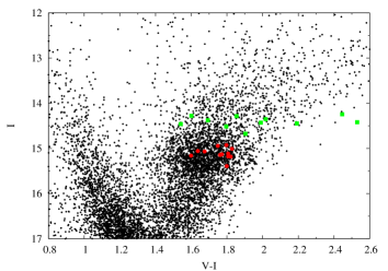
Figure 1: Colour magnitude diagram of our field in Baade’s Window, showing the stars selected as big symbols: RGB (green squares) and red clump stars (red circles).

The spectra were reduced with the UVES pipeline (Ballester et al., 2000). The sky subtraction was done with IRAF tasks using one fibre dedicated to the sky in the UVES mode. The individual spectra were co-added taking into account the different observations epochs using the IRAF task “imcombine” to get rid of cosmic rays. The signal to noise of our very crowded spectra is typically between 20 and 50 per 0.017Å  pixel around $\lambda$6300Å: the S/N estimate for each star is reported in Table 2.

3 Determination of stellar parameters

The analysis of metal-rich stars is a challenge, and all the more that of metal-rich giants as their spectra are very crowded, both with atomic and molecular lines. In the red part of the spectrum where our data lies, the CN molecule is one of the worst plagues, making continuum placement and the selection of clean (i.e. unblended) lines a challenge (see Fulbright et al. 2006 for a description). The TiO molecule also has a noticeable blanketing influence for stars with effective temperatures lower than 4300K.

To deal with these issues, we followed a track that involves both equivalent widths (hereafter EQWs) measurements and extensive spectrum synthesis fitting, and relies on a differential analysis of our bulge clump and RGB stars with a nearby metal-rich He-core burning star ($\mu$Leo). The more metal-poor giant Arcturus ([Fe/H] $\sim-$ 0.5 dex) is also used as a comparison star. In the rest of this section, we describe the analysis methods, including the determination of the star’s effective parameters (effective temperature $\rm T_{eff}$, surface gravity $\log g$ and microturbulence velocity $\xi$), and iron abundance, while in Sect. 4 we go in the details of the abundance determinations of oxygen, sodium, magnesium and aluminium.

3.1 Model atmospheres and codes

The stellar atmosphere models that we used were interpolated in a grid of the most recent OSMARCS models available (Gustafsson et al., 2006), computed taking into account the sphericity of giants stars. We performed spectrum synthesis using the LTE spectral analysis code “turbospectrum” (described in Alvarez & Plez 1998) as well as the spectrum synthesis code of Barbuy et al. (2003), while we derived abundances from EQWs of lines using the Spite programs (Spite 1967, and subsequent improvements over the years). We checked that there is no difference between these two codes in the wavelength region studied here (5600-6800Å).

The molecular linelists included in our syntheses are the following: C2 (¹²C¹²C and ¹²C¹³C) Swan system (A-X) (Phillips & Davis, 1968); CN (¹²C¹⁴N and ¹³C¹⁴N) red system (A-X) (Davis & Phillips, 1963); TiO $\gamma$ and $\gamma^{\prime}$ systems Plez (1998).

3.2 EQWs measurement

As a starting point to the analysis, EQWs for selected lines of Fe I, Fe II, Al I, Na I, Mg I and Ni I were measured using DAOSPEC . This automatic code developed by P. Stetson (Stetson & Pancino, 2006) fits a Gaussian profile of constant full width at half maximum to all detected lines and an effective continuum using an iterative process. DAOSPEC also outputs the residuals after all measured lines were divided out from the observed spectrum. In Table 2, we report the mean rms of these residuals for each star, as a global indicator of the quality of our spectra.

The Fe abundances values were used to fix the stellar parameters whereas, while other abundances were used as a first guess for latter abundance determination using spectrum synthesis. DAOSPEC also provides as an output a normalised spectrum, which was used as a first guess for the normalisation of the wavelength regions compared to synthetic spectra.

The measured equivalent width and associated errors for all our sample stars are given in a Table, available at the CDS. Column 1 lists the wavelength of the Fe I line, Column 2 gives the line excitation potential, Column 3 to the end list the measured equivalent width and associated error for each of the program star.

3.3 Fe linelist and comparison stars

Since our spectroscopic temperature are determined by imposing excitation equilibrium for the Fe I lines, the choice of the Fe I linelist is very important. To insure the homogeneity of the whole sample we constructed a Fe I linelist in two steps. The list used to start the analysis was the one used in the study of bulge globular cluster NGC 6528 (Zoccali et al., 2004), with loggf -values from the NIST database for Fe I and from Raassen & Uylings (1998) for Fe II.

First, to detect eventual blends who could appear in such metallic stars, we computed a set of synthetic spectra with different stellar parameters covering the whole range of the stellar parameters of our sample. We rejected the Fe I lines blended with atomic or molecular lines if the contribution of this blend was up to 10% of the measured EQWs. However, for stars with $\rm T_{eff}$ $\sim$ 4500 K and supersolar metallicity, the whole spectra is contaminated with molecules, mainly CN. This affects the temperature determination in two ways. The blanketing over the whole wavelength interval can affect the continuum placement and consequently the measured EQWs. Moreover, some Fe I lines can be directly contaminated by molecules (within the above mentioned 10%).

In view of the high number of supersolar metallicity stars in our sample we thus decided to build a Fe I linelist differentially to the metal-rich giant $\mu$Leo, to minimise the systematic effects that could arise in these stars.

3.3.1 Comparison stars: a differential analysis to $\mu$Leo

A complete optical spectrum (from 370 to 1000 nm) of $\mu$Leo was taken at the Canada-France-Hawaii Telescope with the ESPaDOnS (Echelle Spectropolarimetric Device for the Observation of Stars) spectropolarimeter. In the spectroscopic mode, the spectral resolution is of 80000. The spectra were processed using the “Libre ESpRIT” data reduction package (Donati et al., 1997, 2006). The S/N per pixel of the derived spectrum is of the order of 500.

With the Fe linelist described in the previous section, the excitation equilibrium gives $\rm T_{eff}$$\rm=4550\pm 100$ K for $\mu$Leo. This value of temperature is consistent within uncertainties with other literature estimates both coming from spectroscopic and photometric measurements. Using the infrared flux method Gratton & Sneden (1990) derived $\rm T_{eff}$$=4540\pm 100$ K, same value found by Smith & Ruck (2000) using an EQWs analysis based on low and high-excitation Fe I. More recently, a slightly lower value ($\rm T_{eff}$$\rm=4500K$) was derived from photometric calibration using the V-K color index by Gratton et al. (2006) for their study, in very good agreement with our measurement.

A $\log g$ of 2.3 dex was adopted for $\mu$Leo, as the best estimate from various independent methods. Gratton & Sneden (1990) found $\log g$$=2.53\pm 0.12$ from Fe ionization equilibrium, $\log g$$=2.34\pm 0.15$ from MgH dissociation equilibrium and $\log g$$=2.15\pm 0.07$ from pressure broadened lines (Fe I at 8688 Å and Ca I at 6162 Å). They adopted a mean value of $\log g$$=2.30\pm 0.30$ whereas Smith & Ruck (2000) adopted $\log g$$=2.20\pm 0.10$ from ionization equilibrium, discarding the pressure broadened Ca I wings as a reliable is gravity indicator, since it is strongly metallicity dependent. Assuming this $\log g$$=2.3$ dex, the Fe abundance that we compute from our spectrum is log n(Fe)$\rm=7.80\pm 0.01$ (68 lines, rms$\rm=0.12$ dex) from neutral lines and $\rm logn(Fe)=7.72\pm 0.01$ (6 lines, rms$\rm=0.11$ dex) from singly ionized lines adopting the Fe II $\log\,gf$-values of (Raassen & Uylings, 1998), hence showing a +0.08 dex difference between the two ionization stages. Had we assumed a different source for the Fe II $\log\,gf$-values (for example those of Barbuy & Melendez in preparation, reported in (Zoccali et al., 2004)), this difference could have shifted by as much as 0.10 dex. On the other hand, under-ionization seems to be a ubiquitous characteristic in our analysis, as we observed it in many of our supersolar metallicity stars and it origin has been traced to errors in the continuum placement. In such stars, DAOSPEC doesn’t correctly detect all small molecular lines, and tends to place the continuum lower than where it should be. The EQWs deduced are then underestimated so are the individual abundances with an increasing effect on weaker lines. Because of the large number and variety of lines, the average Fe I abundance is not much affected but the effect is stronger for the average Fe II abundance computed from only 6 weak lines. In $\mu$Leo the 0.08 dex underionization could therefore also arise simply from this continuum placement issues.

To summarise, the final adopted parameters for $\mu$Leo are: $\rm T_{eff}$ $=4540$ K, $\log g$ $=2.3$dex, and $\xi$ $=1.3$ km/s, in good agreement with recent literature estimates, which lead to a metallicity of $\rm[{Fe\textsc{I}}/H]=0.30\pm 0.12$ dex. This metallicity is also in very good agreement with previous findings for this star, and was therefore adopted for our differential analysis of the Bulge stars.

Using this model, we then constructed a set of pseudo $\log\,gf$-values so that Fe I and Fe II lines give an abundance of 0.3 dex from the EQWs calculated from the observed spectrum of $\mu$Leo, using the same code to measure EQWs (and hence the same method also for continuum placement).

Applied to our sample, this differential Fe linelist improves the determination of the stellar parameters: the dispersions around the mean values of Fe I and Fe II decrease, which allows also for a more precise determination of temperatures and microturbulence velocities. In particular, for stars with $\rm[Fe/H]>-0.1$ dex, the dispersions around the mean Fe I abundance were reduced by 0.03 dex on average, and by 0.15 dex around the mean Fe II abundance. This translates into a improvement of the precision on $\rm T_{eff}$ of the order of 50 K and on the microturbulence velocity of the order of 0.05 km/s. We also noticed that with this differential analysis, the spectroscopically determined $\rm T_{eff}$ are closer to the photometric temperatures in the mean (by $\sim$50 K).

We would however like to warn the reader that these pseudo-$\log\,gf$ values differential to $\mu$Leo are purely derived for differential analysis purposes, and cannot be used as $\log\,gf$ values for any other purposes, as they depend strongly on the models used and the EQWs measurement method.

3.3.2 Comparison stars: Arcturus

To check the consistency of the final adopted Fe linelist as well as to serve as a reference star for comparison with others abundances studies of disk and bulge the well-known mildly metal poor giant Arcturus was also analysed. The $VLT+UVES$ spectrum of Arcturus (R=120 000) was taken from the UVES Paranal Observatory Project database (Bagnulo et al., 2003).

With the final adopted Fe linelist relative to $\mu$Leo, and treating Arcturus in the same way as our Bulge sample stars (see Sec. 3.5), the following stellar parameters were found for Arcturus: $\rm T_{eff}$$=4300\pm 100$ K, $\log g$$=1.50\pm 0.10$ dex, and $\xi$$=1.5$ km/s, leading to $\rm[{Fe\textsc{I}}/H]=-0.52\pm 0.08$ dex and $\rm[{Fe\textsc{II}}/H]=-0.46\pm 0.07$ dex. There is no difference in the parameters ($\rm T_{eff}$, $\xi$ and [Fe/H]) deduced for Arcturus from the initial Fe linelist and the Fe linelist differential to $\mu$Leo. Only the Fe I abundance is slightly different (and hence the ionization balance) as expected from $\mu$Leo analysis. Once again, these parameters agree well with others studies (Fulbright et al., 2006, and references therein).

3.4 Photometric Temperature and Gravity

The stars have V and I magnitudes from the OGLE catalogues (Paczynski et al. (1999) for the Baade’s Window and Udalski et al. (2002) for other fields). In the near infrared J, H and K magnitudes are available from the 2MASS Point Source Catalogue (Skrutskie et al., 2006).

The photometric temperature were determined from the indices V-I and V-K using Alonso et al.’s calibration for the clump giants (Alonso et al., 1999) and from V-I, V-K, V-H and V-J indices with the calibration of Ramírez et al (Ramírez & Meléndez, 2005) for the RGB stars. These indices were transformed in the system used by Alonso et al. and by Ramírez et al. using different relations found in the literature (Carpenter, 2001; Alonso et al., 1998; Bessell, 1979). They were corrected for reddening adopting a mean reddening for each field and the extinction law of Cardelli et al. (1989). The difference between both calibrations was found to be between 100 and 150 K. It reaches 200 K for a few stars with T $<$ 4000 K. Inside each calibration, systematic differences of the order of 100 K were found from an index to the other. This can be explained by uncertainties in the extinction law or in the calibration relation ($\rm T_{eff}$ function of the color index). But, the main source of uncertainty in the final value of the temperature is linked to the reddening. Indeed, despite the choice of infrared bands which are less sensitive to reddening, the photometric temperature still remains uncertain due to differential reddening in each field (of the order of 0.15 in E(V-I) according to the Red Clump mean color variation within each of our fields, see Sumi, 2004). An error of 0.15 in E(V-I) (i.e 0.12 mag in E(B-V)) leads to a change in $\rm T_{eff}$ of 200 K.

Knowing its temperature $\rm T_{eff}$, mass M and bolometric magnitude $\rm M_{Bol,\ast}$, the photometric gravity of a star can be calculated from the following equation:

$$\rm log\left(\frac{g}{g_{\odot}}\right)=log\left(\frac{M}{M_{\odot}}\right)-0.4\left(M_{Bol,\odot}-M_{Bol,\ast}\right)+4log\left(\frac{T_{eff}}{T_{eff,\odot}}\right)$$ (1)

We adopted: $\rm M_{Bol,\odot}=4.72$, $\rm T_{\rm eff,\odot}=5770$ K, $\rm logg_{\odot}=4.44$ for the Sun and $\rm M=0.8M_{\odot}$ for the bulge stars. The inspection of the above equation showed that the main source of uncertainty is the bolometric magnitude. The uncertainty on the bolometric magnitude is a function of uncertainties on the temperature (through the bolometric correction), the reddening and the star distance. Errors on the temperature are negligible and errors on reddening have little impact on the value of $\log g$ (a shift of 0.20 mag in Av leads to a shift of 0.05 in $\log g$). Without any precise individual distances for our sample stars, we assumed they were all bulge members, at 8 kpc from the sun Reid (1993). This assumption ignores the bulge line of sight depth but gives however reliable and homogeneous values for $\log g$: the error induced by the bulge depth is at most of 0.25 dex for the stars furthest away or closest to the sun.

3.5 Final stellar parameters

Due to its strong sensitivity to errors in the assumed reddening, the photometric temperature was not adopted as our final temperature value. It was only used as a first guess to determine the final spectroscopic temperature iteratively by imposing excitation equilibrium to Fe I lines. Both temperatures are in good agreement within the uncertainties. For the RGB stars: $\rm T_{spectro}-T_{photo}=-100\pm 100K$ with a few outliers.

As explained in Sect. 3.3.1, the surface gravity value deduced from the ionization equilibrium strongly depends on the choice of Fe II $\log\,gf$-values and can be affected by errors on the continuum placement. Despite the use of $\log\,gf$differential to $\mu$Leo for Fe II, uncertainties in Fe II abundances still remain higher than desirable to set a proper surface gravity from ionization equilibrium. We therefore choose to adopt the photometric gravity as final value for the whole sample.

The microturbulent velocity was determined in order that lines of different strength give the same abundance (no trend in [FeI/H] as a function of $\rm log(W/\lambda)$). Finally, a last iteration has been done to ensure that the [Fe/H] value derived from average Fe I abundance and the one used to compute the atmosphere model was the same.

As an additional check of our stellar parameter determination procedure, and its sensitivity to the S/N of the observed spectrum, we degraded our $\mu$Leo and Arcturus spectra to the same resolution (R=48000) and S/N (25 to 75) as our bulge sample observations, and repeated the stellar parameter determination procedure. All spectroscopic parameters, $\rm T_{eff}$, $\xi$ and [Fe/H] are all very robust to this procedure. As can be seen in Table 1, all are retrieved within their formal uncertainties although we do see a slight tendency of DAOSPEC to lower the continuum with decreasing S/N (as less and less small lines are detected), and correspondingly increase the full width half maximum of the fitting Gaussian profile. The two effect in fact cancel out largely to recover very robust EQWs in a large range of line strength. As a result, we could find no detectable offset in $\rm T_{eff}$, $\xi$ is affected by at most 0.2km/s only for metal-rich stars, and [Fe/H] is retrieved (once $\xi$ is corrected to the lower-S/N value) within 0.03 dex in all cases.

Table 1: S/N influence on spectroscopic stellar parameters determination.

	$\mu$Leo			Arcturus
S/N	75	50	25	75	50	25
$\rm T_{eff}$	0	0	0	0	0	0
$\xi$	+0.1	+0.15	+0.20	+0.0	+0.0	+0.0
$\rm[FeI/H]$	-0.02	-0.02	+0.00	+0.00	+0.00	+0.03

The adopted stellar parameters are given in Table 2, together with the heliocentric radial velocity and the signal to noise estimates for each star in our sample. The typical intrisec error on the radial velocity measurements are of 100$\rm m.s^{-1}$, so we expect the uncertainty to be dominated by systematics (systematic shifts between the wavelength calibration and science exposures), not expected to exceed 1$\rm km.s^{-1}$.

Table 2: Adopted stellar parameters ($\rm T_{eff}$, $\log g$ and $\xi$) and heliocentric radial velocity ($\rm V_{r}$) for the Bulge sample stars. Two quality indicator of the observed spectra are also given: the mean DAOSPEC residuals and S/N per 0.017Åpixel around $\lambda$6330Å.

Star	$\rm T_{eff}$	$\log g$	$\xi$	$\rm V_{r}$	Resid.	S/N
	(K)		$\rm km.s^{-1}$	$\rm km.s^{-1}$	%
BWc-1	4460	2.1	1.6	111.8	3.24	48
BWc-2	4602	2.3	1.5	62.6	3.70	28
BWc-3	4513	2.1	1.5	237.6	4.23	32
BWc-4	4836	2.3	1.5	1.1	2.64	47
BWc-5	4572	2.2	1.6	65.0	4.75	30
BWc-6	4787	2.2	1.5	104.9	3.56	38
BWc-7	4755	2.2	1.5	0.0	5.56	17
BWc-8	4559	2.2	1.6	-4.2	6.50	16
BWc-9	4556	2.2	1.7	47.8	5.42	25
BWc-10	4697	2.1	1.5	188.0	3.97	29
BWc-11	4675	2.1	1.4	98.0	5.28	23
BWc-12	4627	2.1	1.5	-47.6	5.48	22
BWc-13	4561	2.1	1.5	-201.1	6.28	21
B6-b1	4400	1.8	1.6	-88.3	3.24	42
B6-b2	4200	1.5	1.4	17.0	4.10	38
B6-b3	4700	2.0	1.6	-145.8	2.75	45
B6-b4	4400	1.9	1.7	-20.3	2.82	32
B6-b5	4600	1.9	1.3	-4.2	2.25	39
B6-b6	4600	1.9	1.8	44.1	3.68	32
B6-b8	4100	1.6	1.3	-110.3	3.54	40
B6-f1	4200	1.6	1.5	38.4	2.77	51
B6-f2	4700	1.7	1.5	-98.5	1.90	39
B6-f3	4800	1.9	1.3	90.2	1.71	70
B6-f5	4500	1.8	1.4	22.1	3.62	51
B6-f7	4300	1.7	1.6	-10.4	4.10	37
B6-f8	4900	1.8	1.6	58.5	2.64	57
BW-b2	4300	1.9	1.5	-19.2	5.80	19
BW-b4	4300	1.4	1.4	85.6	6.60	16
BW-b5	4000	1.6	1.2	68.8	4.21	33
BW-b6	4200	1.7	1.3	140.4	4.94	17
BW-b7	4200	1.4	1.2	-211.1	5.28	20
BW-f1	4400	1.8	1.6	202.6	4.52	21
BW-f4	4800	1.9	1.7	-144.1	3.70	22
BW-f5	4800	1.9	1.3	-6.1	2.87	33
BW-f6	4100	1.7	1.5	182.0	3.81	25
BW-f7	4400	1.9	1.7	-139.5	7.31	15
BW-f8	5000	2.2	1.8	-24.8	2.31	38
BL-1	4500	2.1	1.5	106.6	3.25	27
BL-2	5200	4.0	1.5	29.8	3.29	30
BL-3	4500	2.3	1.4	50.6	2.40	44
BL-4	4700	2.0	1.5	117.9	3.83	25
BL-5	4500	2.1	1.6	57.9	3.19	49
BL-7	4700	2.4	1.4	108.1	2.05	42
BL-8	5000	2.6	1.4	113.1	3.89	17
B4-b1	4300	1.7	1.5	-123.8	5.56	22
B4-b2	4500	2.0	1.5	7.8	7.49	14
B4-b3	4400	2.0	1.5	12.2	5.13	26
B4-b4	4500	2.1	1.7	78.6	6.73	19
B4-b5	4600	2.0	1.5	-51.3	3.39	42
B4-b7	4400	1.9	1.3	159.7	3.95	31
B4-b8	4400	1.8	1.4	-9.6	2.10	51
B4-f1	4500	1.9	1.6	29.4	4.35	31
B4-f2	4600	1.9	1.8	3.4	5.39	16
B4-f3	4400	1.9	1.7	-19.1	4.47	23
B4-f4	4400	2.1	1.5	-81.9	9.59	9
B4-f5	4200	2.0	1.8	-34.7	6.82	13
B4-f7	4800	2.1	1.7	-9.2	5.21	18
B4-f8	4800	1.9	1.5	11.0	3.31	58

Note: The stars in italic in the table are probable disk contaminants.

4 Abundances of O, Na, Mg and Al

4.1 Linelist

To derive accurate and homogeneous abundances in metal rich stars it is particularly important to check not only the $\log\,gf$ of the lines used but also to understand thoroughly the spectral features around these lines.

Astrophysical gf-values were determined by matching a synthetic spectrum computed with the standard solar abundances (Grevesse & Sauval, 1998) with a UVES observed spectrum (http://www.eso.org/observing/dfo/quality/UVES/pipeline/solar_spectrum.html). But, the stars we analyze are much cooler and more luminous than the sun. To check the consistency of these loggf -values and adjust the linelist (including molecules, mainly CN) in the regions of interest, we also fitted in detail the O, Na, Mg and Al lines in two giants of similar parameters than ours: Arcturus and $\mu$Leo.

4.1.1 Oxygen

The oxygen abundances used in this paper are drawn from the companion paper Zoccali et al. (2006). In brief, only the [O I] line at 6300.3 Å can be used for abundance analysis in our spectra. The line at 6363.8 Å even if visible in some spectra was rejected because it is blended with a CN line and is in general too weak to be correctly measured. At the resolution of our spectra, the O I line at 6300.3 Å is quite well separated from the the Sc II line at 6300.69 Å ($\log\,gf$$=-2.0$ dex) but blended with the two component of the Ni I at 6300.335 Å (Johansson et al., 2003). For this two lines we adopted atomic parameters from previous work on disk stars (Bensby et al., 2004). At higher metallicity, weak CN lines appears in both wings of the O line. To reduce the error on the continuum placement their parameters were adjusted on $\mu$Leo spectrum. This analysis of the region is complicated by the sky O II emission line and by the presence of telluric absorption lines which can affect the line itself. After a visual inspection of each spectrum, stars with [O I] line entirely contaminated by telluric features were rejected.

4.1.2 Sodium

Na abundances were based on the doublet at 6154-60 Å (Fig. 2). The region around the doublet is very crowded with strong atomic lines and many CN lines. To reduce the uncertainty on the continuum placement, it was determined in two small regions around 6153 Å and 6159.5 Å found free of atomic and molecular features in Arcturus and $\mu$Leo spectra. Let us note that the Na lines become very strong in some of our stars (in the metal-rich regime) so that the feature becomes less sensitive to abundance, all the more since the CN blending in the wings forbids to use the wings as abundance indicator. In these cases, the Na abundances cannot be measured to better than $\sim$0.2 dex accuracy.

$\lambda$ 6154.23 - The red wing of this line is blended with a small V I line at 6154.46 Å whose gf value was adjusted in the sun ($\log\,gf$$=-0.20$ dex) and with CN lines mostly visible in $\mu$Leo spectrum. The blue wing of this line appears to be blended with CN lines whose parameters were determined to get the best fit both in Arcturus and $\mu$Leo. But, even in $\mu$Leo and in high metallicity stars the presence of all the features in the wings of this Na line are too small to significantly affect the abundance determination.

$\lambda$ 6160.75 - This line is clean in the sun and Arcturus but both wings and center are contaminated with weak CN lines in $\mu$Leo. The parameters of the CN lines were adjusted on the $\mu$Leo spectrum so that this Na line gives the same abundance than the other line of the doublet. For bulge stars, when this line was too contaminated by CN lines, the abundance determination was imposed by the line at 6154.23 Å.

Figure 2: Comparison between observed spectra (points) and synthetic spectra (solid lines) around the Na I line at 6154.23 Å (left) and around the Na I line at 6160.75 Å (right) for the Sun, Arcturus and $\mu$Leo. The solid lines indicate a synthesis done with log N(Na)=6.33 dex in the sun, log N(Na)=5.88 $\pm$ 0.1 dex in Arcturus and log N(Na)=7.13 $\pm$ 0.2 dex in $\mu$Leo. The dotted line represents the CN lines. Notice in $\mu$Leo spectrum the presence of CN lines in the wings of the Na lines.

4.1.3 Magnesium

In our wavelength region only the 6319 Å  triplet can be used to determine Mg abundances. The line at 6765.4 Å  mentioned in McWilliam & Rich (1994) study was not taken into account. It was too faint in the sun to be detected and contaminated by CN lines in Arcturus making a determination of it loggf -value impossible. Around and in the triplet, a Ca I line suffering from autoionization at 6318.1Å (producing a $\sim$5Å broad line as well as CN lines can affect the determination of the continuum placement so we checked their validity by a meticulous inspection of the region in Arcturus and in $\mu$Leo spectra.

The Ca I autoionization line was treated by increasing its radiative broadening to reflect the much reduced lifetime of the level suffering autoionization compared to the radiative lifetime of this level. The radiative broadening had to be increased by 10000 compared to its standard value (based on the radiative lifetimes alone) to reproduce the Ca I dip in the solar spectrum. This same broadening also reproduces well the spectra of Arcturus and $\mu$Leo, as illustrated Fig. 3.

$\lambda$ 6318.72 - At the UVES resolution this line is well separated from the other lines of the triplet but blended with an unidentified line near 6318.5 Å making the continuum placement more hazardous, but having no direct impact on Mg abundance measurement from this line. However, there is a CN line close to the center of this line that is negligible in the Sun and Arcturus but reaches $\sim$15% of the line in $\mu$Leo. In the $\mu$Leo and Arcturus spectra, the measured abundance from this line is in agreement within 0.05 dex with the abundance found with the other two lines.

$\lambda$$\lambda$ 6319.24 and 6319.490 - These two lines are blended together at R=48000. Both lines always give the same abundance in Arcturus and $\mu$Leo. We identified a CN feature appearing in $\mu$Leo right in between the two Mg lines. Thus, even if the stars studied do contain significant CN we will be able to constrain properly the Mg abundance by fitting the blue side of the 6319.24 Å line and the red side of the line at 6319.49 Å  even at our bulge program resolution.

Figure 3: Comparison between observed spectra (points) and synthetic spectra (solid lines) in the Mg I triplet region for the Sun, Arcturus and $\mu$Leo. The solid lines indicate a synthesis done with log N(Mg)=7.58 dex in the sun, log N(Mg)=7.40 $\pm$ 0.1 dex in Arcturus and log N(Mg)=8.00 $\pm$ 0.2 dex in $\mu$Leo. The dotted line represents the CN lines, whereas the dash-dotted line shows the contribution of the Ca I autoionization line (see text). The position of two telluric absoption lines are marked by the letter “T” on the solar spectrum.

4.1.4 Aluminium

Al abundances were derived from the 6696.03-6698.67 Å doublet (Fig. 4). The region is blanketed with many CN lines whose wavelength and log gf are very uncertain. These lines are weak in the Arcturus spectrum and affect slightly the placement of the continuum but become strong enough at the metallicity of $\mu$Leo to make the abundance determination more uncertain. As far as possible we adjusted the parameters of these CN lines to reproduce the observed spectrum of $\mu$Leo and Arcturus and to get the same abundance from both lines of the doublet.

$\lambda$ 6696.03 - This line is blended with an Fe I line at 6696.31 Å in all three stars, whose gf -value was adjusted in the sun (loggf =-1.62 dex). This blend at 0.3Å from the Al I line does not compromise the Al measurement even at $R=48000$.

$\lambda$ 6698.67 - This line is clean in the sun but appears to be blended in its left wing in Arcturus and $\mu$Leo with an unidentified line near 6698.5 Å. This unidentified feature should not affect the core of the Al I line. The abundance derived from this line is  0.05-0.1 dex lower than the abundance derived from the other line. This could be due to the presence of Nd II line at 6698.64 Å with overestimated gf -value.

Figure 4: Comparison between observed spectra (points) and synthetic spectra (solid lines) in the Al I 6696.03 Å region for the Sun, Arcturus and $\mu$Leo. The solid lines indicates a synthesis done with log N(Al)=6.47 dex in the sun, log N(Al)=6.32 $\pm$ 0.1 dex in Arcturus and log N(Al)=7.17 $\pm$ 0.2 dex in $\mu$Leo. The dotted line represents the CN lines.

Table 3: Astrophysical gf -values determined by this study compared with others values extracted from the VALD and NIST database

Element	Lambda (Å)	$\chi_{ex}$	loggf	loggf (V)	loggf (N)
Al I	6696.02	3.14	-1.55	-1.35	-1.34
Al I	6698.67	3.14	-1.87	-1.65	-1.64
Mg I	6318.72	5.11	-1.98	-1.73	-
Mg I	6319.24	5.11	-2.23	-1.95	-
Mg I	6319.49	5.11	-2.75	-2.43	-
Na I	6154.23	2.10	-1.58	-1.56	-1.53
Na I	6160.75	2.10	-1.23	-1.26	-1.23

Table 4: Abundances of Arcturus and $\mu$Leo

Star	$\rm A(^{12}C)$	$\rm{}^{12}C/^{13}C$	$\rm A(^{14}N)$	$\rm A(^{16}0)$	A(Na)	A(Al)	A(Mg)
Arcturus	$\rm 7.79\pm 0.08^{\mathrm{a}}$	$\rm 8.0\pm 1.0^{\mathrm{a}}$	$\rm 7.65\pm 0.07^{\mathrm{a}}$	$\rm 8.39\pm 0.05^{\mathrm{a}}$	$\rm 5.88\pm 0.05$	$\rm 6.32\pm 0.05$	$\rm 7.40\pm 0.05$
$\mu$Leo	$\rm 8.85\pm$ 0.10	$18\pm 3$	$8.55\pm 0.15$	$9.12\pm 0.10$	$7.13\pm 0.10$	$7.17\pm 0.10$	$8.00\pm 0.10$

• Abundances from Smith et al. (2002)

4.2 Abundance determination and associated uncertainties

4.2.1 CNO

Due to the formation of CO molecules in cool stars, the oxygen abundance cannot be measured independently from the C abundance. Moreover, C and to a lesser extent, N abundances are needed to predict correctly the CN molecule blanketing in many regions of the spectrum, and in particular the [OI] line region (see Sect. 4.1.1). In the cooler stars of our sample, an increase of 0.4 dex applied to the C abundance can lead to a change of -0.2 dex in the derived O abundance, whereas the same increase applied to the N abundance leads to an oxygen decrease of -0.1 dex only.

In $\mu$Leo, C, N and O abundances were determined following the same method used by Gratton & Sneden (1990), assuming different values of [N/H]. Once C and O abundances were fixed, the final N abundance was then determined by a synthetic spectrum fit to a strong CN line at 6498.5 Å. From this procedure we deduced the following values: $\rm\log n(C)=8.85$, $\rm\log n(N)=8.55$ and $\rm\log n(O)=9.12$. The abundances of O and C are the same as those found by Gratton & Sneden (1990) whereas the abundance of N is 0.15 dex lower, although these two values are consistent within the uncertainties of the CN linelists. For Arcturus, the C, N and O abundances of Smith et al. (2002) deduced from infrared spectroscopy were checked and adopted as final values.

For the bulge stars in our sample, the O, C and N abundances were determined by an iterative procedure, in a simplified version of the scheme employed for $\mu$Leo: to start with, the oxygen abundance was determined from the [OI] line with [C/Fe]=-0.5 and [N/Fe]=+0.5 for each star (appropriate values for mixed giants); then the C abundance was deduced from synthetic spectrum comparison of the C2 bandhead at 5635 Å (assuming this O abundance); given C and O, nitrogen was then constrained from the strong CN line at 6498.5 Å; finally, the oxygen abundance was then re-computed with the new C and N abundances.

Since the nickel abundance also has an influence on the derived O abundance (through the Ni I blend close to [OI] line center which can account up to 20% of the line), Ni abundance was also measured for each star (EQWs measurement) and imputed to the spectrum synthesis of the oxygen region. The [Ni/Fe] in our sample is found to be essentially solar at all metallicities, with a dispersion of 0.20 dex, which converts into an uncertainty on our O measurement of 0.05 dex.

Finally, telluric lines and the residual sky-subtracted emission line were also flagged in our spectra, and the stars for which these strongly affected the [OI] lines were discarded from the analysis.

4.2.2 Al, Na and Mg

The observed spectrum was first normalised using the continuum determined by DAOSPEC. Then the continuum placement was adjusted on a wavelength interval 10 Å  long around each atomic line studied after a check of the validity of the molecules lines on the whole interval. This visual inspection also permitted to check that no telluric line was interfering with the stellar features.

For each star, we computed synthetic spectra around the Al, Mg and Na lines including atomic and molecular lines. The synthesis was broadened (convolved with a gaussian of fixed FWMH in velocity) to match clean lines in each star: this broadening was found to be very close to the FWHM found by DAOSPEC. To measure the effect of molecular and atomic blanketing, we also overlaid one synthesis with molecular lines only and one with all molecular and atomic lines but without the atomic line under study. For an example, see Fig. 5.

Figure 5: Observed spectrum (points) about the Mg triplet region in BWc-1. The dashed line indicates a synthesis with $\rm[Mg/Fe]=0.29$ dex, the solid line is the same synthesis but with no Mg, the dotted line a synthesis with molecular lines only and the dash-dotted line shows the contribution of the Ca I autoionization line acting like a pseuso-continuum in the region.

The abundances were obtained by minimising the $\chi^{2}$ value between observed and synthetic spectra around each Al and Na lines and simultaneously for the 3 lines of the Mg triplet. This $\chi^{2}$ value was computed by giving less weight to the pixels contaminated by molecules or atomic lines. For stars with strong CN lines, this is equivalent to constraining the final Mg abundance by the two redder lines of the triplet. For the Al line at 6696.03 Å it means that the abundance is mostly deduced from the red part of the line. The uncertainty on the abundance coming out of this $\rm\chi^{2}$ procedure was computed using the $\rm\delta\chi^{2}=1$ contour. The final Na and Al abundances and associated errors were obtained combining the abundance estimates by a weighted average of the two lines. The Mg, Na and Al abundances for each program star are reported in Table 6, while the abundances for the individual Na and Al lines are given in Table 7.

The influence of the continuum placement on the abundances determination was also investigated. The visual determination of the continuum by comparison to the synthetic spectrum is an obvious improvement on the automatic continuum placement by DAOSPEC, but uncertainties of the order of 1 to 2 percents (depending on S/N and spectral crowding) still remain on the final adopted value. To quantify the impact of this uncertainty on Al, Na and Mg abundances were also computed from observed spectra shifted by $\pm$2%. Associated uncertainties on Mg, Na and Al abundances were found to be 0.05 dex in the mean, rising to 0.10 dex for the weaker lines. Thus the uncertainties arising from continuum placement are small compared to those due to the line-fitting (S/N and synthetic spectrum mismatch), for the rather strong Al, Na and Mg lines. In the following, the errors obtained by the $\rm\chi^{2}$ procedure are considered representative of the total error on the abundance, and reported in Table 6 and 7 and in the plots.

4.3 Uncertainties and Atmospheric parameters

The uncertainties reported in Table 6 are only those coming from the profile matching. An another important source of errors in the abundances arises from the uncertainties in the stellar parameters. On average, the latter are of the order of 200K on $\rm T_{eff}$ , 0.2 dex on $\log g$ and 0.10 dex on $\xi$ . To estimate the associated abundance uncertainties, we used EQWs measured by DAOSPEC on the observed spectra. For each star of the sample, abundances were computed with different models by changing one of the parameters and keeping the nominal values for the other two ($\rm T_{eff}$$\pm 200$ K, $\log g$$\pm 0.3$ dex and $\xi$$\pm 0.2$ km/s ). Table 5 shows the mean difference in [X/H] and in [X/Fe] between these altered models and the nominal model.

The largest source of error on iron comes from the uncertainties on both temperature and microturbulence. Since the Fe abundance was deduced from Fe I lines, the uncertainties in $\log g$ are negligible. Indeed, a shift of 0.30 dex on $\log g$ (maximum error on $\log g$ due to the distance uncertainty associated with the bulge depth) leads to a shift of only 0.05 dex on the Fe I abundance whereas a shift of 200 K in $\rm T_{eff}$ (or of 0.2 km/s in $\xi$) results on the average in a shift of 0.10 dex (with extremes values reaching 0.16 dex). In the mean, Ni behaves like Fe so [Ni/Fe] in not sensitive to changes in stellar parameters.

For Na and Al lines, the largest error arises from the temperature. A change of 200 K can lead to a change of 0.16 dex for the ratios [Na/H] and [Al/H]. In the mean, a change in the temperature of the model induces a similar effect for the abundance of Fe as for those of Al and Na. So the uncertainties on [Na/Fe] and [Al/Fe] abundance ratios are smaller, typically 0.10 dex, reaching 0.15 dex for the cooler stars.

Compared to Na and Al, the determination of Mg abundances is less sensitive to changes of stellar parameters. Only the temperature significantly affects the [Mg/H] ratio. The [Mg/Fe] ratio is more sensitive to stellar parameters by means of Fe, but remains a quite robust result against uncertainties, with a mean uncertainty of the order of 0.05 dex, reaching a maximum of 0.1 dex for the hotter stars.

The forbidden oxygen line is insensitive to change in temperature and essentially behaves like a ionized line (because of the high O ionization potential) so that the uncertainty on [O/H] ratio is dominated by the uncertainty on gravity, or 0.13 dex in the mean. The [O/Fe] ratio is more sensitive to changes of each of the stellar parameters, typically 0.05 to 0.1 dex.

In conclusion, uncertainties in the atmospheric parameters are of the order of 0.10 dex, not larger than 0.15 dex. In view of the strong covariance terms between the different stellar parameters, the associated uncertainties were tabulated individually rather than coadded.

Table 5: Abundance uncertainties associated to the stellar parameters

Parameter	$\rm T_{eff}$		$\rm T_{eff}$		$\log g$		$\log g$		$\xi$		$\xi$		[Fe/H]		[Fe/H]
Shift	+200 K		-200 K		+0.3 dex		-0.3 dex		+0.2 km/s		-0.2 km/s		+0.2 dex		-0.2 dex
$\rm[O/H]$	0.03$\pm$	0.01	-0.04$\pm$	0.01	0.13$\pm$	0.01	-0.13$\pm$	0.01	-0.01$\pm$	0.01	0.01$\pm$	0.00	0.07$\pm$	0.01	-0.06$\pm$	0.01
$\rm[Mg/H]$	0.06$\pm$	0.04	-0.02$\pm$	0.05	0.02$\pm$	0.02	-0.02$\pm$	0.02	-0.04$\pm$	0.02	0.04$\pm$	0.02	0.01$\pm$	0.01	-0.01$\pm$	0.01
$\rm[Al/H]$	0.15$\pm$	0.02	-0.14$\pm$	0.02	0.00$\pm$	0.01	-0.01$\pm$	0.01	-0.05$\pm$	0.02	0.06$\pm$	0.02	-0.01$\pm$	0.01	0.01$\pm$	0.01
$\rm[Na/H]$	0.17$\pm$	0.02	-0.17$\pm$	0.01	-0.01$\pm$	0.01	0.00$\pm$	0.01	-0.07$\pm$	0.02	0.07$\pm$	0.03	-0.01$\pm$	0.01	0.01$\pm$	0.01
$\rm[Ni/H]$	0.04$\pm$	0.06	0.01$\pm$	0.05	0.07$\pm$	0.02	-0.07$\pm$	0.02	-0.06$\pm$	0.02	0.07$\pm$	0.03	0.03$\pm$	0.01	-0.03$\pm$	0.01
$\rm[Fe/H]$	0.09$\pm$	0.07	-0.03$\pm$	0.07	0.05$\pm$	0.02	-0.05$\pm$	0.02	-0.08$\pm$	0.02	0.10$\pm$	0.02	0.03$\pm$	0.01	-0.02$\pm$	0.02
$\rm[O/Fe]$	-0.08$\pm$	0.06	-0.01$\pm$	0.04	0.07$\pm$	0.02	-0.10$\pm$	0.03	0.07$\pm$	0.02	-0.10$\pm$	0.02	0.04$\pm$	0.02	-0.05$\pm$	0.02
$\rm[Mg/Fe]$	-0.03$\pm$	0.03	0.01$\pm$	0.02	-0.03$\pm$	0.02	0.03$\pm$	0.01	0.04$\pm$	0.02	-0.06$\pm$	0.02	-0.02$\pm$	0.01	0.01$\pm$	0.01
$\rm[Al/Fe]$	0.06$\pm$	0.07	-0.11$\pm$	0.06	-0.05$\pm$	0.02	0.04$\pm$	0.02	0.03$\pm$	0.02	-0.04$\pm$	0.02	-0.04$\pm$	0.02	0.03$\pm$	0.02
$\rm[Na/Fe]$	0.07$\pm$	0.07	-0.14$\pm$	0.07	-0.06$\pm$	0.02	0.05$\pm$	0.02	0.01$\pm$	0.02	-0.03$\pm$	0.03	-0.04$\pm$	0.01	0.03$\pm$	0.02
$\rm[Ni/Fe]$	-0.05$\pm$	0.02	0.03$\pm$	0.02	0.02$\pm$	0.01	-0.02$\pm$	0.02	0.02$\pm$	0.02	-0.03$\pm$	0.02	0.00$\pm$	0.01	-0.01$\pm$	0.01

4.4 Possible non-LTE effects

There are rather scarce (and sometime contradictory) results in the literature as to what possible non-LTE effects could be in giants on the lines that we have used for our analysis (Na, Mg). Not much is available on the Al lines that we have used. Relevant to the stars under analysis here, we examine two different works using two different NLTE model-atoms and code for Na and Mg: Gratton et al. (1999) and Mishenina et al. (2006) (using MULTI by Carlsson (1986)). The latter, using the same lines as ours, in He-core burning giants in the solar neighbourhood (hence with the same $\rm T_{eff}$ range as our bulge stars, and metallicities ranging from $-$0.6 to +0.3 dex), found NLTE corrections for both Na and Mg ranging from $-$0.1 to $-$0.15dex. On the other hand, for solar metallicity, Gratton et al. (1999) predict a correction of $-$0.1 dex (LTE-NLTE) for high excitation Mg lines in 4000K giants, and up to $-$0.3, increasing with equivalent width, for 5000K giants. In this same paper, corrections to the Na 6154Å and 6160Å lines of $-$0.2 and $-$0.1 are found, decreasing with increasing equivalent width. For Na, these two studies agree, and amount to $\sim$0.15dex, which will be kept in mind in our interpretation of the Na abundances in the following sections. The situation for Mg is however less clear, and would deserve further study in the future (we are planing such a study); for the time being, we consider that the stars studied by Mishenina et al. are closer to our target stars, and take into account a possible $-$0.1 to $-$0.15 dex effect on our Mg abundances.

5 Results

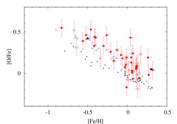
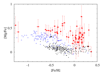
Figure 6: [O/Fe] (from Zoccali et al. 2006) and [Mg/Fe] against [Fe/H] for our sample of bulge giants (red circles) compared with the thin disk (blue triangles) and the thick disk samples (black squares) from Reddy et al. (2006) and Bensby et al. (2004, 2005). The black upwards and downwards pointing triangles are Arcturus and $\mu$Leo respectively. In the [O/Fe] panel, only Bensby et al. (2004) [OI] measurements are shown. Notice the clear separation between the thin disk, thick disk and bulge stars.

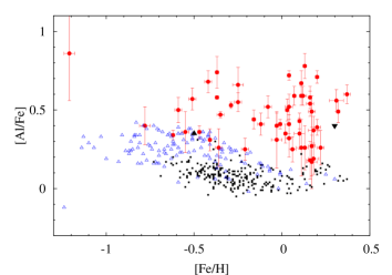
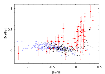
Figure 7: [Na/Fe] and [Al/Fe] ratio against [Fe/H] for our sample. Symbols as in figure 6

In this section we consider the resulting O, Mg, Na and Al abundances obtained for our bulge sample, and compare them with galactic thin and thick disk abundances taken from the studies of Reddy et al. (2006) and Bensby et al. (2004, 2005). We also briefly compare our results with earlier works on the bulge stars: (i) the seminal work of McWilliam & Rich (1994) for 12 cool RGB stars studied at lower resolution (R$\sim$20000); (ii) the infrared spectral analysis of 14 bulge M giants from Rich & Origlia (2005), although this study has a small metallicity coverage, restricted to [Fe/H] between $-$0.3 and +0.0 dex; (iii) the preliminary results for $\sim$20 giants from Keck HIRES high resolution spectra comparable to our UVES spectra (O and Mg by Fulbright et al., 2005; McWilliam & Rich, 2004, for Al in a subset of 9 stars). All the above-mentioned stars were confined to Baade’s Window.

We have checked whether the stars in our four bulge fields could be separated in the various abundance ratios plots, but did not find any significant field-to-field difference. Therefore in the following we discuss the 53 stars as a single sample. We have also estimated the number of expected disk foreground contaminants in each of the 4 fields using the Besancon model of the Milky Way, double checked with the disk control field discussed in Zoccali et al. (2003). At the RGB level, the contamination percentage is 15% in all fields (it is even smaller at the level of the red clump), except for the one at b=$-$12 where it reaches 45%. According to this, and given the total number of observed stars in each field we should have 2 disk stars in each of the 4 fields. In fact, in the most contaminated field (b=$-$12), we have identified two objects for which the ionization balance of iron was totally off, and furthermore showed pressure broadened wings in strong lines that clearly identified these two stars as disk foreground dwarf and subgiant respectively. These two stars were rejected from the final sample. In the other fields, we could not identify any other such clear-cut foreground star, but it should be kept in mind that, of the remaining 53 objects in our sample, 6 might be disk contaminants.

5.1 Observed trends in the bulge

The two elements with even atomic number O and Mg show a very similar trend (Fig. 6), with a decline of the overabundance with respect to iron as the metallicity increases (much shallower for magnesium than for oxygen). This behaviour is qualitatively similar to that found in previous studies of the galactic bulge. In particular, within the limited metallicity coverage of Rich & Origlia (2005), both O and Mg are in good agreement, but there are appreciable differences with respect to Fulbright et al. (2005): (i) Fulbright et al. (2005) have systematically lower [O/Fe] values by $\sim$0.15 dex in the whole metallicity range. Part of this effect (0.05 dex) is due to differences in the adopted solar O abundance and [OI] line $\log\,gf$ (cf. Zoccali et al., 2006). The residual systematic difference amounts to $\sim$0.1dex, but the behaviour of [O/Fe] with metallicity is similar in the two studies (same slopes). Furthermore, Fulbright et al. (2006, private communication) now find the same small offset between galactic disks and bulge stars as we do (Zoccali et al., 2006). (ii) Although the [Mg/Fe] in metal-poor stars agree within 0.1 dex between the two studies (including the reference stars Arcturus), the metal-rich end differs in that our sample includes stars with a whole range of different Mg abundances, whereas the smaller statistics for [Fe/H]$>$0.0 in previous studies did not allow to see this effect. As a result, the radical difference between the behaviour of [O/Fe] and [Mg/Fe] seen by Fulbright et al. (2005) and McWilliam & Rich (2004) is somewhat reduced, although we also do see a declining [O/Mg] abundance at high metallicities, which does not appear to be predicted by current metallicity-dependent yields of massive stars (see Sect. 7).

Compared to $\rm\alpha$-elements, the two elements with odd atomic number Na and Al show a different behaviour (Fig. 7). Both [Na/Fe] and [Al/Fe] trends are rather flat up to [Fe/H]$\sim$0.0, at which point the [Na/Fe] ratios start increasing sharply with increasing metallicity, while Al seems to follow the Mg trend, with an increased dispersion and shallower (if any) decline. Sodium is only available in bulge giants from the study of McWilliam & Rich (1994), who also found high Na abundances ([Na/Mg]$\sim$0.5) for supersolar metallicity stars.

One of the other striking feature of the [Na/Fe] ratio in our sample is the sudden blow-up of the dispersion at the highest metallicities ([Fe/H]$\geq$+0.1): for example, while the dispersion of [Na/Fe] at metallicities below solar is of the order of 0.14 dex, compatible with the internal uncertainties on the abundance measurement alone (0.14 dex), the scatter increases to 0.29 dex for [Fe/H]$>$0, with a range of [Na/Fe] from $-$0.1 to almost +1.0. To make sure this effect is real, we investigated possible measurements errors, in particular since at the metal-rich end, internal uncertainties are larger due to the presence of weak CN lines in most of the wavelength domain. However, we could find no source of random uncertainty that could amount to such a large factor: observational errors are of 0.18 dex in the mean in the supersolar metallicity regime, and of stellar parameters uncertainties, temperature has the most impact on [Na/Fe] with an effect of +0.1 dex for an increase of 200K. We shall return to this point in Sect. 6.

We find high [Al/Fe] ratio for all stars of the sample, $\sim+0.5$ for stars with $\rm[Fe/H]<0$, and a larger dispersion around the same mean value for $\rm[Fe/H]>0$. Within uncertainties, this is compatible with the constant overabundance of $\rm[Al/Fe]\sim 0.3$ found by McWilliam & Rich (2004), although once again our larger sample allows to see the high dispersion at high metallicities.

5.2 Comparison to the galactic disks

Also displayed in Figs. 6 and 7 together with our results for bulge stars are abundances of the galactic thin and thick disks from the studies of Reddy et al. (2006) and Bensby et al. (2004, 2005). Thanks to the good agreement between these works, no symbol distinction was made between the stars of these samples. Note that for oxygen, we chose to restrict our comparison to the Bensby et al. (2004) data points based on the [OI] lines only, to make sure that no systematics hampers the comparison (see Zoccali et al., 2006, for a detailed description of the systematics corrections applied to insure that our work is on the same scale as the galactic disks points). Note that the weak [OI] line could not be measured in our two most metal-poor stars; similarly, Bensby et al. (2004) data points also stop around $-$0.9 dex, the [OI] line being intrinsically weaker in the main-sequence stars of his sample.

As illustrated by Fig. 6, the bulge stars have O and Mg abundances distinct from those of galactic thin and thick disks (cf. Zoccali et al., 2006, for the case of oxygen). In particular, for $\rm[Fe/H]>-0.5$, bulge [Mg/Fe] values are higher than those of thick disk stars, which in turn are higher than those of thin disk stars. This effect is similar for Al (Fig. 7) where the separation between thin disk, thick disk and bulge is even wider. These tightly correlated O, Na, Mg, and Al enhancements suggest that (relatively) massive stars played a dominant role in chemical enrichment of the bulge, thus strengthening the conclusion by Zoccali et al. (2006) –based on oxygen alone– that the bulge formed on a shorter timescale compared to the galactic disks.

On the other hand, as illustrated by Fig. 7, for $\rm[Fe/H]<0.0$, no clear separation is apparent between the [Na/Fe] ratios of thin disk, thick disk, and bulge stars. For $\rm[Fe/H]>0$, the [Na/Fe] trend increases strongly in the bulge stars; Bensby et al. also found an increase of [Na/Fe] in the disk, but of a much smaller amplitude. Therefore, despite the dispersion, a clear separation between bulge and galactic disks stars is apparent in that metallicity range.

It is worth noting that also the local disk clump star $\mu$Leo has very high [Na/Fe] and [Al/Fe] ratios, at odds with the main-sequence stars of disk samples. Specifically, the high $\mu$Leo Na and Al abundances were reported by Gratton & Sneden (1990); Smith & Ruck (2000) ([Na/Fe]=+0.56 and +0.44 respectively to be compared to our +0.50; and [Al/Fe]=+0.40 to be compared to our +0.40 dex). In the next section, we examine whether the Na and/or Al abundances in our evolved red giants could be affected by internal mixing in the stars themselves.

6 Mixing and the abundance of O, Na and Al

If the large Na (and Al) abundances found in our sample were a result of internal mixing processes along the RGB of the stars themselves, then these abundances would not reflect anymore the ISM abundances at the star’s birth, and therefore could not be used as tracers for the bulge formation process.

It is well established, both observationally and theoretically, that C and N abundances evolve along the RGB, due to internal mixing of CN-cycled material, visible in particular in the ¹³C and ¹⁴N increase at the expense of ¹²C above the RGB bump luminosity (Lambert & Ries, 1981; Gratton et al., 2000; Charbonnel, 1994). Hence, some degree of mixing does indeed occur along the RGB. In search for probes of internal mixing for our bulge stars, we checked for a C-N anticorrelation, even though the C and N abundances are determined with a rather low accuracy ($\pm$0.2, but with nitrogen highly dependent on the derived carbon abundance since it is determined from the strength of the CN molecular bands). Within these uncertainties, we find no anticorrelation of [C/Fe] with [N/Fe], but merely a scatter entirely accounted for by measurement uncertainties. The [C/Fe] and [N/Fe] ratios of core He-burning red clump stars and RGB stars are indistinguishable, with dispersions around the mean of the order of 0.14 and 0.16 dex respectively, well within the uncertainties. The mean [C/Fe] and [N/Fe] values ($-$0.04 and +0.43, respectively) are compatible with mildly mixed giants above the RGB bump. The mixing seems less efficient than in metal-poor field giants, as expected from the decreasing mass of the C-depleted region above the $\mu$-barrier with increasing metallicity, as predicted in the mixing scenario proposed by Sweigart & Mengel (1979). However, mixing should reach far deeper layers than those where the CN-cycle operates for Na to be produced in major amounts by proton captures on ²⁰Ne and brought up to the stellar surface (see e.g., Weiss et al. 2000). Such a deeper mixing would necessarily engulf the ON-cycled layers of the stars, were virtually all O is converted to N, and therefore the Na enhancement should be accompanied by a net increase of C+N at the stellar surface. A modest Na enhancement, without concomitant increase of C+N, could nevertheness take place as a result of proton captures on ²²Ne, which take place in an outer layer compared to the shell where O is converted to N (Weiss et al. 2000) . Indeed, the sum of the carbon and nitrogen abundances should stay constant if the C depletion and N enhancement that we are witnessing are the result of the dredge up of only CN cycled material, and instead should increase by a factor up to $\sim 3$ if also ON-cycled material is brought up to the surface. By good fortune the [C+N/Fe] ratio suffers much smaller observational uncertainties than the individual C and N measurements, and Fig. 8 shows its run with metallicity. Indeed, [C+N/Fe] is flat, with no evidence of scatter ($<[$C+N/Fe]$>=0.11\pm 0.10$), nor any difference between the red clump and RGB stars. (The two stars lying above the trend are the two C-rich stars mentioned above.) Since much of the deep mixing should take place along the upper RGB, hence prior to the red clump phase, we can safely conclude that in the bulge stars deep mixing does not penetrate below the CN-cycled layer, hence no sodium or aluminium surface enhancement has taken place within these stars themselves. We also note that the [C+N/Fe] in the bulge giants is very similar to the carbon abundance in the galactic thin and thick disks Bensby & Feltzing (2006).

6.1 Correlations and Anticorrelations

Still, when [O/Fe] is plotted against [Na/Fe] (Fig. 9), an anticorrelation appears, reminiscent of the O-Na and Mg-Al anticorrelations found in globular clusters, where it is thought to reveal material polluted by $p-$capture on Ne to produce Na, and on Mg to produce Al in hot H-burning regions (where O is depleted by ON cycling). Such anticorrelations have never been reported among field stars to date, and in clusters they are though to be due to a superimposition of mixing of CNO processed matter in the atmosphere of evolved stars and chemical enrichment within the cluster, although the culprits for this latter process are not yet well defined (Gratton et al., 2004). In our bulge giants sample, although the [Mg/Fe] versus [Al/Fe] plot does not reveal much more than scatter (Fig. 10), [Na/Fe] and [Al/Fe] are found to be very well correlated (Fig. 11), similar again to what is found in globular clusters. Given the homogeneity in C and N of our sample however, we think very unlikely that the O-Na anticorrelation arises from the same mechanisms as in globular clusters, where it is associated with large CN variations On the other hand, the bulge stars of our sample, contrary to globular cluster stars, have metallicities in a wide range, and the O-Na anticorrelation could be created by an opposite global run of these two elements with metallicity. In fact, for [Fe/H]$>-0.2$ the [O/Fe] ratio decreases from halo-like values towards a solar composition. To test whether the O-Na correlation could be the result of this simple [O/Fe] evolution alone, we also tested whether $\delta$O, defined as the distance of each star to the mean [O/Fe] versus [Fe/H] trend ($\delta$O=([O/Fe]- mean trend), also anticorrelates with [Na/Fe]. This is not the case anymore, since all the remaining scatter around $\delta$O is compatible with the sole random uncertainties on the measurement. We therefore conclude that the O-Na anticorrelation and Na-Al correlation are the result of the chemical evolution of the galactic bulge (see next section) and are not necessarily related to the O, Na, Mg, and Al anomalies seen in globular clusters.

Finally, let us note that Mishenina et al. (2006) reached the same conclusion about their solar neighborhood giants, namely, that their rather high Na abundances (reaching to [Na/Fe]=+0.3dex) could not be the result of internal mixing but rather reflected the composition of the ISM at formation. This is somewhat at odds with the lower Na abundances measured in solar neighborhood dwarfs (Bensby et al., 2005), so that we may have to consider possible systematics between Na measurements in dwarfs and giants. Nevertheless, in the metal-rich regime ([Fe/H]$>$0.0), in our bulge giants the Na abundances are clearly above those of the galactic disk, whether measured in dwarfs or giants.

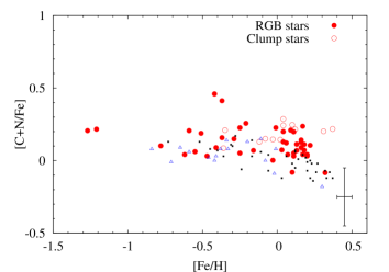
Figure 8: The run of [C+N/Fe] with metallicity is displayed for the sample stars (bulge symbols as in Fig. 9), overlapping with the [C/Fe] in the galactic thin (black squares) and thick (blue triangles) disks, as of Bensby & Feltzing (2006).

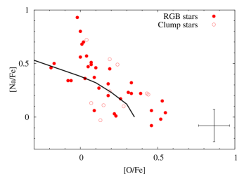
Figure 9: [Na/Fe] against [O/Fe] four our sample of bulge giants. No distinction can be made between red clump stars (open circles) and RGB stars (filled circles). The solid line indicates the locus of the general shape of the Na-O anticorrelation found in globular clusters (Carretta et al., 2006).

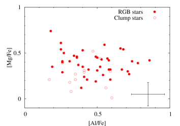
Figure 10: [Mg/Fe] against [Al/Fe] for our sample of bulge stars. Symbols as in Fig. 9. No anticorrelation is seen in this plane.

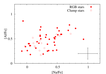
Figure 11: Correlation of [Al/Fe] against [Na/Fe] for our sample of bulge stars. Symbols as in Fig. 9.

7 Massive stars nucleosynthesis and the bulge formation

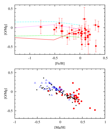
Figure 12: Run of the [O/Mg] ratio with metallicity for the bulge stars of our sample (circles). On the top panel, the predicted yields for SN II of 15M_⊙ (full line), 20M_⊙ (dashed line), 25M_⊙ (dotted line) and 35M_⊙ (dash dotted line) from Chieffi & Limongi (2004) are overlaid on the [O/Mg] versus [Fe/H] abundances. On the bottom panel, the bulge is compared to the galactic thin (black squares) and thick (blue triangles) disks, as of Bensby et al. (2004), using [Mg/H] as a proxy for metallicity.

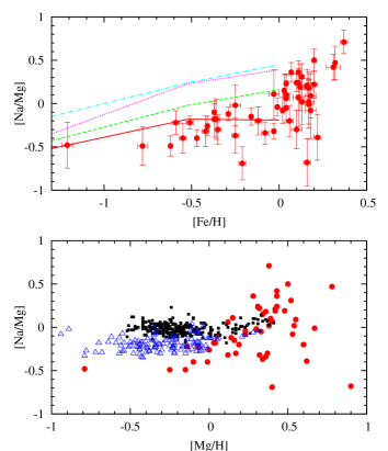
Figure 13: Top panel: run of the [Na/Mg] ratio with [Fe/H] for the bulge stars of our sample. Symbols as in Fig. 12. On the bottom panel, the bulge is compared to the galactic thin and thick disks as of Bensby et al. (2005) and Reddy et al. (2006), using [Mg/H] as a proxy for metallicity.

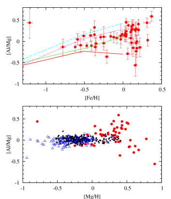
Figure 14: Top panel: run of the [Al/Mg] ratio with [Fe/H] for the bulge stars of our sample. Symbols as in Fig. 12. On the bottom panel, the bulge is compared to the galactic thin and thick disks as of Bensby et al. (2005) and Reddy et al. (2006), using [Mg/H] as a proxy for metallicity.

While using iron as a reference element has the advantage of minimizing random uncertainties (because of the large number of available lines), it is not the best choice to investigate the metal production by massive stars, since iron is produced both by SNII’s and SNIa’s. We have therefore investigated the interrelations of O, Na, Mg and Al, without reference to iron, to best probe the massive stars responsible for the enrichment of the bulge in these elements. Let us note once more that all four elements are produced in the hydrostatic phase of massive stars, hence largely independent of the explosion mechanism and mass cut which introduce large uncertainties on the yields of some other elements by SNII’s. While the production of O and Mg are expected to be going in lockstep, with no metallicity dependance of their relative yields, the synthesis of Al and Na on the contrary is expected to be more efficient with increasing neutron excesses, i.e. when the metallicity of the SNII progenitor increases. Thus we plot in Fig. 13 and 14 the Na/Mg and Al/Mg ratios as a function of [Fe/H] when comparing the observed abundances and theoretical yields, as the neutron donor elements may follow more closely Fe rather than Mg.

As mentioned in the introduction, sizable amounts of Na and Al can also be produced by intermediate-mass stars experiencing the envelope burning process while on the AGB. The timescale for the release of these elements by such stars will range from $\sim 30$ Myr (the lifetime of a $8\,$$M_{\odot}$ star) to $\sim 200$ Myr (the lifetime of a $4\,$$M_{\odot}$ star). Therefore, the release of Na and Al by massive and intermediate-mass stars will take place within the first $\sim 200$ Myr past an episode of star formation, with the release from SNII’s taking place on a timescale much shorter than that of bulge formation, and that from AGB stars on a timescale that may be comparable to it. In the following we compare the data only to the theoretical yields from massive stars, as the efficiency of the envelope burning process in AGB stars is extremely model dependent, and so is the production of Na and Al.

Figs. 12, 14 and 13 show the abundance ratios of O, Al and Na relative to Mg for our bulge sample (red clump and RGB stars). In the bottom panel of each figure, the Bulge is compared to the galactic disks (thin and thick) as of Bensby et al. (2005) and Reddy et al. (2006), using Mg as a metallicity proxy (i.e. as a function of [Mg/H]). In this way, Bulge and disks can be compared without reference to the SNIa which have heavily contributed to the disk Fe enrichement. Also shown in these figures (top panel of each figure) are the predicted yields of SNII from Chieffi & Limongi (2004, hereafter CL04), as a function of [Fe/H]. We have also considered the yields from Woosley & Weaver (1995, hereafter WW95) study but Mg appears to be under-produced by these models (Timmes et al. (1995)). Since we use Mg as a reference element, we display only the CL04 yields.

Some clear trends are apparent among these abundance ratios:

a) The [O/Mg] ratio decreases with increasing metallicity (whether probed by Fe or Mg), from close to solar down to $\sim-$0.3 for the most metal-rich stars (Fig. 12). Indeed, a slope of $-0.45\pm 0.18$ is found in the [O/Mg] versus [Mg/H] plane, with the dispersion being compatible with the measurement uncertainties. For [Mg/H] $<$ 0.4, the thin disk, the thick disk and the bulge lie on the same sequence (within the uncertainties). At higher [Mg/H] values, the bulge extends this trend to even lower [O/Mg] values. On the upper panel of Fig. 12, the [O/Mg] decrease is stronger than that predicted by either the CL04 or the WW95 yields, which both are almost independent of metallicity. An even stronger decline of [O/Mg] with metallicity has been reported by Fulbright et al. (2005); McWilliam & Rich (2004), who tentatively attributed such low oxygen to the decrease of the effective progenitor mass due to more efficient winds at higher metallicity. Indeed, if a major amount of carbon is lost in a Wolf-Rayet (WC) wind, then it escapes being turned into oxygen and the oxygen yield is reduced. However, by the same token one may expect that also the Mg yield is reduced, and therefore it remains unclear whether stronger winds and associated formation of Wolf-Rayet stars would favor Mg over O, or vice-versa, and whether Na and Al production could also be affected. We can just note that part of the [O/Fe] decrease with [Fe/H] may be due to a decrease of the O yield with increasing SNII metallicity (as suggested by these observations but not predicted by theory), rather than be due exclusively to the late SNIa Fe production.

b) The [Na/Mg] ratio increases dramatically both with increasing [Mg/H] or [Fe/H], from -0.4 at low metallicity to +0.4 at high metallicity (Fig. 13). The abundances found in the bulge stars are lower than the predicted yields of CL04, in particular at low [Fe/H]. This has already been shown to be the case in more metal poor stars (Cayrel et al., 2004). Let us note that WW95 predict lower Na yields and would not have suffered this problem. However, the metallicity dependence of the massive star CL04 yields correctly matches the slope of the observed points. Moreover, note that [Na/Mg] values differ systematically in the bulge, in the thick and thin disks, with their average increasing from the bulge, to the thick disk, to the thin disk, ordered in accordance with their respective formation timescale. This systematic increase of [Na/Mg] from bulge to thick disk to thin disk suggests that a contribution other than that of short-lived massive stars may actually be at work, with AGB stars being the obvious candidate. S-process neutron-capture (Ba, Y, … ) elements could be used in conjunction with Na to establish this.

c) For [Fe/H] $<0.1$, the [Al/Mg] ratio is well predicted by the metallicity dependence of the yields of stars 20–35 $M_{\odot}$) (Fig. 14): the [Al/Mg] ratio increases with [Fe/H] with a slope of $\rm 0.36\pm 0.07$. Except for three outliers ( $>2.5\sigma$ away from the trend), the dispersion around this slope is compatible with the measurement uncertainties. For [Fe/H]$>0.1$ (or [Mg/H] $>0.4$), the [Al/Mg] ratio is more dispersed so the overall behaviour is more difficult to establish: a continuing rise of [Al/Mg] cannot be excluded within uncertainties, but neither a change of trend, such as a flattening or even a decrease. Let us note that no theoretical yields are available at these high metallicities. At low metallicity ([Mg/H] $<0$), the bulge, the thin and thick disk distributions appear to be merged. At higher metallicity, the bulge data are remarkably more dispersed, which may entirely be due to observational error. We conclude that, contrary to the case for the [Na/Mg] ratio, no clear bulge-disk difference exists, and that no additional Al production is required over that of massive stars. This suggests that the contribution by AGB stars may be important for Na but not for Al, possibly because of the higher temperature required to sustain the Mg-Al cycle compared to the Ne-Na cycle.

8 Conclusions

We have reported the abundances of the elements O, Na, Al and Mg in a sample of 53 bulge giants (13 in the clump and 40 on the RGB), in four fields spanning the galactic latitude between -3 and $-12^{\circ}$. Special care was taken in the analysis of the sample stars, in particular in performing a differential analysis with respect to the metal-rich giant $\mu$Leo which resembles best our bulge stars. Our main conclusions can be summarized as follows.

(i) The bulge oxygen, magnesium and aluminum ratios relative to iron are higher than those in both galactic disks (thin and thick) for [Fe/H]$>-0.5$. This abundance patterns point towards a short formation timescale for the galactic bulge leading to a chemical enrichment dominated by massive stars at all metallicities. A flatter IMF would be an alternative possible explanation for the Bulge high O, Mg and Al abundance. However, current theory does not predict with enough confidence the amount of iron produced by core-collapse SNae, owing to the difficulty in locating the mass cut between remnant and ejecta, which primarily affects the predicted iron yield. Hence, it remains conjectural that flatter IMF implies an alpha enhancement.

(ii) The bulge stars have O/Mg and Al/Mg ratios similar to those of the galactic disk stars of the same metallicity, thus confirming that the enrichment of these elements is dominated by massive stars in all three populations.

(iii) In the bulge stars the [O/Mg] ratio follows and extends to higher metallicities the decreasing trend of [O/Mg] found in the galactic disks. This is at variance with current theoretical O and Mg yields by massive stars which predict no metallicity dependence of this ratio.

(iv) The trend of the [Na/Mg] ratio with increasing [Mg/H] is found to split in three distinct sequences, with [Na/Mg] in the thin disk being above the value in the thick disk, which in turn is above the bulge values. This hints for an additional source of Na from longer-lived progenitors (more active in the disk than in the bulge), with AGB stars more massive than $\sim 4\,$$M_{\odot}$  being the most plausible candidates. Indeed, the envelope burning process in these stars is expected to activate the Ne-Na cycle, hence producing sizable amounts of sodium.

(v) Contrary to the case of the [Na/Mg] ratio, there appears to be no systematic difference in the [Al/Mg] ratio between bulge and disk stars, and the theoretical yields by massive stars agree with the observed ratios. This suggests that the maximum temperatures reached in AGB stars experiencing the envelope burning process may not be sufficiently high to ignite also the Mg-Al cycle.

In the future we expect to extend our study of detailed abundances in our bulge sample by probing also heavier elements: heavier $\alpha$-elements (Si, Ca, Ti), iron peak and neutron capture elements (Ba, Eu), thereby revealing further characteristics of the bulge chemical enrichment and formation process.

Table 6: Abundances of Fe, O, Mg, Al, Na, C and N for the program stars. The flag column describes the quality of the O measurement: 0=good measurement; 1=uncertain measurement due to telluric lines in the vicinity or bad quality fit; 2=no measurement

Star	[Fe/H]	$\sigma$	[O/Fe]	Flag	[Mg/Fe]	$\sigma$	[Al/Fe]	$\sigma$	[Na/Fe]	$\sigma$	[C/Fe]	[N/Fe]
	dex	dex	dex		dex	dex	dex	dex	dex	dex	dex	dex
BWc-1	0.04	0.01	0.19	0	0.29	0.12	0.41	0.06	0.24	0.08	0.12	0.50
BWc-2	0.02	0.01	0.07	0	0.21	0.12	0.35	0.06	0.13	0.09	-0.09	0.52
BWc-3	0.31	0.04	0.19	0	0.12	0.09	0.56	0.07	0.54	0.12	0.04	0.51
BWc-4	-0.08	0.02	0.28	0	0.44	0.10	0.52	0.07	0.10	0.08	0.06	0.36
BWc-5	0.37	0.02	0.04	0	0.01	0.10	0.60	0.06	0.72	0.09	-0.01	0.59
BWc-6	-0.35	0.02	0.43	0	0.52	0.15	0.47	0.02	0.22	0.08	-0.20	0.69
BWc-7	-0.36	0.02	0.44	0	0.39	0.17	0.26	0.12	0.21	0.16	-0.20	0.50
BWc-8	0.17	0.03	-0.07	1	0.21	0.20	0.17	0.17	0.23	0.16	-0.22	0.47
BWc-9	0.04	0.02	0.11	1	0.08	0.22	0.32	0.12	0.14	0.16	-0.13	0.77
BWc-10	-0.12	0.02	0.15	0	0.31	0.11	0.41	0.07	0.11	0.12	-0.15	0.54
BWc-11	-0.03	0.03	9.99	2	0.18	0.22	0.31	0.18	0.29	0.18	-0.14	0.56
BWc-12	0.12	0.02	0.24	0	0.30	0.21	0.59	0.06	0.49	0.17	0.19	0.29
BWc-13	0.10	0.03	0.13	0	0.27	0.13	0.35	0.10	-0.03	0.18	0.12	0.51
B6-b1	0.07	0.01	0.04	1	0.21	0.07	0.59	0.06	0.57	0.09	-0.16	0.39
B6-b3	0.10	0.01	0.19	0	0.21	0.06	0.43	0.05	0.45	0.08	-0.16	0.11
B6-b4	-0.41	0.01	0.53	0	0.41	0.09	0.31	0.07	0.15	0.07	-0.24	0.53
B6-b5	-0.37	0.01	0.33	0	0.42	0.08	0.58	0.01	0.32	0.06	-0.11	0.56
B6-b6	0.11	0.01	0.01	0	0.32	0.08	0.67	0.08	0.68	0.11	-0.03	0.57
B6-b8	0.03	0.01	0.10	0	0.31	0.14	0.50	0.07	0.46	0.12	0.08	0.05
B6-f1	-0.01	0.01	0.18	0	0.24	0.07	0.41	0.03	0.20	0.07	0.05	0.55
B6-f2	-0.51	0.02	0.39	0	0.44	0.07	0.57	0.07	0.22	0.03	-0.04	0.56
B6-f3	-0.29	0.01	0.18	1	0.43	0.06	0.53	0.02	0.31	0.05	-0.09	0.53
B6-f5	-0.37	0.01	9.99	2	0.41	0.12	0.74	0.10	0.23	0.17	0.37	0.53
B6-f7	-0.42	0.02	9.99	2	0.54	0.12	0.68	0.07	0.22	0.13	0.42	0.57
B6-f8	0.04	0.01	-0.17	0	0.27	0.08	0.72	0.03	0.50	0.08	-0.11	0.51
BW-b2	0.22	0.02	0.23	1	0.40	0.19	0.26	0.11	0.01	0.18	0.05	0.25
BW-b5	0.17	0.02	0.09	0	0.19	0.13	0.49	0.10	0.37	0.13	0.06	0.56
BW-b6	-0.25	0.02	0.33	0	0.59	0.15	0.55	0.06	0.22	0.14	0.05	0.55
BW-f1	0.32	0.01	-0.02	0	0.46	0.12	0.49	0.07	0.93	0.15	-0.26	0.24
BW-f4	-1.21	0.03	9.99	2	0.42	0.21	0.86	0.30	-0.06	0.16	0.04	0.54
BW-f5	-0.59	0.02	0.31	1	0.45	0.11	0.50	0.08	0.23	0.08	0.03	0.53
BW-f6	-0.21	0.02	0.46	0	0.61	0.14	0.25	0.07	-0.08	0.13	0.08	0.58
BW-f7	0.11	0.03	0.03	0	0.29	0.21	0.26	0.18	0.36	0.26	-0.10	0.30
BW-f8	-1.27	0.03	9.99	2	0.56	0.18	9.99	9.99	9.99	9.99	0.03	0.53
BL-1	-0.16	0.01	0.26	0	0.32	0.07	0.44	0.06	0.17	0.07	0.03	0.18
BL-2	disk contaminant
BL-3	-0.03	0.01	0.22	0	0.35	0.07	0.40	0.08	0.03	0.06	-0.07	0.18
BL-4	0.13	0.01	0.02	1	0.39	0.09	0.78	0.08	0.70	0.12	-0.04	0.41
BL-5	0.16	0.01	0.07	0	0.32	0.07	0.58	0.07	0.51	0.07	0.04	0.33
BL-7	-0.47	0.01	0.46	0	0.46	0.05	0.36	0.04	0.06	0.08	-0.17	0.38
BL-8	disk contaminant
B3-b1	-0.78	0.03	0.55	0	0.53	0.15	0.40	0.12	0.04	0.16	-0.10	0.45
B3-b2	0.18	0.03	0.12	1	0.35	0.19	0.19	0.10	0.27	0.26	-0.13	0.42
B3-b3	0.18	0.03	-0.19	1	0.37	0.11	0.37	0.09	0.46	0.23	-0.09	0.46
B3-b4	0.17	0.02	0.07	0	0.50	0.24	0.27	0.19	0.49	0.13	-0.16	0.39
B3-b5	0.11	0.01	0.00	1	0.32	0.10	0.59	0.06	0.56	0.10	-0.15	0.40
B3-b7	0.20	0.02	-0.06	0	0.12	0.11	0.39	0.05	0.34	0.11	-0.16	0.39
B3-b8	-0.62	0.01	0.52	1	0.47	0.10	0.34	0.03	-0.02	0.06	-0.16	0.39
B3-f1	0.04	0.02	0.19	0	0.35	0.11	0.52	0.08	0.45	0.12	0.09	0.44
B3-f2	-0.25	0.03	9.99	2	0.55	0.21	0.66	0.11	0.53	0.11	-0.15	0.40
B3-f3	0.06	0.02	-0.08	1	0.54	0.11	0.25	0.08	0.34	0.14	-0.08	0.47
B3-f4	0.09	0.03	0.43	0	0.20	0.29	9.99	9.99	9.99	9.99	0.10	0.45
B3-f5	0.16	0.02	0.09	1	0.74	0.23	0.18	0.12	0.06	0.15	-0.06	0.49
B3-f7	0.16	0.02	0.05	0	0.26	0.14	0.54	0.08	0.47	0.12	-0.02	0.33
B3-f8	0.20	0.01	0.00	1	0.30	0.10	0.71	0.04	0.80	0.08	-0.17	0.38

Table 7: Abundances from individual Na and Al lines.

Star	[Al/Fe]	$\sigma$	[Al/Fe]	$\sigma$	[Na/Fe]	$\sigma$	[Na/Fe]	$\sigma$
	6696 $\AA$		6698 $\AA$		6154 $\AA$		6160 $\AA$
BWc-1	0.42	0.06	0.37	0.15	0.24	0.10	0.24	0.13
BWc-2	0.47	0.10	0.27	0.08	0.13	0.14	0.13	0.13
BWc-3	0.62	0.08	0.42	0.12	0.71	0.22	0.46	0.15
BWc-4	0.56	0.10	0.46	0.11	0.09	0.08	0.14	0.22
BWc-5	0.60	0.06	0.60	0.20	0.74	0.10	0.59	0.27
BWc-6	0.57	0.15	0.47	0.03	0.22	0.10	0.22	0.17
BWc-7	0.14	0.25	0.29	0.14	9.99	9.99	0.21	0.16
BWc-8	0.07	0.21	0.32	0.27	0.41	0.27	0.11	0.21
BWc-9	0.39	0.22	0.29	0.15	0.14	0.20	0.14	0.28
BWc-10	0.60	0.11	0.30	0.09	0.11	0.14	0.11	0.24
BWc-11	0.31	0.18	9.99	9.99	0.27	0.22	0.32	0.28
BWc-12	0.61	0.06	0.41	0.21	0.47	0.23	0.52	0.27
BWc-13	0.28	0.16	0.38	0.12	0.06	0.30	-0.09	0.24
B6-b1	0.62	0.07	0.52	0.10	0.63	0.12	0.48	0.15
B6-b3	0.43	0.07	0.43	0.08	0.51	0.12	0.41	0.10
B6-b4	0.35	0.14	0.30	0.08	0.15	0.11	0.15	0.09
B6-b5	0.63	0.06	0.58	0.01	0.29	0.09	0.34	0.07
B6-b6	0.67	0.12	0.67	0.11	0.68	0.14	0.68	0.20
B6-b8	0.54	0.08	0.39	0.13	0.39	0.17	0.54	0.18
B6-f1	0.49	0.07	0.39	0.04	0.20	0.08	0.20	0.14
B6-f2	0.57	0.11	0.57	0.09	0.25	0.06	0.20	0.04
B6-f3	0.62	0.08	0.52	0.03	0.30	0.06	0.35	0.08
B6-f5	0.96	0.16	0.61	0.12	0.12	0.23	0.37	0.26
B6-f7	0.80	0.11	0.60	0.09	0.21	0.15	0.26	0.27
B6-f8	0.81	0.10	0.71	0.04	0.50	0.10	0.50	0.14
BW-b2	0.26	0.13	0.26	0.21	-0.04	0.24	0.06	0.27
BW-b5	0.51	0.12	0.46	0.17	0.31	0.16	0.51	0.24
BW-b6	0.71	0.15	0.51	0.07	0.08	0.19	0.38	0.20
BW-f1	0.46	0.08	0.66	0.17	0.90	0.19	1.00	0.26
BW-f4	0.86	0.30	9.99	9.99	0.24	0.29	-0.21	0.20
BW-f5	0.46	0.15	0.51	0.09	0.20	0.12	0.25	0.10
BW-f6	0.33	0.15	0.23	0.08	-0.22	0.24	-0.02	0.16
BW-f7	0.26	0.18	9.99	9.99	0.36	0.26	9.99	9.99
BW-f8	9.99	9.99	9.99	9.99	9.99	9.99	9.99	9.99
BL-1	0.41	0.11	0.46	0.08	0.16	0.09	0.21	0.15
BL-2	disk contaminant
BL-3	0.46	0.12	0.36	0.11	0.01	0.09	0.06	0.10
BL-4	0.83	0.12	0.73	0.12	0.73	0.17	0.68	0.16
BL-5	0.61	0.08	0.51	0.12	0.56	0.11	0.46	0.11
BL-7	0.39	0.07	0.34	0.06	0.08	0.11	0.03	0.11
BL-8	disk contaminant
B3-b1	0.40	0.27	0.40	0.14	0.17	0.22	-0.13	0.24
B3-b2	0.25	0.11	-0.05	0.22	9.99	9.99	0.27	0.26
B3-b3	0.40	0.14	0.35	0.12	0.46	0.23	9.99	9.99
B3-b4	0.22	0.27	0.32	0.27	0.31	0.19	0.66	0.18
B3-b5	0.61	0.08	0.56	0.10	0.58	0.11	0.48	0.22
B3-b7	0.35	0.10	0.40	0.07	0.31	0.18	0.36	0.15
B3-b8	0.34	0.07	0.34	0.03	-0.02	0.09	-0.02	0.07
B3-f1	0.44	0.11	0.59	0.11	0.49	0.15	0.39	0.20
B3-f2	0.59	0.16	0.74	0.17	0.46	0.23	0.56	0.13
B3-f3	0.28	0.14	0.23	0.11	0.34	0.18	0.34	0.24
B3-f4	9.99	9.99	9.99	9.99	9.99	9.99	9.99	9.99
B3-f5	0.13	0.14	0.28	0.21	9.99	9.99	0.06	0.15
B3-f7	0.56	0.11	0.51	0.13	0.44	0.14	0.54	0.21
B3-f8	0.70	0.04	0.75	0.07	0.81	0.09	0.76	0.15