Probing variations in fundamental constants with radio and optical quasar absorption-line observations

Abstract

Nine quasar absorption spectra at 21-cm and UV rest-wavelengths are used to estimate possible variations in $x\equiv\alpha^{2}g_{\rm p}\mu$, where $\alpha$ is the fine structure constant, $g_{\rm p}$ the proton $g$-factor and $\mu\equiv m_{\rm e}/m_{\rm p}$ is the electron-to-proton mass ratio. We find $\langle\Delta x/x\rangle^{\rm weighted}_{\rm total}$ $=(0.63\pm 0.99)\times 10^{-5}$ over a redshift range $0.23\mathrel{\hbox to0.0pt{\lower 3.0pt\hbox{$\sim$}\hss}\raise 2.0pt\hbox{$<$}}z_{\rm abs}\mathrel{\hbox to0.0pt{\lower 3.0pt\hbox{$\sim$}\hss}\raise 2.0pt\hbox{$<$}}2.35$ which corresponds to look-back times of 2.7–10.5 billion years. A linear fit against look-back time, tied to $\Delta x/x$ $=0$ at $z=0$, gives a best-fit rate of change of $\dot{x}/x=(-0.6\pm 1.2)\times 10^{-15}{\rm\,yr}^{-1}$. We find no evidence for strong angular variations in $x$ across the sky. Our sample is much larger than most previous samples and demonstrates that intrinsic line-of-sight velocity differences between the 21-cm and UV absorption redshifts, which have a random sign and magnitude in each absorption system, limit our precision. The data directly imply that the average magnitude of this difference is $\Delta v_{\rm los}\sim 6$ km s^-1.

Combining our $\Delta x/x$ measurement with absorption-line constraints on $\alpha$-variation yields strong limits on the variation of $\mu$. Our most conservative estimate, obtained by assuming no variations in $\alpha$ or $g_{\rm p}$ is simply $\Delta\mu/\mu$ $=$ $\langle\Delta x/x\rangle^{\rm weighted}_{\rm total}$. If we use only the four high-redshift absorbers in our sample, we obtain $\Delta\mu/\mu$ $=(0.58\pm 1.95)\times 10^{-5}$, which agrees ($2\sigma$) with recent, more direct estimates from two absorption systems containing molecular hydrogen, also at high redshift, and which have hinted at a possible $\mu$-variation, $\Delta\mu/\mu=(-2.0\pm 0.6)\times 10^{-5}$. Our method of constraining $\Delta\mu/\mu$ is completely independent from the molecular hydrogen observations. If we include the low-redshift systems, our $\Delta\mu/\mu$ result differs significantly from the high-redshift molecular hydrogen results. We detect a dipole variation in $\mu$ across the sky, but given the sparse angular distribution of quasar sight-lines we find that this model is required by the data at only the 88 per cent confidence level. Clearly, much larger samples of 21-cm and molecular hydrogen absorbers are required to adequately resolve the issue of the variation of $\mu$ and $x$.

1 Introduction

The existence of extra spatial dimensions remains an open question in theoretical physics. The answer to this question is closely linked to attempts at super-unification, which has become a modern holy grail. In turn, the existence of extra spatial or temporal dimensions may be inferred by the detection of spatial or temporal variations in the values of coupling constants, such as the fine structure constant, $\alpha$ (see Uzan, 2003; Karshenboim et al., 2005, for reviews). This constant provides a measure of the strength of the electromagnetic interaction and is truly fundamental because it is dimensionless and thus independent of any system of units. Other such constants are the electron-to-proton mass ratio, $\mu$, the proton gyromagnetic factor $g_{\rm p}$, as well as the constant $x$ defined as

$$x\equiv\alpha^{2}g_{\rm p}\mu\ ,$$ (1)

which combines all three. Apart from the question of extra dimensions, any confirmed detection of a variation in the value of any of these ‘constants’ would in itself be a ground-breaking result. For example, in some popular models this variation is related to violation of the Principle of Equivalence.

There have been several attempts to constrain the variation of fundamental constants either experimentally or observationally. Atomic clocks (see e.g. Prestage et al., 1995; Sortais et al., 2001; Marion et al., 2003; Flambaum et al., 2004; Flambaum & Tedesco, 2006) and the Oklo nuclear reactor (Shlyakhter, 1976; Fujii et al., 2000; Flambaum & Shuryak, 2002; Olive et al., 2002; Lamoreaux & Torgerson, 2004) provide local, i.e. earthbound and relatively recent, $z\sim 0$, constraints. The cosmic microwave background provides constraints at $z\sim 1000$ (Landau et al., 2001; Avelino et al., 2001; Martins et al., 2002). Further constraints may be obtained from Big Bang Nucleosynthesis data (see e.g. Dmitriev et al., 2004).

However, one very promising way to detect such variations is astronomical spectroscopy of gas clouds which intersect the lines of sight to distant quasars. This technique allows one to obtain constraints essentially over all of the intermediate redshift range, which is crucial for probing variations with cosmic time. Additionally, results achieve very high precision, due to the advent of 10-m class telescopes equipped with state-of-the art high-resolution spectrographs, in particular Keck/HIRES in Hawaii and VLT/UVES in Chile.

In this type of work, the gas clouds probed are often damped Lyman $\alpha$ systems (DLAs). These systems have high neutral hydrogen column densities ($N_{\rm HI}\mathrel{\hbox to0.0pt{\lower 3.0pt\hbox{$\sim$}\hss}\raise 2.0pt\hbox{$>$}}10^{20}\ {\rm cm}^{-2}$) at precisely determined redshifts, thus providing excellent probes of the bulk neutral atomic hydrogen in the distant Universe. Furthermore, DLAs contain many different heavy elements which absorb in the rest-frame ultraviolet (for atomic species) or millimetre (for molecular species), giving rise to a multitude of absorption lines. With the latest generation of optical telescopes rest-frame ultraviolet lines can be observed with resolutions of the order of 6 km s^-1 so that redshifts can be determined to six significant digits. This is crucial as all methods using this type of data aim to detect small shifts induced by a possible variation of constants which are of different magnitude for different transitions.

Using such data, Dzuba et al. (1999) and Webb et al. (1999) developed the highly sensitive many-multiplet method and in a series of papers applied it to rest-frame ultraviolet atomic quasar absorption lines, obtained with Keck/HIRES. Their work provided evidence that $\alpha$ is smaller at redshifts $0.2<z<3.7$ at the fractional level of $\Delta\alpha/\alpha=(-0.57\pm 0.10)\times 10^{-5}$ (Webb et al., 1999; Murphy et al., 2001; Webb et al., 2001; Webb et al., 2003; Murphy et al., 2003; Murphy et al., 2004). After thorough investigation Murphy et al. (2001) and Murphy et al. (2003) ruled out a large range of known systematic effects. However the issue remains controversial after another group found no evidence for a change in $\alpha$ using VLT/UVES spectra ($\Delta\alpha/\alpha=(-0.06\pm 0.06)\times 10^{-5}$ for $0.4<z<2.3$, Chand et al., 2004; Srianand et al., 2004).

Strong constraints on variations in the electron-to-proton mass ratio, $\mu$, can also be obtained from optical quasar absorption studies (Thompson, 1975). The first confirmed molecular hydrogen quasar absorption line detections were obtained by Levshakov & Varshalovich (1985), and confirmed by Foltz et al. (1988). However, although the large number of H₂ transitions in the Lyman and Werner bands have different dependencies on $\mu$, making them useful probes of $\mu$-variation, unfortunately the relatively small fraction of DLAs in which H₂ is detected has limited this work so far (Varshalovich & Levshakov, 1993; Ivanchik et al., 2002; Ubachs & Reinhold, 2004; Ivanchik et al., 2005). Nevertheless, the recent study of two high signal-to-noise spectra has yielded hints that $\mu$ may have been smaller at redshifts between $\sim$2.5–3.1 (Reinhold et al., 2006) .

A potentially more sensitive approach is possible when, as well as rest-frame UV, rest-frame 21-cm absorption from cold neutral hydrogen is also detected. In such cases, variability of the constant $x$, defined above, can be investigated. Because the ratio of 21-cm to UV transition frequencies is proportional to $x$, it can be shown that, if both UV and 21-cm absorption occurs at the same physical location, the relative change in the value of $x$ between its value at redshift $z$ and its value in a terrestrial lab is related to the observed absorption redshifts for rest-frame 21-cm and UV, $z_{\rm 21}$ and $z_{\rm UV}$, according to

$$\Delta x/x\equiv\frac{x_{z}-x_{0}}{x_{0}}=\frac{z_{\rm UV}-z_{\rm 21}}{1+z_{\rm 21}}$$ (2)

(e.g. Tubbs & Wolfe, 1980). In addition, because $\mu$ enters in Equation 2 via the definition of $x$, results on the variation of $\mu$ may also be obtained, allowing completely independent tests of $\Delta\mu/\mu$ results obtained more directly from molecular absorption lines. However, application of this method is limited by the fact that there are only $\sim$18 DLAs for which absorption has been observed both in the optical and in the radio (Curran et al., 2005, contains a detailed list). Consequently, there is only a handful of results based on this method (Wolfe & Davis, 1979; Tubbs & Wolfe, 1980; Cowie & Songaila, 1995; Wolfe et al., 1981). Among these, a high-resolution spectrum from a 10-m class telescope is used only once and for a single object (Cowie & Songaila, 1995). Furthermore, there has been no attempt to apply this method to a sample consisting of more than one object. This is important for two reasons:

1. Any systematic effects due to spatial non-coincidence of hydrogen and heavy elements can only be detected if a sample of objects is used.

2. To detect any space-time variation of $x$, one needs several observations, covering a range in redshift and direction.

The first results from such an approach were briefly presented in Tzanavaris et al. (2005). In this paper we explain in detail how these results were obtained and extend our original sample of eight absorbers with a newly discovered 21-cm absorber. We have filled the gap in the literature by applying this method to a sample comprising all the best available 21-cm absorption data in conjunction with the highest-resolution UV data available. The sample is made up of nine absorption systems situated along the line of sight to nine quasars covering the absorption redshift range $\sim 0.23$ to $\sim 2.35$. The paper’s structure is as follows: In Section 2 we describe our data sample. We describe our methods and results in Section 3. Our results are discussed in Section 4.

2 Data

2.1 Data sample and reduction

Details of the data used in this work are given in Table 1 and are discussed below. Our data sample is made up of nine quasar absorption systems along the lines of sight to nine quasars. Each system shows both 21-cm and UV absorption (rest frame) along the line of sight to a different quasar. Rest-frame UV absorption is observed red-shifted in the optical region, and rest-frame 21-cm is observed red-shifted at longer radio wavelengths. In this paper we use the labels UV and 21-cm to distinguish the two types of observations that we use.

Figures 3 to 11 show the 21-cm and UV data registered to a common velocity scale. We note that all data have been corrected to the heliocentric frame.

2.1.1 Radio data

The original radio 21-cm absorption spectra were not available for this work, apart from the data for quasar Q0458$-$020 which were kindly provided by Art Wolfe. Therefore, we digitised the 21-cm plots from the literature (see the references in Table 1) using the dexter application (Demleitner et al., 2001), available at NASA/ADS for on-line scanned papers or, for PDF plots, the stand-alone version available at http://sourceforge.net/projects/dexter.

The initial step was to digitise each spectrum, obtaining flux/abscissa values. Then a linear wavelength scale was derived for, and assigned to, each spectrum by carefully measuring velocity or frequency points on the x-axis of the plot. This second step dominates the uncertainty in the zero-point of the velocity/frequency scale but is nevertheless not an important source of error. As an example, we digitised a postscript plot of the Si ii 1808 Å absorption feature obtained with Keck/HIRES and compared the resulting redshift to that obtained from the original data. The two redshifts differed by just $1\times 10^{-6}$. A very conservative upper limit on the absolute velocity/frequency uncertainty is given by half of the digitised pixel size in each case. We checked the maximum contribution this zero-point error could make to the final estimate for $\Delta x/x$ for each quasar and, in all cases, this was less than 25 per cent of the statistical-plus-systematic (i.e. increased) error bars illustrated in Fig. 1. We therefore stress that the digitisation process generally contributes a small uncertainty in comparing the 21-cm and UV absorption redshifts.

Redshift uncertainties and details of the observations and data reduction can be found in the references listed in Table 1. However, since no redshift uncertainty is given for the radio spectrum of Q1127$-$145 in Kanekar & Chengalur (2001b) we used the uncertainty from Kanekar & Chengalur (2001a), as these are the same observers, using the same instrument to perform a similar type of observation.

2.1.2 Optical (rest-frame UV) data

Optical (rest-frame UV) high-resolution echelle spectral data for eight of the nine quasars were taken from the European Southern Observatory’s (ESO’s) archive. These were originally observed with the UVES spectrograph on the Very Large Telescope (VLT). Data reduction was carried out with the ESO/UVES pipeline (Ballester et al., 2000), modified to improve the flux extraction and the wavelength calibration precision. Post-pipeline processing was carried out using the custom-written code uves popler . For each quasar, the extracted echelle orders from all exposures were combined to form a single 1-dimensional spectrum, with cosmic ray signatures being rejected by a sigma-clipping algorithm during the combination. A continuum was constructed by iteratively fitting a series of overlapping polynomials, rejecting discrepant pixels at each iteration until convergence. For one of the quasars (Q1331$+$170) we have also included the part of the absorption spectrum for Si ii 1808 Å from a Keck/HIRES observation, provided by Art Wolfe. This spectrum was reduced with the dedicated Keck/HIRES pipeline, makee , written by Tom Barlow.

For quasar Q0235$+$164 we digitised an absorption plot from Lanzetta & Bowen (1992) for a single heavy element species.

Table 1: Details of our data sample. There is one 21-cm/UV absorption system along each quasar sight-line. Column 1 is the quasar name and Column 2 its emission redshift. For the strongest component Column 3 gives the 21-cm absorption redshift. The uncertainty is given in parentheses and has been taken from the references shown in Column 4. The original 21-cm plots were also obtained from these references. However, the entries marked with $\dagger$ which refer only to the source of the 21-cm redshift uncertainty, whilst for the entry marked with $\ast$ there is no uncertainty in redshift in the literature (see text). Column 5 gives the mean absorption redshift and standard deviation on the observed mean for the strongest UV component. Column 6 gives the UV heavy element species observed in the optical with the number of transitions in parentheses, if more than one. Column 7 gives the source for the UV data. For data obtained from the ESO/UVES archive, the ESO program identification code is given in this column and the principal investigator of the program is given in the footnotes. For Q1331$+$170 we also used Si ii 1808 Å Keck/HIRES data provided by A. Wolfe. For quasar Q0235$+$164 we digitised an absorption plot from the literature for a single heavy element species.

hline Quasar	$z_{\rm em}$	$z_{\rm 21}$	21-cm	$\langle z_{\rm UV}\rangle$	ions	UV
Q0952$+$179	1.478	0.237803(20)	[1]	0.237818(6)	Mg i, Ca ii(2)	69.A-0371(A)a
Q1127$-$145	1.187	0.312656(50)	[2]	0.312648(6)	Ca ii(2), Mn ii(3)	67.A-0567(A)b, 69.A-0371(A)a
Q1229$-$021	1.038	0.394971(4)	[3]	0.395019(40)	Ca ii(2), Mn ii(3), Ti ii	68.A-0170(A)c
Q0235$+$164	0.940	0.523874(100)	[4]	0.523829(6)	Mg i	Lanzetta & Bowen (1992)
Q0827$+$243	0.941	0.524757(50)	[1]	0.524761(6)	Ca ii(2), Fe ii	68.A-0170(A)c, 69.A-0371(A)a
Q1331$+$170	2.097	1.776427(20)	[5]	1.776355(5)	Mg i, Al ii, Si ii, S ii,	67.A-0022(A)d, 68.A-0170(A)c
					C i(3), C i∗, Cr ii(2), Mn ii(2),
					Fe ii(4), Ni ii(6), Zn ii
					Si iie	$\dagger$
Q1157$+$014	1.986	1.943641(10)	[6]	1.943738(3)	Mg i, Mg ii(2), Si ii,	65.O-0063(B)f, 67.A-0078(A)f,
					Ni ii(6)	68.A-0461(A)g
Q0458$-$020	2.286	2.039395(80)	[7]	2.039553(4)	Zn ii(2), Ni ii(6), Mn ii(3),	66.A-0624(A)f, 68.A-0600(A)f,
					Cr ii(3)	072.A-0346(A)f, 074.B-0358(A)h
Q0438$-$436	2.347	2.347488(12)	[8]	2.347403(49)	Zn ii(2), Mn ii, Fe ii, Si ii	69.A-0051(A)i, 072.A-0346(A)f

1: Kanekar & Chengalur (2001a); 2: Kanekar & Chengalur (2001b); uncertainty in redshift not available (see text); 3: Brown & Spencer (1979); 4: Wolfe et al. (1978); 5: Wolfe & Davis (1979); A. Wolfe, private communication: postscript plot; 6: Wolfe et al. (1981); 7: Wolfe et al. (1985); A. Wolfe, private communication: original data; 8: Kanekar et al. (2006).

$a$: Savaglio; $b$: Lane; $c$: Mallén-Ornelas; $d$: D’Odorico; $e$: Same transition as in the UVES data but from Keck/HIRES; $f$: Ledoux; $g$: Kanekar; $h$: Dessauges-Zavadsky; $i$: Pettini; $\dagger$ A. Wolfe, private communication: original Si ii data in Q1331$+$170.

3 Analysis

There is one absorption system for each 21-cm/UV absorption spectrum pair in a single quasar. To apply Equation 2 we need values for $z_{\rm UV}$ and $z_{\rm 21}$. We now explain how we chose these values.

3.1 Assumptions

In each absorption system we used the frequency or wavelength of strongest absorption for each absorbing species, neutral or singly ionised, to provide the 21-cm and UV redshifts. We justify these choices below but note that they need not represent the true physical picture for our results to be useful. Rather, they are used as a starting point for our analysis.

3.1.1 Strongest absorption

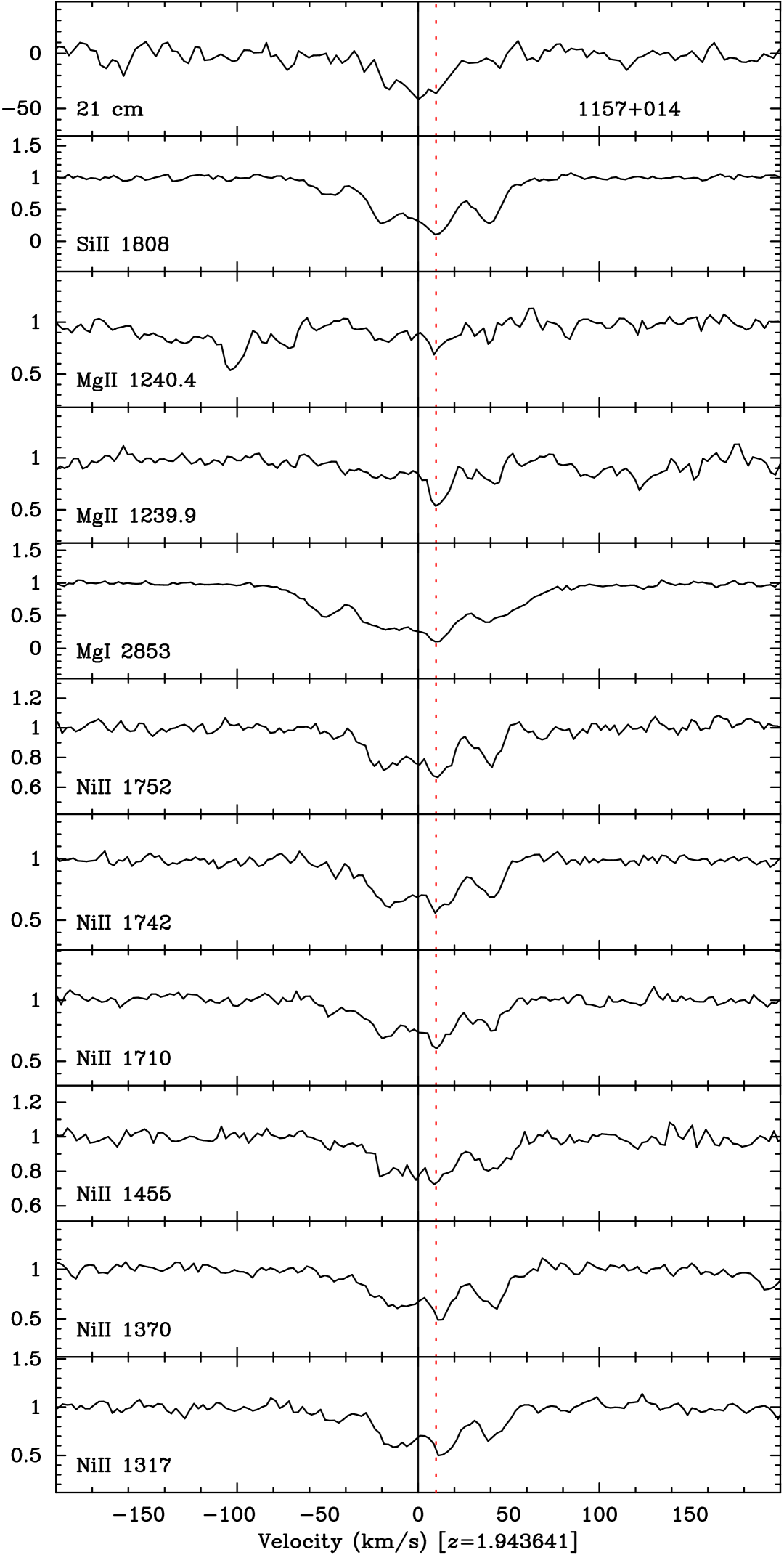
Figure 9: Velocity plot for 21-cm and UV absorption towards quasar Q1157$+$014. The 21-cm data are in units of flux density (mJy) after subtraction of a polynomial baseline. The UV data are continuum normalised. The solid vertical line at 0 km s^-1 is at $z_{\rm 21}$. The dotted vertical line is at $\langle z_{\rm UV}\rangle$.

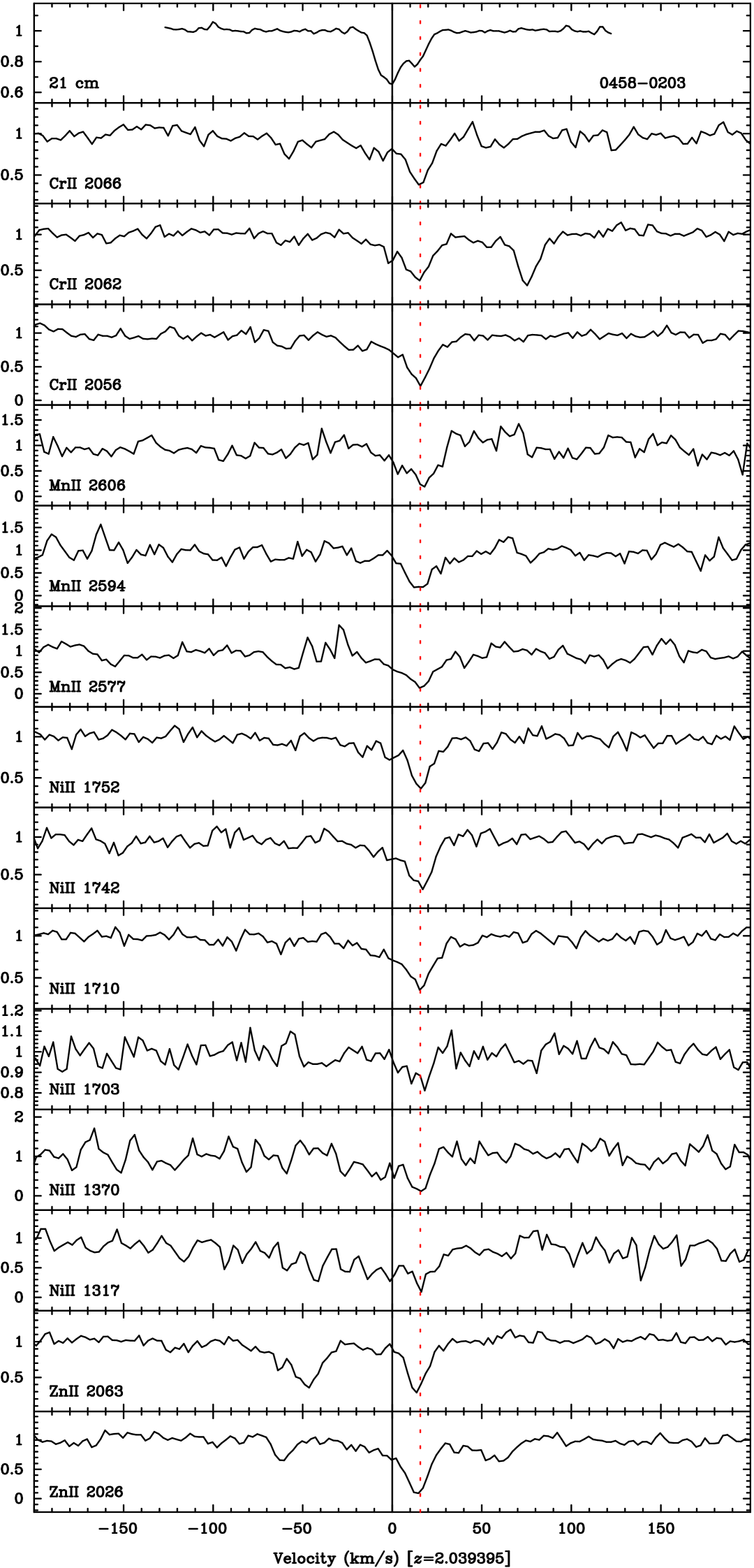
Figure 10: Velocity plot for 21-cm and UV absorption towards quasar Q0458$-$020. Both 21-cm and UV data are continuum normalised. The solid vertical line at 0 km s^-1 is at $z_{\rm 21}$. The dotted vertical line is at $\langle z_{\rm UV}\rangle$.

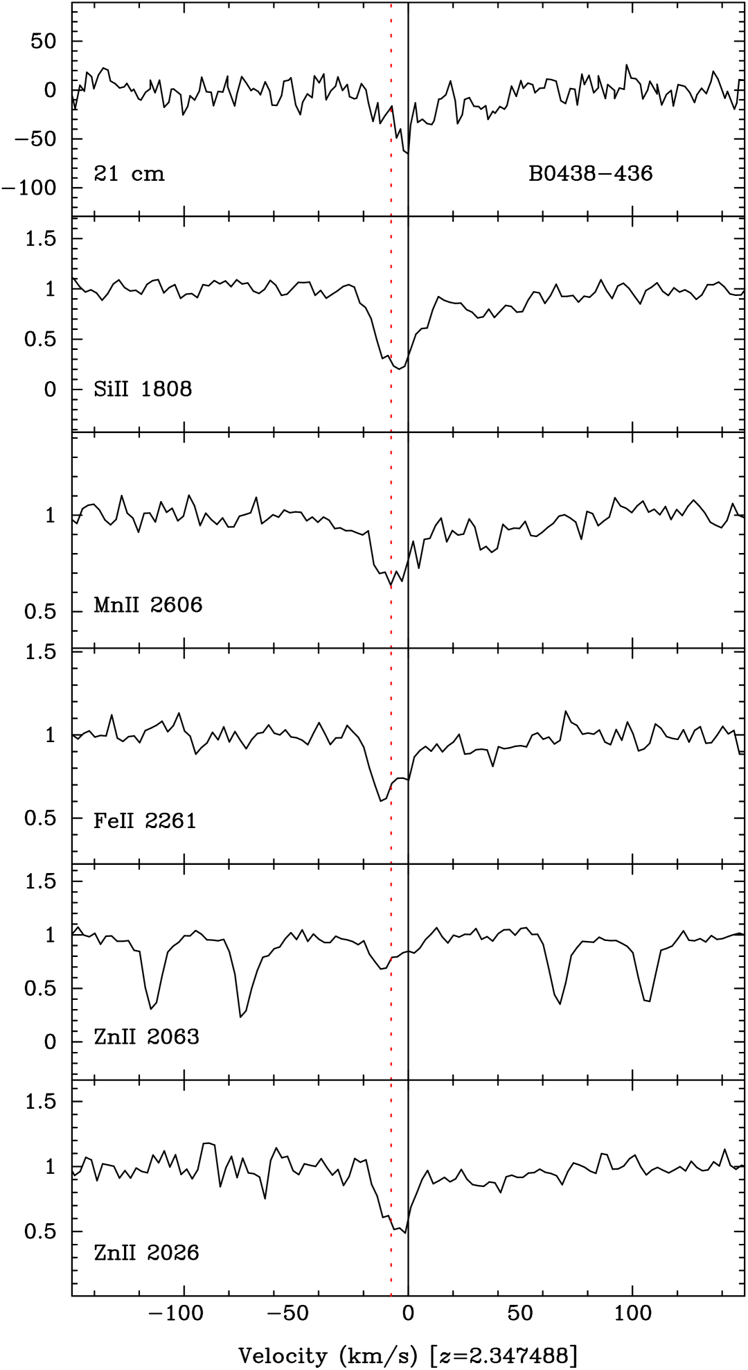
Figure 11: Velocity plot for 21-cm and UV absorption towards quasar Q0438$-$436. The 21-cm data are in units of flux density (mJy) after subtraction of a polynomial baseline. The UV data are continuum normalised. The solid vertical line at 0 km s^-1 is at $z_{\rm 21}$. The dotted vertical line is at $\langle z_{\rm UV}\rangle$.

It is evident from Figs. 3–11 that in most absorption systems there is usually complex velocity structure. For neutral and singly ionised heavy element species there is sufficient similarity in this structure so that corresponding components can be identified. Unfortunately, this is not normally the case when one compares UV to 21-cm absorption profiles in the same system. In other words, it is not easy to tell which 21-cm absorption component corresponds to which UV absorption component. However, a decision must be made because Equation 2 only holds if it is applied to 21-cm and UV redshifts for components which are situated at the same physical location. It is important to realise that this represents a fundamental limitation in the comparison of 21-cm and UV absorption lines when deriving constraints on varying constants. Clearly, this problem can only be overcome using a statistically large sample of absorption systems. The method used to determine the ‘centroid’ of the 21-cm and UV absorption is also clearly not crucial provided that it is unbiased and that uncertainties can be reliably estimated.

Given the inherent dissimilarity between the 21-cm and UV absorption profiles, many possible methods exist for choosing appropriate 21-cm and UV redshifts. For example, for a single absorber, the various UV profiles might be cross-correlated with the 21-cm profile or one might attempt to identify ‘nearest neighbour’ UV and 21-cm velocity components. However, for the cross-correlation example, it is not clear how to derive a meaningful uncertainty on the redshift comparison. In the ‘nearest neighbour’ approach, recently advocated in Kanekar et al. (2006), a detailed fit to the 21-cm and UV profiles is required to identify all the velocity components and, given the general variety of spectral resolutions apparent in Figs. 3–11, this is difficult. Moreover, this approach is strongly biased towards zero $x$-variation and this bias is again resolution-dependent. The redshift uncertainty for individual absorbers will therefore be too large. Similarly, for a large sample, the scatter in the values of $\Delta x/x$ will be significantly underestimated and any additional scatter caused by intrinsic velocity shifts between the 21-cm and UV components will be masked.

The simplest method is to take $z_{\rm 21}$ and $z_{\rm UV}$ from the strongest absorption component, as this is well-defined in our data. Although there is no general similarity in the velocity profiles, we assume that strongest absorption occurs at the same physical location for all species. We stress that this is a simple, initial assumption and later we demonstrate that we can actually use our results to test this assumption. Given the range of options above and given the fundamental limitation in associating 21-cm and UV components which are typically spaced by several km s^-1, it is also clear that detailed fits to the components in order to decrease the centroid position uncertainty to the sub-pixel level is unimportant. A cruder and simpler measurement, such as taking the redshift of the pixel with minimum intensity, will still involve an uncertainty which is smaller than the errors involved in comparing the 21-cm and UV profiles.

3.1.2 Neutral and singly ionised species

Neutral heavy element species might be considered more likely to be spatially coincident with 21-cm absorbing gas, which is due to neutral hydrogen. We decided to use singly ionised species as well for the following reasons:

1. In our sample, the velocity structure of neutral species was followed closely by singly ionised species. This was also true in the much larger sample in Murphy et al. (2004) used to constrain variations in $\alpha$.

2. Extensive work by Prochaska (2003) more generally indicates that ionisation fraction, abundance and dust-depletion may not change significantly along an absorption complex.

3. In any case, we only used the simple option of strongest components and these, in the overwhelming majority of cases, corresponded very clearly between neutral and singly ionised species (see Figs. 3–11).

By using both neutral and singly ionised species, we obtained a significantly larger sample of UV lines for each absorber. This allowed us to investigate systematics for individual absorbers for the first time. Note though that there is one exception to our approach. This concerns Ca ii which has not been used in our analysis, although it is singly ionised and shown in the figures for illustration purposes only (but see Section 4). The reason for this is that the Ca ii ionisation potential, 11.871 eV, is such that one would not expect this species to trace neutral components well compared to the other singly ionised species used. Since DLAs have high neutral hydrogen column densities, one expects only photons with energies $<13.6$ eV to penetrate the radiation shielding gas envelope. Such photons would then be unable to ionise species such as Fe ii (ionisation potential 16.18 eV) or Mn ii (ionisation potential 15.64 eV), but they would still be able to ionise Ca ii. Thus all singly ionised species used, apart from Ca ii, are much more likely to be the dominant ionised species in an absorption system. For this reason we did not use this transition, just as we did not use higher ionisation species.

3.2 Redshift determination

In the spectral region covered by an absorption system, strongest absorption occurs at that point where the observed intensity is at a minimum. For each 21-cm absorption complex we thus identified and measured the dispersion coordinate, MHz or km s^-1, at the pixel of minimum intensity, from which we then obtained $z_{\rm 21}$. We then searched the optical data for heavy element absorption features close to the redshifts where there is 21-cm absorption. We thus identified a number of UV absorption features, some of which were due to neutral species and some due to multiply ionised species, with the majority due to singly ionised species. For all detected UV features, where (1) absorption was due to either neutral or singly ionised species and (2) there was little or no saturation, we again determined the value of the dispersion coordinate, Å or km s^-1, at the pixel of minimum intensity. We then determined the corresponding absorption redshift, $z_{\rm UV}$. When there were several UV transitions in a system, we carried out this procedure individually for each transition, e.g. independently for Zn ii 2026 and Zn ii 2062. In all, we used 31 different UV transitions. We present detailed velocity plots of all 21-cm and UV absorption components used in this work in Figs. 3–11. We include the Ca ii profiles in these plots for comparison, even though we did not use them to determine $z_{\rm UV}$. These plots are centred at $z_{\rm 21}$, indicated by the solid vertical line. In each absorption system we calculated $\langle z_{\rm UV}\rangle$, the average of all redshift values determined for single species, as explained above. This is shown by the dotted vertical line in Figs. 3–11.

3.3 $\Delta x/x$ Results

We have obtained $\Delta x/x$ results using three different methods. The methods and results are summarised in Table 2. We have also performed a linear least squares fit to determine the dependence of $x$ on cosmic time. Additionally, we test evidence for any spatial variations across the sky.

3.3.1 Method 1

For each system we used $\langle z_{\rm UV}\rangle$ together with $z_{\rm 21}$ to obtain $\langle\Delta x/x\rangle_{\rm abs}$, the average $\Delta x/x$ value in a system, from Equation 2. Since each quasar sight-line contains a single detected 21-cm absorber, each $\langle\Delta x/x\rangle_{\rm abs}$ value corresponds to a single quasar. These results are plotted in Fig. 1, where labels are used to indicate which quasar corresponds to each plotted $\langle\Delta x/x\rangle_{\rm abs}$ result.

The average of all $\langle\Delta x/x\rangle_{\rm abs}$ values is $\langle\Delta x/x\rangle_{\rm total}=(0.52\pm 0.99)\times 10^{-5}$. We label this ‘result 1’. This covers the absorption redshift range $0.23\mathrel{\hbox to0.0pt{\lower 3.0pt\hbox{$\sim$}\hss}\raise 2.0pt\hbox{$<$}}z_{\rm abs}\mathrel{\hbox to0.0pt{\lower 3.0pt\hbox{$\sim$}\hss}\raise 2.0pt\hbox{$<$}}2.35$, corresponding to look-back times between 2.7 and 10.5 billion years . For this result we take as our quoted error the standard deviation on the mean result, (e.g. see Meyer, 1992, p. 23), i.e.

$$\sigma_{\bar{u}}=\left[\frac{\Sigma({\bar{u}}-u_{i})^{2}}{n(n-1)}\right]^{0.5}\ ,$$ (3)

where ${\bar{u}}\equiv\langle\Delta x/x\rangle_{\rm total}$, $u_{i}\equiv$ $\langle\Delta x/x\rangle_{\rm abs}$ and $n=9$, the number of quasars used.

In other words, for method 1 we have not used individual errors on $z_{\rm 21}$ and $\langle z_{\rm UV}\rangle$ but instead used the observed scatter to estimate the error on the mean. However, as explained next, in methods 2 and 3 we have used the individual errors. It turns out that these further calculations provide an a posteriori justification of method 1 (see Section 4).

3.3.2 Method 2

As mentioned, for $z_{\rm 21}$ we used the uncertainties given in the references listed in Table 1 (see Section 2.1.1). For $z_{\rm UV}$ we used the standard deviation on $\langle z_{\rm UV}\rangle$ in each absorption system, i.e.

$$\sigma_{\bar{w}}=\left[\frac{\Sigma({\bar{w}}-w_{i})^{2}}{n(n-1)}\right]^{0.5}\ ,$$ (4)

where ${\bar{w}}\equiv\langle z_{\rm UV}\rangle$, $w_{i}$ is a $z_{\rm UV}$ measurement for a single transition and $n$ is the number of UV transitions used for an absorption system. We note that it is not possible to determine $\sigma_{\bar{w}}$ in the cases of quasars Q0235$+$164, Q0952$+$179 and Q0827$+$243, for which there is only one UV transition (remembering that we do not use Ca ii). Instead, in these cases we have used the value $6\times 10^{-6}$ which represents a typical error out of all the $\langle z_{\rm UV}\rangle$ values, except for Q1229$-$021 and Q0438$-$436 which are atypical cases. In the case of Q1229$-$021, the larger error in $\langle z_{\rm UV}\rangle$ is due to the fact that the strongest component in Ti ii 3384 is located at $\sim+38$ km s^-1 from $z_{\rm 21}$. (see Fig. 5). This is the only case among the UV transitions used in all spectra where there is such a large individual discrepancy. However, for consistency and simplicity, we have used the redshift value obtained from the Ti ii 3384 component to calculate $\langle z_{\rm UV}\rangle$. In the case of Q0438$-$436, both the 21-cm spectrum and the UV spectra have quite low signal-to-noise ratio and dust-depletion effects may give different positions for the strongest component in different transitions. However, these cases and the associated larger uncertainties do not reflect the usual situation for the sample as a whole.

For each absorption system we therefore used $\langle z_{\rm UV}\rangle$, $z_{\rm 21}$ and their uncertainties to calculate the uncertainty in $\langle\Delta x/x\rangle_{\rm abs}$ (clearly $\langle\Delta x/x\rangle_{\rm abs}$ itself remains unchanged for each quasar). This uncertainty is shown with the wider error-bar terminators in Fig. 1 and was used to obtain an overall weighted mean result of $\langle\Delta x/x\rangle^{\rm weighted}_{\rm total}$ $=(1.99\pm 0.30)\times 10^{-5}$ (‘result 2’).

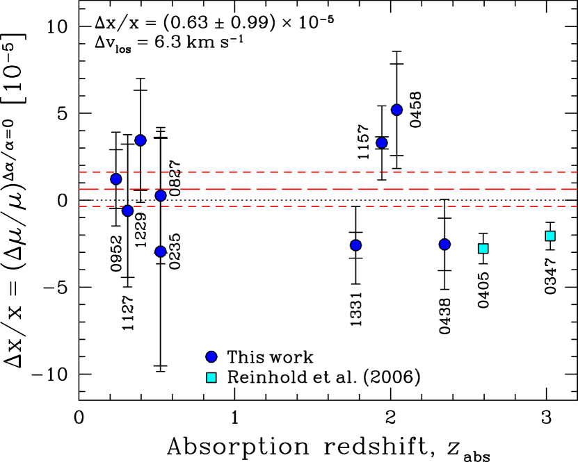
Figure 1: $\Delta x/x$ results for the nine absorption systems in our quasar sample. Initial (increased) error bars have wider (narrower) error-bar terminators. Quasar names are given truncated to four digits. Each point represents $\langle\Delta x/x\rangle_{\rm abs}$ obtained from $z_{\rm 21}$ and $\langle z_{\rm UV}\rangle$, for all heavy element species in the UV quasar spectrum, versus average $\langle z_{\rm UV}\rangle$ for that spectrum. The long-dashed horizontal line is result 3 and the short-dashed lines show the $\pm 1\sigma$ range. Under the assumption of $\Delta\alpha/\alpha$ $=0$ our results translate to constraints on $\Delta\mu/\mu$ and can be compared with the direct constraints from two H₂-bearing absorbers in Reinhold et al. (2006).

3.3.3 Method 3

For result 2, the $\chi^{2}$ per degree of freedom, $\nu$, about the weighted mean is $\chi^{2}/\nu$ $\sim 8$, well beyond what is expected based on the size of the individual error bars (i.e. $\chi^{2}/\nu$ $\sim 1$). Given the difficulty in associating 21-cm and UV velocity components, this provides motivation to quantify this additional scatter by increasing the individual uncertainties on $\langle\Delta x/x\rangle_{\rm abs}$ by an amount $s$ so as to force $\chi^{2}/\nu$ to unity. That is, the total uncertainty for each absorber is given by

$$(\sigma_{\langle\Delta x/x\rangle_{\rm abs}}^{2}+s^{2})^{0.5}.$$ (5)

A value of $\chi^{2}/\nu$ $=1$ is achieved when $s=2.10\times 10^{-5}$. The error bars now include the statistical uncertainties (as in result 2) and a systematic component which stems from the problem of comparing 21-cm and UV profiles. With these increased error bars, the weighted mean result is now $\langle\Delta x/x\rangle^{\rm weighted}_{\rm total}$ $=(0.63\pm 0.99)\times 10^{-5}$ which we label ‘result 3’. The increased uncertainty for each absorption system is shown with narrower error-bar terminators in Fig. 1. We argue below that this new error reflects much better the inherent uncertainty in the determination of $\Delta x/x$ and, as a by-product, it provides the first reliable estimate for the line-of-sight velocity differences between 21-cm and UV absorption. We treat this is our main result.

Table 2: $\Delta x/x$ result summary. Column 1 gives the label used for the method and result. Column 2 is a brief description of the error determination method. Column 3 mentions the type of $\Delta x/x$ total result. Column 4 gives the actual result. Result 3 is our fiducial constraint on $\Delta x/x$.

Label	Error type	$\Delta x/x$ type	Result [$10^{-5}$]
1	Standard error	$\langle\Delta x/x\rangle_{\rm total}$	$0.52\pm 0.99$
	on the mean
2	Formal statistical	$\langle\Delta x/x\rangle^{\rm weighted}_{\rm total}$	$1.99\pm 0.30$
	propagation
3	Increased error-bars	$\langle\Delta x/x\rangle^{\rm weighted}_{\rm total}$	$0.63\pm 0.99$

3.3.4 Variation in $x$ with cosmic time

Using the increased error bars above, we performed a linear least squares fit, $\langle\Delta x/x\rangle_{\rm abs}$ $=-\dot{x}/x\,\langle t_{\rm lb}\rangle_{\rm abs}$, where $\langle t_{\rm lb}\rangle_{\rm abs}$ is the average look-back time calculated from the $\langle z_{\rm UV}\rangle$ values in an absorption system. The best fit gives $\dot{x}/x=(-0.6\pm 1.2)\times 10^{-15}{\rm\,yr}^{-1}$. Note that by choosing this fitting function, the intercept of which is zero, we implicitly assume that $\Delta x/x=0$ at $z=0$. Although this may be corroborated by terrestrial experiments, it has not been checked in other locations corresponding to $z=0$ with the same technique used here (e.g. using 21-cm/UV absorbers elsewhere in our own galaxy).

3.3.5 Angular variation in $x$ across the sky

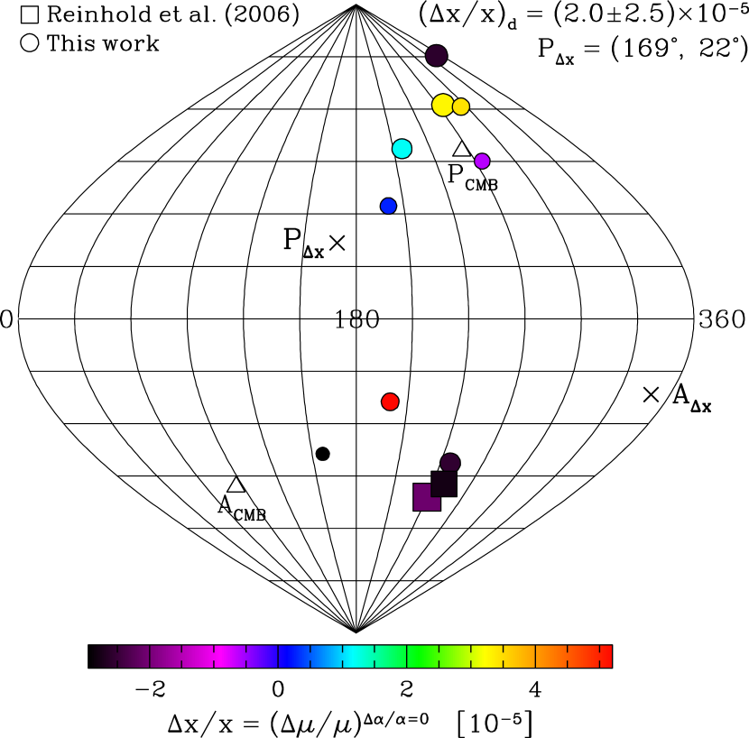
Figure 2: $\Delta x/x$ results for our nine absorbers plotted over the sky in Galactic coordinates. The grey- or colour-scale encodes the $\langle\Delta x/x\rangle_{\rm abs}$ values shown in Fig. 1 with increased error-bars. The size of the data points scale with the inverse error-bar. The pole ($P_{\Delta x}$) and anti-pole ($A_{\Delta x}$) of the best-fit dipole variation in $x$ is marked and the amplitude of the dipole is given. It is not statistically significant. The CMB pole and anti-pole are marked for comparison. Assuming $\Delta\alpha/\alpha$ $=0$, our results constrain $\Delta\mu/\mu$ and can be compared with the more direct constraints on $\Delta\mu/\mu$ by Reinhold et al. (2006). Including these additional points, the pole moves to $P_{\Delta\mu}=(190^{\circ},35^{\circ})$ and the amplitude becomes $(\Delta\mu/\mu)_{\rm d}=(4.9\pm 1.7)\times 10^{-5}$, which is formally significant. However, the dipole model is only preferred over the constant/monopole model at the 1.6-$\sigma$ level (see text).

If very large scale ($\sim$10 Gpc) spatial variations exist, one might expect $x$ to be different in different directions on the sky. We plot the distribution of $\Delta x/x$ over Galactic coordinates ($l,b$) in Fig. 2. The grey-scale indicates $\langle\Delta x/x\rangle_{\rm abs}$ and the size of each point scales with the inverse of the error on $\langle\Delta x/x\rangle_{\rm abs}$.

There is no obvious dipole (or otherwise) angular variation evident in Fig. 2. We used a $\chi^{2}$ minimisation algorithm to find the best-fit dipole in the angular distribution of $\Delta x/x$. A grid of directions in equatorial coordinates, (RA, DEC), was constructed and for each direction, a cosine fit to $\Delta x/x$ as a function of the angular distance, $\phi$, to each absorption system is performed. This yields an amplitude for the dipole, $($$\Delta x/x$$)_{\rm d}$, defined by

$$\Delta x/x(\phi)=\left<\Delta x/x\right>^{\rm weighted}_{\rm total}+\left(\Delta x/x\right)_{\rm d}\cos{\phi}\,.$$ (6)

The best-fit dipole has an amplitude $(\Delta x/x)_{\rm d}=(2.0\pm 2.5)\times 10^{-5}$ and is in the direction $P_{\Delta x}({\rm RA},\rm{\rm DEC})=(7.0{\rm\,hr},48^{\circ})$ or $P_{\Delta x}(l,b)=(169^{\circ},22^{\circ})$ as marked on Fig. 2. The dipole is not significant, despite the fact that we identified the best-fit direction (see further discussion below).

3.4 $\Delta\mu/\mu$ results

Results on $\Delta x/x$ can be used directly to obtain limits on the variation of $\mu$. From the definition of $x$ we obtain

$$\frac{\mu_{z}-\mu_{0}}{\mu_{0}}\equiv\Delta\mu/\mu=\Delta x/x-2\Delta\alpha/\alpha-\Delta g_{\rm p}/g_{\rm p}\ .$$ (7)

Furthermore, the dependence of $g_{\rm p}$ on fundamental constants is fairly weak: $\Delta g_{\rm p}/g_{\rm p}\approx-0.1\frac{\Delta(m_{q}/\Lambda_{\rm QCD})}{(m_{q}/\Lambda_{\rm QCD})}$ (Flambaum et al., 2004), where $\Lambda_{\rm QCD}$ is the quantum chromodynamic scale. Therefore the $g_{\rm p}$ term in Equation 7 can be neglected, so that there is a simple relation between $\Delta\mu/\mu$, $\Delta x/x$ and $\Delta\alpha/\alpha$. Note that relations between the variation of $\alpha$, fundamental masses and $\Lambda_{\rm QCD}$ based on Grand Unification Theories are discussed, e.g., by Marciano (1984); Calmet & Fritzsch (2002); Langacker et al. (2002); Olive et al. (2002); Dent & Fairbairn (2003); Dine et al. (2003) and references therein. Within these models the variation of $\alpha$ is $1-2$ orders of magnitude smaller than the variation of fundamental masses and $\Lambda_{\rm QCD}$, so it may be neglected in the variation of $x$. However, these relations between the variations of different fundamental constants are strongly model-dependent.

Combining our result 3 for $\Delta x/x$ with the claimed detection of variations in $\alpha$ from Murphy et al. (2003) gives $\Delta\mu/\mu=(1.7\pm 1.0)\times 10^{-5}$. In this case, the non-zero $\Delta\alpha/\alpha$ drives the resulting non-zero $\Delta\mu/\mu$. Using the claimed null-result on $\Delta\alpha/\alpha$ of Chand et al. (2004) yields $\Delta\mu/\mu=(0.75\pm 1.0)\times 10^{-5}$. Although these two varying-$\alpha$ results are quite different, note that the error-bar in the resulting value of $\Delta\mu/\mu$ is completely dominated by the error in $\Delta x/x$. Alternatively, by conservatively assuming $\Delta\alpha/\alpha$ $=0$, we obtain $\Delta\mu/\mu$ $=$ $\langle\Delta x/x\rangle^{\rm weighted}_{\rm total}$ $=(0.63\pm 0.99)\times 10^{-5}$.

Note that the dependence of the proton mass on the current quark mass, $m_{q}$, is very weak ($\Delta m_{p}/m_{p}\approx 0.05\Delta m_{q}/m_{q}$, Flambaum et al., 2004). To high accuracy the proton mass is proportional to the strong interaction parameter $\Lambda_{\rm QCD}$. Therefore, the limit on $\mu\equiv m_{\rm e}/m_{\rm p}$ is simultaneously a limit on the more fundamental Standard Model parameter $\nu\equiv m_{\rm e}/\Lambda_{\rm QCD}$ since $\Delta\mu/\mu\approx\Delta\nu/\nu$.

3.4.1 Variation in $\mu$ at high-redshift

Reinhold et al. (2006) used two H₂-bearing absorbers, one at $z_{\rm abs}=2.594$ towards Q0405$-$443 and the other at $z_{\rm abs}=3.025$ towards Q0347$-$383, to derive $\Delta\mu/\mu$ $=(-2.78\pm 0.88)$ and $(-2.06\pm 0.79)\times 10^{-5}$, respectively, (formally) indicating a significant detection of cosmological variations in $\mu$. Their quoted mean result is $(-2.4\pm 0.6)\times 10^{-5}$ (weighted fit) and $(-2.0\pm 0.6)\times 10^{-5}$ (unweighted fit). Taken at face value, the error-bar on $\Delta\mu/\mu$ from our results is comparable with the precision of these latest direct constraints on $\Delta\mu/\mu$. In that case, even assuming that $\Delta\alpha/\alpha$ $=0$ at high redshift, our null result 3 on $\langle\Delta x/x\rangle^{\rm weighted}_{\rm total}$ appears to contrast sharply with these more direct measurements of $\Delta\mu/\mu$.

The Reinhold et al. data are plotted in Fig. 1 for comparison with our constraints on $\Delta x/x$. If the apparent discrepancy between these two data-sets is to be resolved by appealing to time-variations in $\mu$, then clearly very sharp and possibly oscillatory variations would be required. However, our full data set shows a significant gap in redshift, $\Delta z\sim 1.25$. This naturally divides our set into a low- and a high-redshift subset. As the two Reinhold et al. datapoints are at high redshift, it is clear that they are best compared with our subset of four high-redshift points, the results for which are shown in Table 3. As can be seen in this table, apart from the case of pure statistical propagation of errors, our results have a factor of $\sim 2$ lower precision than those of Reinhold et al., and, given the uncertainties, are, in fact, in agreement ($2\sigma$).

Table 3: $\Delta\mu/\mu$ result summary. These results were produced in the same way as those tabulated in Table 2 but only the four highest-redshift absorbers have been used. Rows 1, 2 and 3a are for $\Delta\alpha/\alpha$ $=0$, row 3b for $\Delta\alpha/\alpha$ from Murphy et al. (2003) and row 3c for $\Delta\alpha/\alpha$ from Chand et al. (2004).

Label	Error type	$\Delta\mu/\mu$ type	Result [$10^{-5}$]
1	Standard error	$\langle\Delta\mu/\mu\rangle_{\rm total}$	$0.84\pm 2.00$ 1
	on the mean
2	Formal statistical	$\langle\Delta\mu/\mu\rangle^{\rm weighted}_{\rm total}$	$2.04\pm 0.31$ 1
	propagation
3a	Increased error-bars	$\langle\Delta\mu/\mu\rangle^{\rm weighted}_{\rm total}$	$0.58\pm 1.95$ 1
3b			$1.73\pm 1.96$ 2
3c			$0.70\pm 1.95$ 3

1:$\Delta\alpha/\alpha$ $=0$; 2:$\Delta\alpha/\alpha$ from Murphy et al. (2003); 3:$\Delta\alpha/\alpha$ from Chand et al. (2004)

3.4.2 Variation in $\mu$ with cosmic time

Using a similar approach to that for $\dot{x}/x$ above, we assume a linear variation of $\mu$ with time to constrain $\dot{\mu}/\mu$. With the increased error bars on the $\langle\Delta x/x\rangle_{\rm abs}$ values, assuming $\Delta\alpha/\alpha$ $=0$ and including the results of Reinhold et al. (2006), the time-variation of $\mu$ is constrained to be $\dot{\mu}/\mu=(1.7\pm 0.5)\times 10^{-15}{\rm\,yr}^{-1}$. Again, we assume that $\Delta\mu/\mu$ $=0$ at zero redshift but, once more, we emphasize that no absorption-line checks at $z=0$ have been made to justify this assumption.

3.4.3 Angular variation in $\mu$ across the sky

Figure 2 shows the two Reinhold et al. absorbers plotted on the sky with our $\Delta\mu/\mu$ values (i.e. our $\langle\Delta x/x\rangle_{\rm abs}$ values assuming $\Delta\alpha/\alpha$ $=0$). Given the concentration of points with $\Delta\mu/\mu$ $<0$ below the Galactic equator and the mix of values above, it is tempting to explain the apparent discrepancy between these two data-sets by spatial variations in $\mu$ across the sky. We performed a similar dipole search as for $x$ above, including the Reinhold et al. data, finding the best-fit dipole direction to be $P_{\Delta\mu}({\rm RA},\rm{\rm DEC})=(8.5{\rm\,hr},33^{\circ})$ or $P_{\Delta\mu}(l,b)=(190^{\circ},35^{\circ})$. The dipole amplitude is $(\Delta\mu/\mu)_{\rm d}=(4.9\pm 1.7)\times 10^{-5}$.

However, the limited range of angular separations in Fig. 2 severely limits the dipole interpretation. Although the dipole amplitude is formally significant at the 2.9-$\sigma$ level, this is only after we had selected the best-fit direction; this does not answer the question ‘how significantly is the dipole model preferred over the constant (i.e. monopole) model?’. We address this question using a bootstrap technique. Bootstrap samples are formed by randomising the values of $\Delta\mu/\mu$ over the quasar sight-line directions and the best-fitting dipole direction and amplitude is determined for each bootstrap sample. The resulting probability distribution for $(\Delta\mu/\mu)_{\rm d}$ indicates that values at $>$2.9-$\sigma$ significance occur 12 per cent of the time by chance alone. Therefore, the data only marginally support significant angular variations in $\Delta\mu/\mu$ given the sparse coverage of the sky.

Table 4: Alternative results. The results shown in Columns 2, 3 and 4 were obtained by introducing the changes briefly described in Column 1 (see text for more details). All results shown here were obtained using method 3.

Change	$\langle\Delta x/x\rangle^{\rm weighted}_{\rm total}$$/10^{-5}$	$\Delta\mu/\mu$$/10^{-5}$(a)	$\Delta\mu/\mu$$/10^{-5}$(b)	$\Delta v_{\rm los}$
quoted result	$0.63\pm 0.99$	$1.78\pm 1.02$	$0.63\pm 0.99$	6.3 km s-1
$z_{\rm 21}$ from literature	$0.97\pm 1.05$	$2.11\pm 1.07$	$0.97\pm 1.05$	6.8 km s-1
$+$ no digitised plots	$1.20\pm 1.22$	$2.35\pm 1.24$	$1.20\pm 1.22$	8.0 km s-1
$z_{\rm 21}$ from Gaussians	$0.49\pm 0.94$	$1.64\pm 0.96$	$0.49\pm 0.94$	5.8 km s-1
with Ca ii	$0.71\pm 0.96$	$2.38\pm 0.99$	$0.71\pm 0.96$	6.1 km s-1

^a$\Delta\alpha/\alpha$ from Murphy et al. (2003); ^b$\Delta\alpha/\alpha$ $=0$.

4 Discussion

The main result of this work is that the data show no evidence for any time variation of $\Delta x/x$. It can be seen from Fig. 1 that the $\langle\Delta x/x\rangle_{\rm abs}$ points show significant scatter beyond that expected based on their statistical (i.e. original) error bars. The error in result 1 directly reflects this scatter. After taking into account individual redshift errors and propagating them statistically, we need to increase individual uncertainties so as to obtain a $\chi^{2}/\nu$ $=1$ about the weighted mean. Even so, this procedure (method 3) gives an overall error which is essentially the same as for result 1. This simply says that the scatter in $\langle\Delta x/x\rangle_{\rm abs}$ completely dominates any errors in individual redshift measurements. This is an a posteriori justification of the validity of method 1, in which individual redshift errors were neglected and not propagated statistically. The importance of this has not been realised before, as this is the first time that $\Delta x/x$ has been determined for a sample of objects. If one determined $\Delta x/x$ for a single quasar, there would be no scatter, but there would still be a hidden and unquantifiable systematic error. In practise, of course, for a sample of systems, as we have here, this additional error has random sign and magnitude and can be treated statistically. However, our result shows that any purely statistical determination of uncertainties, i.e. without taking the observed scatter into account, would inevitably underestimate the true uncertainty.

For example, Cowie & Songaila (1995) used neutral carbon lines (C i and C i^∗) observed in the Keck/HIRES absorption spectrum of Q1331$+$170, to obtain $\Delta x/x$ $=(0.70\pm 0.55_{\rm stat})\times 10^{-5}$. For the same object we obtain $\Delta x/x$ $=(-2.59\pm 0.74_{\rm stat}\pm 2.10_{\rm syst})\times 10^{-5}$. The similarity in the statistical errors demonstrates our point. Here our statistical error is just

$$\left[\frac{(\sigma_{\langle z\rangle_{\rm UV}}^{2}+\sigma_{z_{\rm 21}}^{2})}{(1+z_{\rm 21})^{2}}\right]^{0.5}\ ,$$ (8)

and the systematic error is simply the value for the additional uncertainty $s$ which gives a $\chi^{2}/\nu$ value of 1 (Section 3.3.3). We can only determine this because we have several objects. The central value of Cowie & Songaila (1995) is different because they used a $z_{\rm UV}$ value which is a weighted mean for observed components (Songaila et al., 1994) and leads to a value very close to $z_{\rm 21}$. Further explanation of the discrepancy in the central value may come from the fact that, in this system, we have used 23 distinct UV heavy element transitions with strongest components well defined within a few km s^-1.

The preponderance of the scatter over redshift uncertainties in determining the overall error also eliminates any worry about errors introduced via the digitisation process. We emphasise that having the original digital data would not have lead to appreciably different results in this work.

What does this quantified scatter, $s$, mean? Simply from looking at the 21-cm and UV absorption profiles in Figs. 3–11, it clearly means that the assumption that 21-cm and UV absorption occurs at the same physical location is not correct. In other words the 21-cm and UV absorbing gases are randomly offset in space. A rough estimate of the average line-of-sight velocity difference is given by $\Delta v_{\rm los}\sim cs=6.3$ km s^-1. We may explain this difference qualitatively. The emitting 21-cm quasar source may appear to have a large angular size to the absorber. A 21-cm sight-line can then intersect a cold, neutral hydrogen cloud with little or no heavy elements, whilst a UV/optical sight-line can intersect another cloud with heavy elements at quite a different velocity. Such a large angular size may be due to the combined effects both of physical proximity of the absorber to the quasar and of intrinsic size of the radio emitting region. An alternative explanation involving small scale motion of the interstellar medium has been suggested by Carilli et al. (2000) in the case of the $\sim 10$ km s^-1 velocity difference between 21-cm and mm absorption lines.

The robustness of our $\Delta x/x$ and $\Delta\mu/\mu$ results, as well as our estimate of $\Delta v_{\rm los}$, can be investigated by means of alternative calculations. Table 4 summarises the simple tests we have carried out. All results quoted here have been obtained by applying method 3. Firstly, if we use $z_{\rm 21}$ directly from the literature, we obtain, for $\langle\Delta x/x\rangle^{\rm weighted}_{\rm total}$, $\Delta\mu/\mu$ (with $\Delta\alpha/\alpha$ from Murphy et al., 2003) and $\Delta\mu/\mu$ (with $\Delta\alpha/\alpha$ $=0$), $0.97\pm 1.05$, $2.11\pm 1.07$ and $0.97\pm 1.05$, respectively, and in units of $10^{-5}$ (row 2 in Table 4). If, additionally, we exclude any results for Q0235$+$164 and Q1127$-$145, we obtain $1.20\pm 1.22$, $2.35\pm 1.24$ and $1.20\pm 1.22$ (row 3 in Table 4). We have also fitted Gaussians to the 21-cm absorption profiles and used these to calculate $z_{\rm 21}$, i.e. we used the location of the minimum in the fitted Gaussian profile rather than the pixel of minimum intensity. We then obtained $0.49\pm 0.94$, $1.64\pm 0.96$ and $0.49\pm 0.94$ (row 4 in Table 4). Finally, we have investigated what happens if one includes the Ca ii lines in the calculations as well. This gives $0.71\pm 0.96$, $2.38\pm 0.99$ and $0.71\pm 0.96$. Note that, because we include Ca ii, we have no problem calculating $\sigma_{\bar{w}}$ (Section 3.3.2) for quasars Q0235$+$164, Q0952$+$179 and Q0827$+$243.

It is thus obvious that our results are relatively insensitive to the method used to estimate absorption redshifts, and, perhaps, even to the ionisation level of the transitions used. The dominant factor is the scatter due to the velocity mismatch between 21-cm and UV transitions. Because the uncertainties in our determinations of UV redshifts are small when compared to this velocity mismatch, we do not expect that standard Voigt profile fitting of the UV absorption features would significantly affect our results either. The mean line-of-sight velocity differences may become comparable in magnitude to individual errors in redshift measurements only if a much larger ($\sim 100$) sample of 21 cm/UV absorbers is obtained: The average uncertainty per absorption system due to the velocity offset is now $\sim 10^{-5}$ but with 100 absorbers, or so, we would expect this to be reduced by a factor of $\sqrt{100}$, i.e. to $\sim 10^{-6}$. A definitive answer to the question of whether $\Delta x/x$ varies, or not, with cosmic time, will have to wait until then.

Another important result is that, even when we conservatively assume $\Delta\alpha/\alpha$ $=0$, our measurements of $\Delta x/x$ imply constraints on $\Delta\mu/\mu$ which are independent of the current possible detections of Reinhold et al. (2006). These authors find a combined (unweighted) value of $\Delta\mu/\mu=(-2.0\pm 0.6)\times 10^{-5}$ from two H₂-bearing absorbers while we obtain a less direct constraint of $\Delta\mu/\mu=(0.58\pm 1.95)\times 10^{-5}$. This new constraint, based on four high-redshift 21-cm/UV absorbers combined with the assumption of $\Delta\alpha/\alpha$ $=\Delta g_{\rm p}/g_{\rm p}=0$, serves as an internally robust, independent comparison to the H₂ measurements.

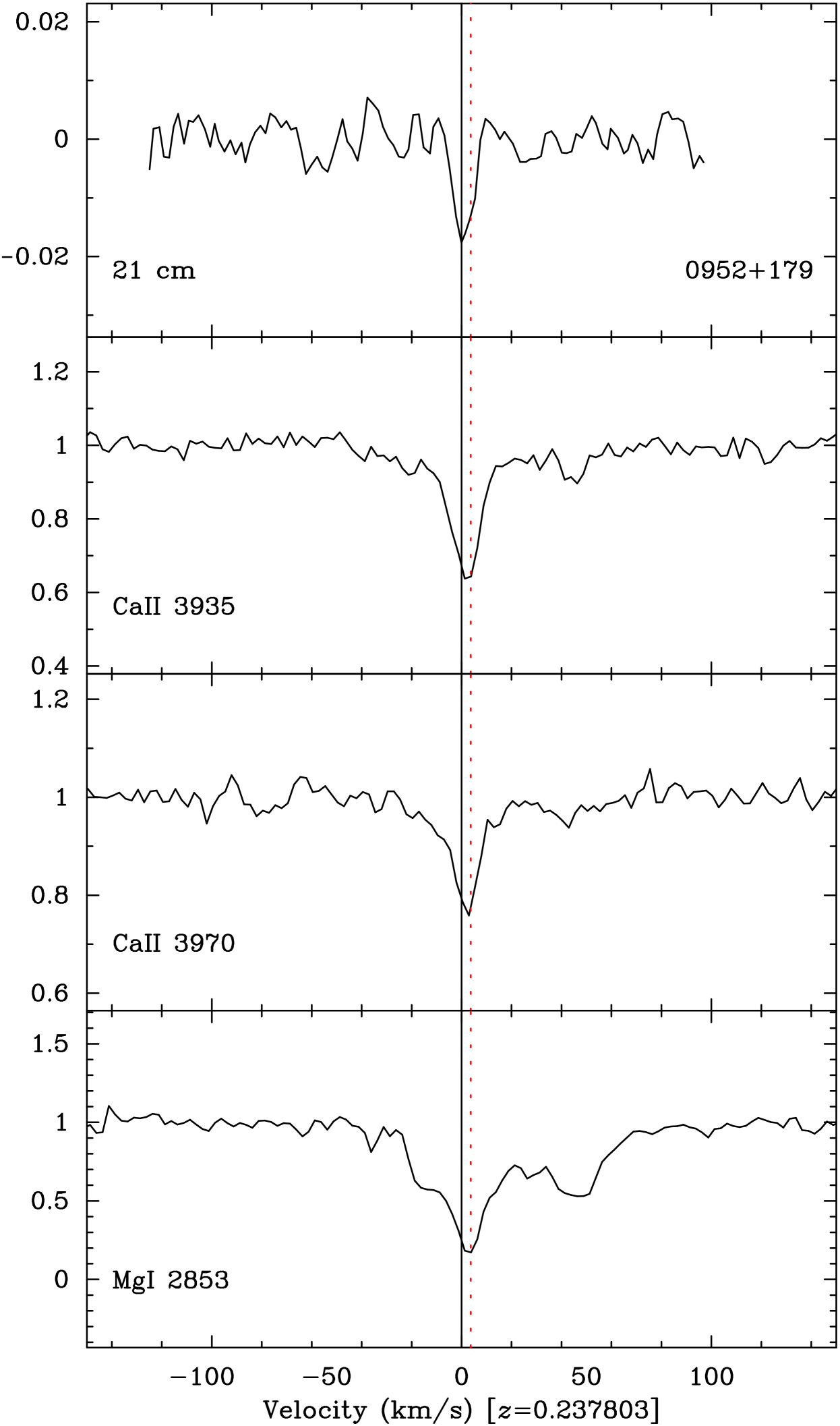
Figure 3: Velocity plot for 21-cm and UV absorption towards quasar Q0952$+$179. The 21-cm data are in units of flux (Jy). The quasar continuum (1.4 Jy) has been subtracted. The UV data are continuum normalised. The solid vertical line at 0 km s^-1 is at $z_{\rm 21}$. The dotted vertical line is at $\langle z_{\rm UV}\rangle$. In this and subsequent plots Ca ii is shown for illustration only but has not been used in the calculation of the plotted $\langle z_{\rm UV}\rangle$.

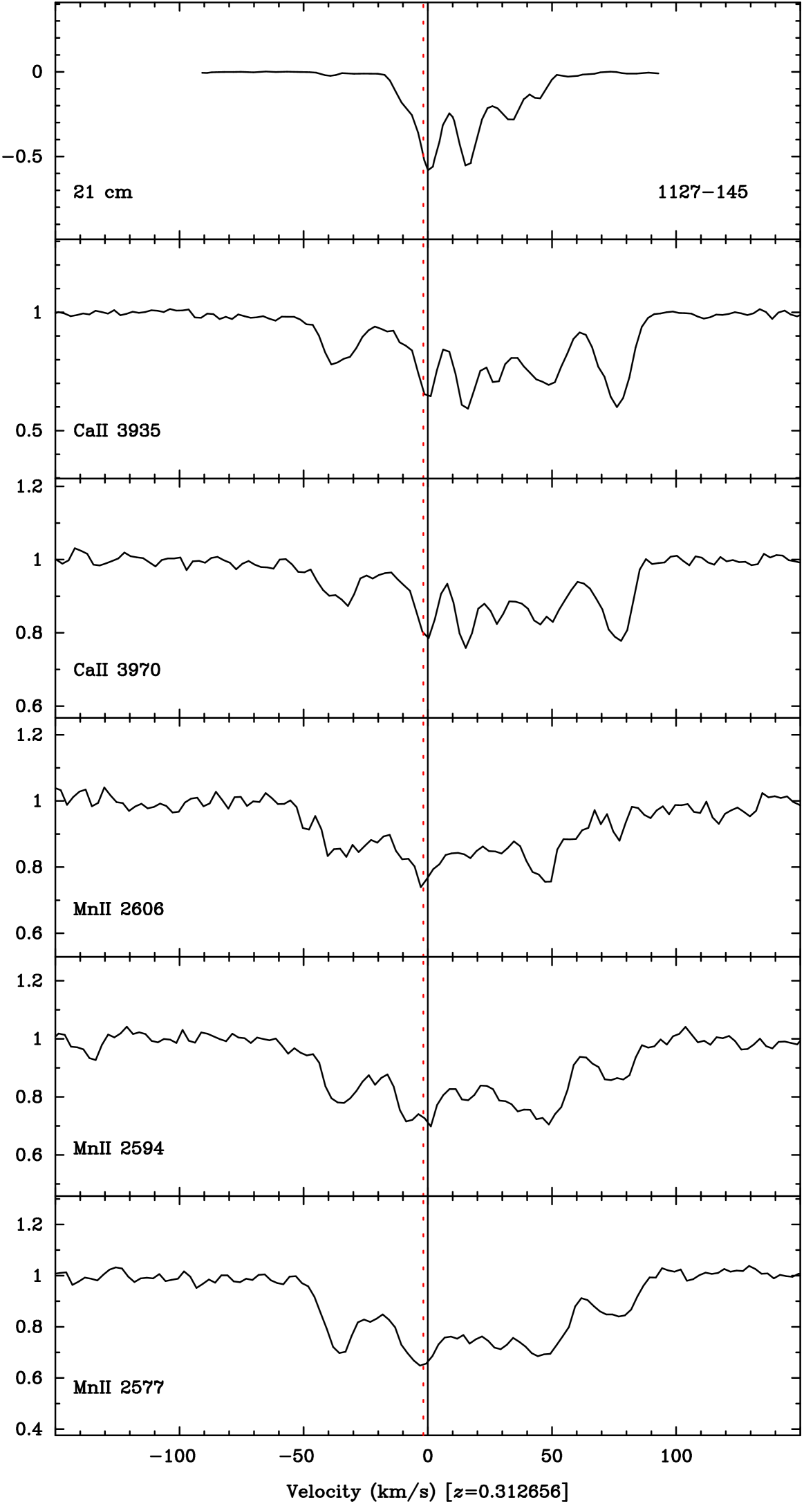
Figure 4: Velocity plot for 21-cm and UV absorption towards quasar Q1127$-$145. The 21-cm data are in units of flux (Jy). The quasar continuum (6.3 Jy) has been subtracted. The UV data are continuum normalised. The solid vertical line at 0 km s^-1 is at $z_{\rm 21}$. The dotted vertical line is at $\langle z_{\rm UV}\rangle$.

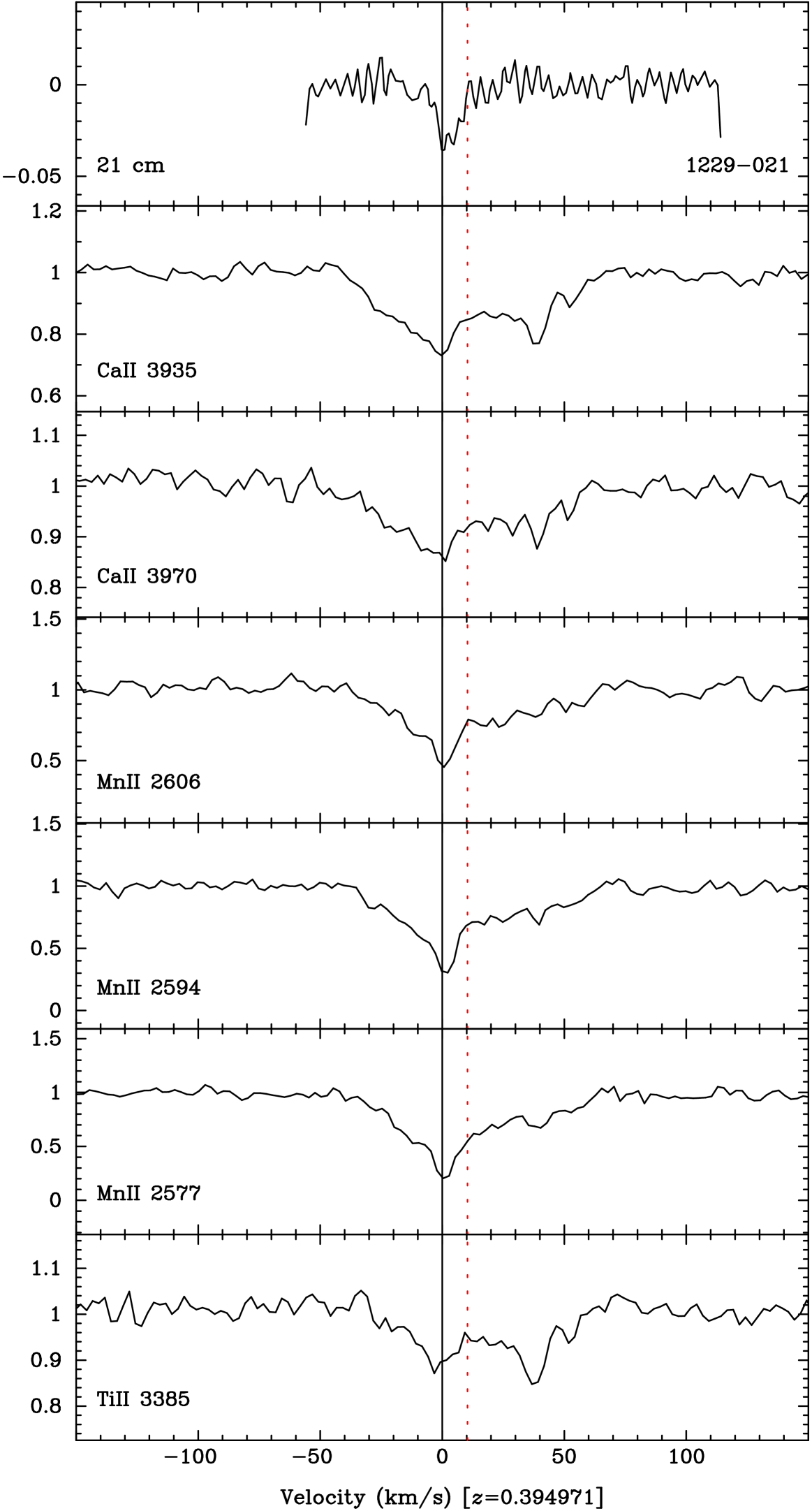
Figure 5: Velocity plot for 21-cm and UV absorption towards quasar Q1229$-$021. The 21-cm data are in units of antenna temperature (K), where the system temperature was 45 K. The UV data are continuum normalised. The solid vertical line at 0 km s^-1 is at $z_{\rm 21}$. The dotted vertical line is at $\langle z_{\rm UV}\rangle$.

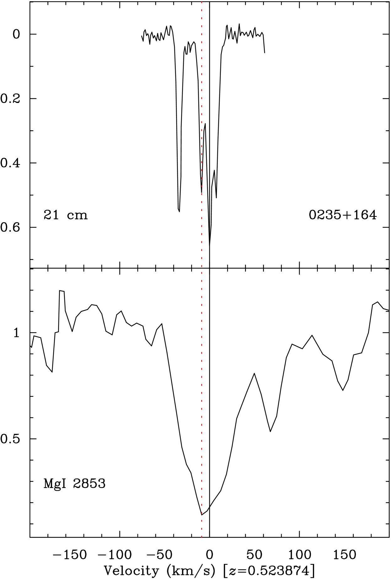
Figure 6: Velocity plot for 21-cm and UV absorption towards quasar Q0235$+$164. The 21-cm data are in units of optical depth. The UV data are continuum normalised. The solid vertical line at 0 km s^-1 is at $z_{\rm 21}$. The dotted vertical line is at $\langle z_{\rm UV}\rangle$.

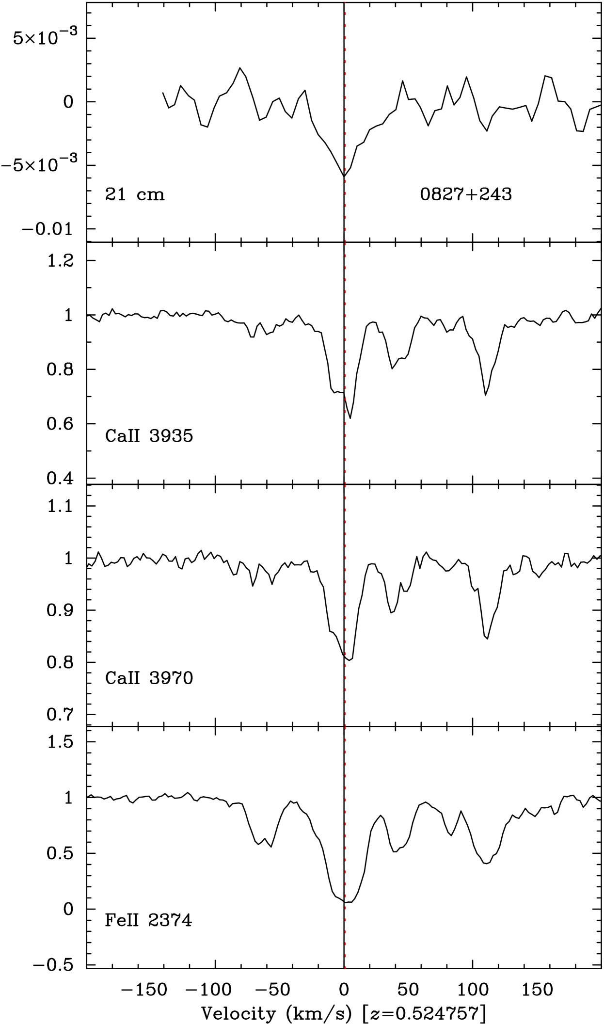
Figure 7: Velocity plot for 21-cm and UV absorption towards quasar Q0827$+$243. The 21-cm data are in units of flux (Jy) with the quasar continuum (0.9 Jy) subtracted. The UV data are continuum normalised. The solid vertical line at 0 km s^-1 is at $z_{\rm 21}$. The dotted vertical line is at $\langle z_{\rm UV}\rangle$.

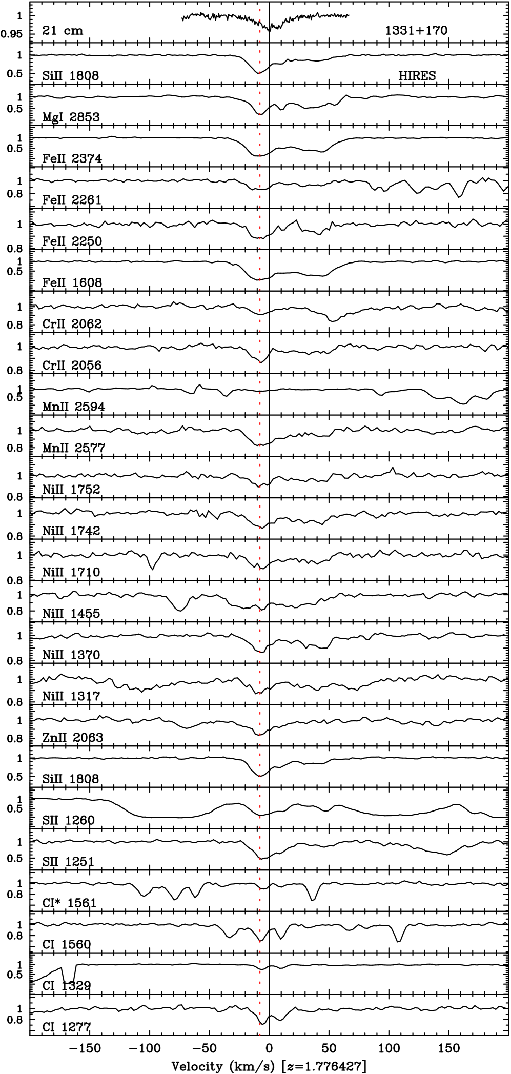
Figure 8: Velocity plot for 21-cm and UV absorption towards quasar Q1331$+$170. Both the 21-cm and UV data are continuum normalised. The solid vertical line at 0 km s^-1 is at $z_{\rm 21}$. The dotted vertical line is at $\langle z_{\rm UV}\rangle$.

References

- Avelino et al. (2001) Avelino P. P., Esposito S., Mangano G., Martins C. J. A. P., Melchiorri A., Miele G., Pisanti O., Rocha G., Viana P. T. P., 2001, Phys. Rev. D., 64, 103505
- Ballester et al. (2000) Ballester P., Modigliani A., Boitquin O., Cristiani S., Hanuschik R., Kaufer A., Wolf S., 2000, ESO Messenger, 101, 31
- Brown & Spencer (1979) Brown R. L., Spencer R. E., 1979, ApJ, 230, L1
- Calmet & Fritzsch (2002) Calmet X., Fritzsch H., 2002, Eur. Phys. J. C, 24, 639
- Carilli et al. (2000) Carilli C. L., Menten K. M., Stocke J. T., Perlman E., Vermeulen R., Briggs F., de Bruyn A. G., Conway J., Moore C. P., 2000, Phys. Rev. Lett., 85, 5511
- Chand et al. (2004) Chand H., Srianand R., Petitjean P., Aracil B., 2004, A&A, 417, 853
- Cowie & Songaila (1995) Cowie L. L., Songaila A., 1995, ApJ, 453, 596
- Curran et al. (2005) Curran S. J., Murphy M. T., Pihlström Y. M., Webb J. K., Purcell C. R., 2005, MNRAS, 356, 1509
- Demleitner et al. (2001) Demleitner M., Accomazzi A., Eichhorn G., Grant C. S., Kurtz M. J., Murray S. S., 2001, in ASP Conf. Ser. 238: Astronomical Data Analysis Software and Systems X ADS’s Dexter Data Extraction Applet. p. 321
- Dent & Fairbairn (2003) Dent T., Fairbairn M., 2003, Nuc. Phys. B, 653, 256
- Dine et al. (2003) Dine M., Nir Y., Raz G., Volansky T., 2003, Phys. Rev. D., 67, 015009
- Dmitriev et al. (2004) Dmitriev V. F., Flambaum V. V., Webb J. K., 2004, Phys. Rev. D, 69, 063506
- Dzuba et al. (1999) Dzuba V. A., Flambaum V. V., Webb J. K., 1999, Phys. Rev. Lett., 82, 888
- Flambaum et al. (2004) Flambaum V. V., Leinweber D. B., Thomas A. W., Young R. D., 2004, Phys. Rev. D, 69, 115006
- Flambaum & Shuryak (2002) Flambaum V. V., Shuryak E. V., 2002, Phys. Rev. D, 65, 103503
- Flambaum & Tedesco (2006) Flambaum V. V., Tedesco A. F., 2006, Phys. Rev. C, 73, 055501
- Foltz et al. (1988) Foltz C. B., Chaffee F. H., Black J. H., 1988, ApJ, 324, 267
- Fujii et al. (2000) Fujii Y., Iwamoto A., Fukahori T., Ohnuki T., Nakagawa M., H. H., Oura Y., Möller P., 2000, Nucl. Phys. B, 573, 377
- Ivanchik et al. (2005) Ivanchik A., Petitjean P., Varshalovich D., Aracil B., Srianand R., Chand H., Ledoux C., Boissé P., 2005, A&A, 440, 45
- Ivanchik et al. (2002) Ivanchik A. V., Rodriguez E., Petitjean P., Varshalovich D. A., 2002, Astron. Lett., 28, 423
- Kanekar & Chengalur (2001a) Kanekar N., Chengalur J. N., 2001a, A&A, 369, 42
- Kanekar & Chengalur (2001b) Kanekar N., Chengalur J. N., 2001b, MNRAS, 325, 631
- Kanekar et al. (2006) Kanekar N., Subrahmanyan R., Ellison S. L., Lane W. M., Chengalur J. N., 2006, MNRAS, 370, L46
- Karshenboim et al. (2005) Karshenboim S. G., Flambaum V. V., Peik E., 2005, Handbook of Atomic, Molecular and Optical Physics. Springer, Berlin, p. 459
- Lamoreaux & Torgerson (2004) Lamoreaux S. K., Torgerson J. R., 2004, Phys. Rev. D, 69, 121701
- Landau et al. (2001) Landau S., Harari D., Zaldarriaga M., 2001, Phys. Rev. D, 63, 083505
- Langacker et al. (2002) Langacker P., Segrè G., Strassler M. J., 2002, Phys. Lett. B, 528, 121
- Lanzetta & Bowen (1992) Lanzetta K. M., Bowen D. V., 1992, ApJ, 391, 48
- Levshakov & Varshalovich (1985) Levshakov S. A., Varshalovich D. A., 1985, MNRAS, 212, 517
- Marciano (1984) Marciano W. M., 1984, Phys. Rev. Lett., 52, 489
- Marion et al. (2003) Marion H., Pereira Dos Santos F., Abgrall M., Zhang S., Sortais Y., Bize S., Maksimovic I., Calonico D., Grünert J., Mandache C., Lemonde P., Santarelli G., Laurent P., Clairon A., 2003, Phys. Rev. Lett., 90, 150801
- Martins et al. (2002) Martins C., Melchiorri A., Trotta R., Bean R., Rocha G., Avelino P., Viana P., 2002, Phys. Rev. D, 66, 023505
- Meyer (1992) Meyer S. L., 1992, Data Analysis for Scientists and Engineers. John Wiley and Sons
- Murphy et al. (2004) Murphy M. T., Flambaum V. V., Webb J. K., et al. 2004, Lecture Notes in Physics Vol. 648: Astrophysics, Clocks and Fundamental Constants, 648, 131
- Murphy et al. (2003) Murphy M. T., Webb J. K., Flambaum V. V., 2003, MNRAS, 345, 609
- Murphy et al. (2001) Murphy M. T., Webb J. K., Flambaum V. V., Churchill C. W., Prochaska J. X., 2001, MNRAS, 327, 1223
- Murphy et al. (2003) Murphy M. T., Webb J. K., Flambaum V. V., Curran S. J., 2003, Ap&SS, 283, 577
- Murphy et al. (2001) Murphy M. T., Webb J. K., Flambaum V. V., Dzuba V. A., Churchill C. W., Prochaska J. X., Barrow J. D., Wolfe A. M., 2001, MNRAS, 327, 1208
- Olive et al. (2002) Olive K. A., Pospelov M., Qian Y.-Z., Coc A., Cassé M., Vangioni-Flam E., 2002, Phys. Rev. D, 66, 045022
- Prestage et al. (1995) Prestage J. D., Tjoelker R. L., Maleki L., 1995, Phys. Rev. Lett., 74, 3511
- Prochaska (2003) Prochaska J. X., 2003, ApJ, 582, 49
- Reinhold et al. (2006) Reinhold E., Buning R., Hollenstein R., Ivanchik A., Petitjean P., 2006, Phys. Rev. Lett., 96, 151101
- Shlyakhter (1976) Shlyakhter A. I., 1976, Nature, 264, 340
- Songaila et al. (1994) Songaila A., Cowie L. L., Vogt S., Keane M., Wolfe A. M., Hu E. M., Oren A. L., Tytler D. R., Lanzetta K. M., 1994, Nature, 371, 43
- Sortais et al. (2001) Sortais Y., Bize S., Abgrall M., 2001, Phys. Scr., 95, 50
- Srianand et al. (2004) Srianand R., Chand H., Petitjean P., Aracil B., 2004, Phys. Rev. Lett., 92, 121302
- Thompson (1975) Thompson R. I., 1975, Astrophys. Lett., 16, 3
- Tubbs & Wolfe (1980) Tubbs A. D., Wolfe A. M., 1980, ApJ, 236, L105
- Tzanavaris et al. (2005) Tzanavaris P., Webb J. K., Murphy M. T., Flambaum V. V., Curran S. J., 2005, Physical Review Letters, 95, 041301
- Ubachs & Reinhold (2004) Ubachs W., Reinhold E., 2004, Phys. Rev. Lett., 92, 101302
- Uzan (2003) Uzan J.-P., 2003, Rev. Mod. Phys., 75, 403
- Varshalovich & Levshakov (1993) Varshalovich D. A., Levshakov S. A., 1993, J. Exp. Theor. Phys. Lett., 58, 237
- Webb et al. (1999) Webb J. K., Flambaum V. V., Churchill C. W., Drinkwater M. J., Barrow J. D., 1999, Phys. Rev. Lett., 82, 884
- Webb et al. (2003) Webb J. K., Murphy M. T., Flambaum V. V., Curran S. J., 2003, Ap&SS, 283, 565
- Webb et al. (2001) Webb J. K., Murphy M. T., Flambaum V. V., Dzuba V. A., Barrow J. D., Churchill C. W., Prochaska J. X., Wolfe A. M., 2001, Phys. Rev. Lett., 87, 091301
- Wolfe et al. (1981) Wolfe A. M., Briggs F. H., Jauncey D. L., 1981, ApJ, 248, 460
- Wolfe et al. (1985) Wolfe A. M., Briggs F. H., Turnshek D. A., Davis M. M., Smith H. E., Cohen R. D., 1985, ApJ, 294, L67
- Wolfe et al. (1978) Wolfe A. M., Broderick J. J., Johnston K. J., Condon J. J., 1978, ApJ, 222, 752
- Wolfe & Davis (1979) Wolfe A. M., Davis M. M., 1979, AJ, 84, 699