A potentially pure test of cosmic geometry: galaxy clusters and the real space Alcock-Paczyński test

Abstract

We investigate the possibility of probing dark energy by measuring the isotropy of the galaxy cluster autocorrelation function (an Alcock-Paczyński test). The correlation function is distorted in redshift space because of the cluster peculiar velocities, but if these are known and can be subtracted, the correlation function measurement becomes in principle a pure test of cosmic geometry. Galaxy cluster peculiar velocities can be measured using the kinetic Sunyaev Zel’dovich (kSZ) effect. Upcoming CMB surveys, e.g., ACT, SPT, Planck, are expected to do this with varying levels of accuracy, dependent on systematic errors due to cluster temperature measurements, radio point sources, and the primary CMB anisotropy. We use the Hubble volume $N$-body simulation and the hydrodynamic simulation results of Nagai et. al (2003) to simulate various kSZ surveys. We find by model fitting that a measurement of the correlation function distortion can be used to recover the cosmological parameters that have been used to generate the simulation. However, the low space density of galaxy clusters requires larger surveys than are taking place at present to place tight constraints on cosmology. For example, with the SPT and ACT surveys, $\Omega_{\Lambda}$ could be measured to within 0.1 and 0.2 respectively at one sigma, but only upper limits on the equation of state parameter $w$ will be possible. Nevertheless, with accurate measurements of the kSZ effect, this test can eventually be used to probe the dark energy equation of state and its evolution with redshift, with different systematic errors than other methods.

1 Introduction

The Alcock-Paczyński (1979, hereafter AP) test is a conceptually simple probe of cosmic geometry and hence dark energy. It is based on the fact that an intrinsically isotropic object will appear distorted when we translate it from observed space (angles and redshifts) into real space (units of length) if we use the wrong cosmology (to relate angles and redshift to sizes). The strength of the distortion will depend on cosmic geometry, for example the value of the cosmological constant $\Lambda$. The test is a way to measure dark energy which requires only that we find and measure known perfectly symmetric objects in the Universe. In the present work we use the autocorrelation function of galaxy clusters as the “isotropic” object. In addition to the possible geometric distortions, the correlation function will have a distortion of different kind, which is due to peculiar velocities of clusters. This affects the line of sight component of cluster pair separations (e.g., as applied to galaxies by Davis and Peebles 1983, Kaiser 1987, and clusters by the Padilla & Baugh 2002). There is a way to remove this distortion however, by making use of the kinetic Sunyaev-Zeldovich (kSZ) effect (Sunyaev & Zeldovich 1972). The kSZ effect is the Doppler shift of CMB photons due to a hot intracluster medium. The CMB photons interact with free electrons and become Doppler shifted when the cluster is moving with respect to the CMB rest frame. This causes temperature fluctuations that depend on the bulk velocity of cluster. There are currently on-going and future surveys that plan to measure this effect (see e.g., Vale and White 2005 for strategies). At the time of writing, the kSZ effect has not yet been detected for single clusters, although upper limits on have been estimated on the bulk velocity averaged over several clusters (e.g., 1420 ${\rm\;km\;s^{-1}}$ at 95 $\%$ confidence by Benson et al. 2003). In the present paper we investigate the correction of redshift distortions from peculiar velocities using kSZ measurements, and how this can leave the pure geometric distortions from which we can find cosmological parameters.

Similar methods have been put forward for constraining cosmology with the clustering of different objects. Phillipps (1994) suggested using quasar clustering for the Alcock Paczyński test (averaging over many close pairs of quasars). Several other studies have adopted the quasar correlation function as the isotropic object (e.g., Popowski et al. 1998, Hoyle et al. 2002, da Ângela et al. 2005). The difficulty of this method is that we only observe the positions of quasars in redshift space, where the correlation function is distorted by peculiar velocities (e.g., Kaiser 1987, Hamilton 1992) and by other source of noise, such redshift errors.

Many studies have suggested using the kinetic Sunyaev-Zel’dovich effect (e.g., Haehnelt & Tegmark 1996, Lange et al. 1998, Kashilinsky & Atrio-Barandela 2000, Aghanim et al. 2001, Atrio-Barandela et al. 2004, etc.) to measure peculiar velocities of galaxy clusters. There are several upcoming sky surveys that aim to do this, such as ACT, SPT and Planck In principle, these types of measurements can be used to eliminate the distortion due to peculiar velocities and therefore we can recover the isotropic correlation function. The bulk cluster peculiar velocity is not the sole factor in the distortion and there are sources of noise in kSZ measurements. These include microwave background fluctuations, cluster internal velocities, and point source contamination (see simulations by Haehnelt & Tegmark 1996, Aghanim et al. 2005.)

In the present work, we use large N-body simulations (the Hubble volume, Evrard et al. 2002), and the hydrodynamic simulation results of Nagai et al. (2003) to test how well the peculiar velocity-corrected galaxy cluster AP test can be carried out. Our plan for the paper is as follows: In §2 we discuss the theoretical cluster correlation function we use as a model as well as that measured from the Hubble volume simulation. In §3.1, we explain the model fitting procedure and predict the effect of kSZ measurements. We describe and measure the geometric distortions as a function of redshift. Using the recovered values we constrain cosmological parameters from the simulation data, discussing the results in the same section. We show results from simulations of particular surveys (SPT and ACT) in §4.1-§4.2. We summarize our results and conclude in §5.

2 Cluster Correlation Function

The cluster autocorrelation function $\xi(r)$ is a measure of the probability of finding a cluster at a distance $r$ from another cluster; typically it is computed as the ratio of the number of clusters at a distance $r$ from another cluster [$DD(r)$], divided by the number expected in the absence of clustering [$DR(r)$] minus 1, i.e. $\xi(r)=\frac{DD(r)}{DR(r)}-1$, where DD represent cluster-cluster pairs and DR cluster-random pairs. $\xi(\sigma,\pi)$ carries the same definition but the distance between two clusters is represented in terms of the component directions perpendicular ($\sigma$) and parallel to the line of sight ($\pi$). Many groups have studied clustering of galaxies, clusters and QSOs or the cross-correlation of one with another using simulations and observations (e.g., Mo & White 1996, Mo et al. 1996, Borgani et al. 1997, Croft et al. 1999, Colberg et al. 2000, Moscardini et al. , 2000, Zehavi et al. 2002, Hawkins et al. 2003, Croom et al. , 2005, Springel et al. , 2005). Springel et al. (2005) compare the galaxy 2 point correlation function from their high-resolution simulation with that of galaxies in the 2dF, SDSS and APM surveys and show that the correlation functions follow power laws for $r<\sim 20\;h^{-1}{\rm Mpc}$ and that observation and simulation agree very well.

In the most recent Sloan Digital Sky Survey (SDSS) analysis, Zehavi et al. (2005) studied the luminosity and color dependence of the galaxy correlation function. It was found that clustering of blue galaxies increases continuously with luminosity, whereas bright red galaxies show strong clustering at large scales and faint ones mainly cluster at small scales. Many of the studies described fit the correlation function with a single power-law although this simple form was found be some not to be good enough to use (e.g., in analysis of the 2dF data by Hawkins et al. 2003, Croom et al. , 2005, da Ângela et al. 2005). These considerations will affect our choice of model correlation function, described below.

2.1 Theory

Alcock & Paczyński (1979) showed that the ratio of angular and redshift sizes of a spherical comoving object evolve differently in time for different cosmologies. Detailed discussions of how the components evolve in redshift are presented in Ballinger et al. (1996) and Matsubara and Suto (1996).

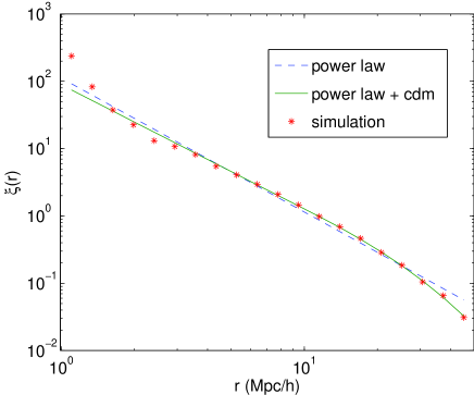
Da Ângela et al. (2005) argued that the correlation function (of high-z galaxies) cannot be described adequately with a single power law, and use a double power law when they fit it. We adopt this general idea when we build our model correlation function but instead of using two power laws, we use a single power-law for $r\leq r_{0}$ and use a correlation function computed using cold dark matter linear theory (the transfer function from Bardeen et al. 1986) for $r>r_{0}$. We test this idea using the $\Lambda$CDM Hubble volume simulation (see §2.2 for more detailed description.) Figure 1 shows the best-fit power law and the best-fit composite power-law and CDM correlation functions. It demonstrates that the latter describes the correlation function better, especially for large $r$ where the $\xi(r)$ decreases faster than a power law.

A power law correlation function is given by:

$$\xi(r)=\left(\frac{r}{r_{0}}\right)^{-\gamma}.$$ (1)

$r$ can be rewritten in terms of line of sight and transverse components,

$$r^{2} = \sigma^{2}+\pi^{2}$$ (2)

$$= f^{2}\Delta\theta^{2}+g^{2}\Delta z^{2}$$

where $f$ and $g$ are given by

$$f=(1+z)D_{A}(z),$$ (3)

and

$$g=\frac{c}{H(z)}.$$ (4)

In order to incorporate the equation of state of dark energy, we use (Seo & Eisenstein 2003)

$$H(z)=H_{0}\sqrt{\Omega_{m}(1+z)^{3}+\Omega_{X}\exp\left[3\int_{0}^{z}\frac{1+w(z)}{1+z}dz\right]}$$ (5)

and

$$D_{A}(z)=\frac{c}{1+z}\int_{0}^{z}\frac{dz}{H(z)}.$$ (6)

In our study, we assume a flat universe such that $\Omega_{m}+\Omega_{X}=1$ and allow a redshift dependent equation of state with the simple form. $w=w_{0}+w_{1}z$ (e.g., Seo & Eisenstein 2003). We introduce a distortion parameter $h$ (Popowski et al. 1998) such that

$$h\equiv\frac{1}{z}\times\frac{f}{g}.$$ (7)

With respect to a particular reference cosmology, this becomes

$$h=\frac{f/g}{f_{0}/g_{0}}.$$ (8)

To compute $f_{0}$ and $g_{0}$ we use as a reference cosmology the same cosmology used in the Hubble volume simulation ($\Omega_{m}=0.3,\Omega_{\Lambda}=0.7$). Throughout the paper we use this $h$ as the distortion parameter unless noted otherwise. Note that $\frac{\sigma}{\pi}$/$\frac{\sigma_{0}}{\pi_{0}}=\frac{f}{g}$/$\frac{f_{0}}{g_{0}}$ because $\Delta\theta$ and $\Delta z$ represent the observed quantities and are invariant with cosmology. Therefore, $h$ is defined in such a way that when $h$ is greater (less) than 1, the correlation function is stretched in the transverse (line of sight) direction.

For a given power-law correlation function used for $r\leq r_{0}$, we adjust the amplitude of the CDM correlation function so that it joins the power law exactly at $r=r_{0}$. An alternative would be to keep the amplitude of the CDM correlation function fixed but rescale $r$ so that it joins the power law. This is equivalent to assuming a different value of $\Omega h$. We briefly describe an analysis in §3 where this was done in order to test whether a better fit to the non-linear correlation function could be achieved. In our fiducial analysis, however we restrict ourselves to only changing the amplitude of the CDM $\xi$. We note that as $r_{0}$ determines the change in the amplitude, using the CDM shape does not increase the number of free parameters in the fit.

In redshift space, we observe a correlation function that is distorted because of peculiar velocities and other noise sources such as redshift errors. We assume that the distortion due to peculiar velocities can be removed using a measured kSZ velocity (we return to the validity of this assumption in §3.1) and we use a Gaussian function of width $\sigma_{v}$ to model the remaining distortion. The distortions only occur in the line of sight direction so the effect can incorporated into the correlation function using a convolution in $\pi$. Using the notation of Dalton et al. (1992), the distorted correlation function for $r\leq r_{0}$, can be written as:

$$\xi(\sigma,\pi)_{r\leq r_{0}}=\frac{r_{0}^{-\gamma}}{\sqrt{{2\pi}}\sigma_{v}}\int\left[\sigma^{2}+\left(\pi-\frac{w}{H}\right)^{2}\right]^{-\gamma}e^{-\frac{w^{2}}{2\sigma_{v}^{2}}}dw$$ (9)

When $r>r_{0}$, the CDM part of correlation function is convolved in the same way:

$$\xi(r)_{r>r_{0}}=\frac{1}{\sqrt{{2\pi}}\sigma_{v}}\int\xi_{\rm CDM}(r)e^{-\frac{w^{2}}{2\sigma_{v}^{2}}}dw$$ (10)

where $r=(\sigma^{2}+(\pi-\frac{w}{H})^{2})^{1/2}$.

Our aim is to vary $h$, $\gamma$, $r_{0}$ and $\sigma_{v}$ and compare our model correlation function with that measured from a simulation. This is to see if we can measure the distortion parameter $h$. Since $h$ is calculated with respect to the $\Omega_{m}=0.3,\Omega_{\Lambda}=0.7$ cosmology (Equation 8), we hope to recover $h=1$, thus showing that we can recover the cosmology that was used to generate the $\Lambda$CDM Hubble volume simulation.

Figure 1: The galaxy cluster correlation function from an octant of the Hubble volume simulation (points), as well as the best fit power law and our chosen fitting function (power law + linear CDM, see text.)

2.2 Simulations

We use a light-cone output of the $\Lambda$CDM Hubble Volume $N$-body simulation made publically available by the Virgo Consortium (Frenk et al. 2000). The output is of a model with $\Omega_{m}=0.3,\Omega_{\Lambda}=0.7,h=0.7$ and amplitude of mass fluctuations $\sigma_{8}=0.9$. The light cone data is an octant of the simulation volume in shape (and therefore covers $\pi/2$ steradian), with radius 3000 $\;h^{-1}{\rm Mpc}$. The redshift extends to $z=1.46$. We use the Virgo consortium cluster catalogue generated by using the spherical overdensity (SO) algorithm (Lacey & Cole 1994) with density threshold of 200, and a minimum particle count per cluster of 12 (Evrard et al. 2002). The mass of each particle is 2.2$\times 10^{12}\;h^{-1}{\rm M_{\odot}}$ and there are total of 802461 clusters with mass $>2.6\times 10^{13}\;h^{-1}{\rm M_{\odot}}$ in the catalogue. We take this data set to be our fiducial “simulated survey” i.e. a survey that covers a quarter of the sky, down to this mass limit.

We calculate the cluster correlation function using the following estimator:

$$\xi(r)=C\frac{N_{cc}}{N_{cr}}-1$$ (11)

where $N_{cc}$ is the number of cluster-cluster pairs and $N_{cr}$ is the number of cluster-random pairs. $C$ is the ratio of the number of clusters in a random catalogue to the number of clusters in the cluster catalogue. Our random catalogue has $C=20$. The random catalogues are made to have the same overall number density with redshift trends as the simulation data and the same survey boundaries. In order to do this, we bin the simulated clusters in redshift and use this to generate a number density profile as a function of redshift. We then randomly sample from this number density profile until we reach the correct total number of random points.

In order to measure the geometric distortion as a function of redshift, we divide the simulated universe into 11 redshift bins from $z=0.2$ to $z=1.3$. The space density of clusters declines at higher redshifts. For example, we have space densities of $3.5\times 10^{-5},6.0\times 10^{-6},3.9\times 10^{-6}$ clusters per comoving unit volume ($\;h^{-3}{\rm Mpc}^{3}$) for $z=0.2-0.3,0.7-0.8,$ and $1.2-1.3$ respectively (24723, 83441 and 58767 clusters in the bins.)

For each redshift bin, we compute $\xi(\sigma,\pi)$, in 2 $\;h^{-1}{\rm Mpc}$ intervals. In our fitting, we keep the 494 bins in $\xi(\sigma,\pi)$ which have $r<50\;h^{-1}{\rm Mpc}$. For $\chi^{2}$ fitting, we build a covariance matrix using the jack-knife method with 9 subvolumes of equal size. We only use the diagonal elements in the covariance matrix for our analysis. This approach is intermediate between using Poisson errors and a full covariance matrix. We do not do the latter because with a small number of subsamples the matrix becomes singular. Because galaxy clusters form a sparse sample, this simplification of the error bar calculation is reasonable (see e.g. Popowski and Weinberg 1998). We check on this by computing the $\chi^{2}$ per bin and comparing it to unity.

2.3 Distortion in Redshift Space

Observing clusters in redshift space means that cluster peculiar motions cause distortion in the correlation function. Matsubara & Suto (1996) modeled the redshift distortion of parallel and transverse components of the correlation function, and Padilla & Baugh (2002) studied the redshift distortions in the cluster correlation function using the Hubble volume simulation.

Peculiar velocities reflect large-scale cluster infall into overdense regions and result in the correlation function being squashed in the line of sight direction. In the linear regime, the flattening effect is typically described in terms of $\beta=\Omega^{0.6}_{m}/b$ where $b$ is the bias parameter. The geometric distortion and the peculiar velocity distortion both have roughly similar aspects, although they can be distinguished given large enough datasets or through their differing evolution with redshift (see e.g., Ballinger et al. 1996).

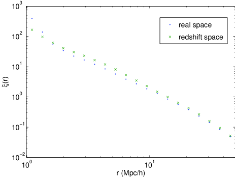
In Figure 2 we plot the correlation function as a function of $r$ in both real ($\xi_{r}$) and redshift space ($\xi_{s}$). We see the suppression of correlation function on small scales and the boost on linear scales as predicted by Kaiser (1987). The linear theory prediction is $\xi_{s}/\xi_{r}=1+\frac{2/3}{\beta}+\frac{1/5}{\beta}^{2}$, where $\beta=\Omega^{0.6}_{m}/b$, with $b$ being the bias factor for clusters. Colberg et al. (2000) reported that $b$ for these clusters is $b=2.25$, so that the linear boost correction factor due to Kaiser effect for $\Lambda$CDM is 1.150. We average over the points in the linear regime with $r>10\;h^{-1}{\rm Mpc}$ and find an average boost of 1.146, close to the linear theory prediction.

Figure 2: The simulation correlation function $\xi(r)$ for the Hubble volume octant in real and redshift space for the redshift range $z=0.8-0.9.$ The difference between the two in the linear regime agrees well with the expected Kaiser (1987) enhancement in redshift space (see text.)

Although we assume that the peculiar velocites can be removed via kSZ surveys, we still have to deal with systematic or measurement errors that can not be eliminated entirely. Unlike peculiar velocities, measurement errors will tend to stretch the correlation function along the line of sight. Padilla and Baugh (2002) showed that the cluster correlation function is not as subject as the galaxy correlation function to small scale virialized motions (“the finger of God” effect), due to the fact that superclusters are not virialized systems.

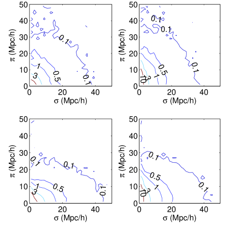
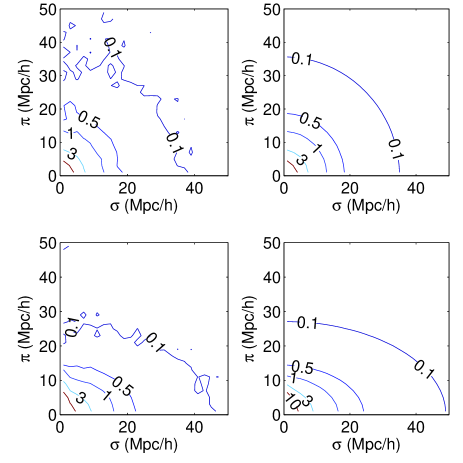
In Figure 3 we examine $\xi(\sigma,\pi)$ measured from the simulation. We show how the correlation function is distorted in redshift space when there are random errors (two right panels) and when there are peculiar velocities (two bottom panels). For the random errors, we add Gaussian redshift errors with $\sigma=400$km/s randomly to each cluster. The top left panel shows the case when there is no redshift distortion at all. The correlation function is isotropic, as expected. With random errors only, it is stretched along the line of sight (top right), and undergoes further distortion when peculiar velocities are added (bottom right). The overall squashing along the line of sight is better seen in the bottom left panel where peculiar velocities are only source of distortion (no random errors added). This agrees well with the results of Padilla & Baugh (2002) who find that there is no stretching of the correlation function due to random peculiar velocities in redshift space, but that coherent motions of clusters flatten the correlation function along the line of sight.

Nagai et al. (2003) studied the real and estimated peculiar velocities and their discrepancies with a hydrodynamical simulation. We describe their work in more detail in §2.5 below. We take their results to be representative of the minimum noise level which can be achieved in measurements of the cluster velocity.

Figure 3: Measured correlation functions from the Hubble Volume simulation for the redshift range $z=0.8-0.9$. Left (right) panels: without (with) Gaussian measurement errors of 400 $km/s$. Top (bottom) panels: without (with) peculiar velocities. The correlation function is almost isotropic when there is no redshift distortion (top left).

2.4 SZ effect

The SZ effect comprises the thermal and kinetic effects. The thermal SZ effect is a distortion of the CMB photon energy spectrum due to inverse Compton scattering in the cluster. When the CMB photons are scattered by free electrons in the hot intracluster gas, they exchange energy and the tempature decreases (increases) at low (high) frequencies, resulting in a spectral distortion skewed toward higher frequencies. The distortion due to the thermal effect (non-relativistic) is described by:

$$\frac{\Delta T_{\rm tSZ}}{T_{CMB}}=y\left(x\frac{e^{x}+1}{e^{x}-1}-4\right)$$ (12)

where $x\equiv\frac{h\nu}{k_{B}T_{CMB}}$ and

$$y=\frac{k\sigma_{T}}{m_{e}c^{2}}\int dlT_{e}(l)n_{e}\approx\tau_{e}\frac{kT_{e}}{m_{e}c^{2}}.$$ (13)

In addition, when the cluster is moving with respect to the CMB rest frame, the signal will be Doppler shifted, with an amplitude proportional to the peculiar velocity of the cluster. This is the kinetic SZ effect. The magnitude of the effect is given by

$$\frac{\Delta T_{\rm kSZ}}{T_{CMB}}=-\tau\left(\frac{v_{pec}}{c}\right)$$ (14)

where $\tau_{e}$ is the optical depth and $v_{pec}$ is the peculiar velocity component along the line of sight. The clusters moving toward (away from) the observer have a negative (positive) sign for the temperature decrement. For detailed reviews of the SZ effects, see e.g., Sunyaev & Zel’dovich (1980), Rephaeli (1995), Birkinshaw (1999), Carlstrom et al. (2002).

As Holder (2004) emphasized, only 1 % of CMB photons interact with free electrons in the hot cluster gas and the energy exchange per scattering is another 1 %, which makes the total thermal effect on the order of $10^{-4}$. The kinetic effect is one magnitude smaller than this ($10^{-5}$). Although both effects are very small, they have different spectral signatures. For the thermal SZ, the intensity decreases (increases) at low (high) frequencies, vanishing at $\sim$ 220 GHz, whereas at the same frequency the kinetic effect is at its peak and it has constant sign (positive/negative) throughout all frequencies. With a multiwavelength SZ survey, we expect to be able to measure both the thermal and kinetic effects, from which we can determine three physical properties of each cluster ($\tau$, $v_{pec}$ and $T_{e}$).

The cluster temperature can be obtained from X-ray observations or from thermal SZ measurements when the relativistic corrections are included (Pointecouteau et al. 1998, Hansen et al. 2002). Sehgal et al. (2005) pointed out however that the SZ measurements are not sufficient to break the degeneracy between the 3 cluster parameters ($\tau$, $v_{pec}$ and $T_{e}$) and showed that an independent measurement of cluster temperature would greatly help. However, X-ray observations may not guarantee accurate information on the cluster temperature either. One difficulty stems from the fact the X-ray emission signal decreases with distance due to the inverse square law, making measurements at higher $z$ much harder (unlike the SZ effects). An additional problem arises because in inhomogeous cluster gas, the temperature inferred from X-ray emission is affected by the clumpiness of the intra cluster gas while it is irrelevant in thermal SZ measurements (e.g., Hansen 2004).

A recent study of systematic effects was carried out by by Diaferio etal (2005), who used hydrodynamic cosmological simulations to create large samples of simulated clusters. It was found that it is crucial to use the electron weighted cluster temperature, $T_{e}$ to recover the peculiar velocity from the kSZ effect. Using the X-ray emission-weighted temperature, $T_{X}$ can overestimate the peculiar velocity by $20-50\%$. Spatially resolved nearby clusters can be used to measure $T_{e}$ in the center where it is comparable to $T_{X}$. However, spatial modelling of the X-ray emission is still needed to seperate the SZ effects, resulting in potential overestimate of the peculiar velocity by $10-20\%$.

The accuracy of $v_{pec}$ measurements depends on how well one can reduce the systematic errors. Many studies (e.g. Knox et al. 2004) have been carried out testing how well one can hope to extract $v_{pec}$ via the kSZ effect, including the effects of known systematic errors and noise sources, e.g., interstellar dust emission, infra-red (IR) galaxies, radio sources, imperfect bulk velocity, etc. The primary CMB fluctuations which also impede accurate measurement of the kSZ because they have the same spectral behavior (see Haehnelt & Tegmark 1996, Aghanim et al. 2001, Forgi & Aghanim 2004, Aghanim et al. 2005). Some studies have estimated the potential measurement error on $v_{pec}$ to be as low as $\sim 100kms$ (Nagai et al. 2004, Holder 2004, Sehgal et al. 2005), while Benson et al. (2003) have set an observational upper limit on cluster velocities with errors of the order of $\sim 1500kms$. Our study is based on the former estimates, however we have also tried $\sim 2000kms$ as a measurement error. In this case we found that the error bars were too large to be useful for constraining cosmological parameters and we could not recover the distortion parameter ($h$) sensible enough to continue for further study. If the measurement errors are too big, we can not tell wheather the distortion is due to $\lambda$ or $v_{pec}$. This may be the most common but challengin problem in AP test along with the fact that we need so many accurate measurements of the clusters velocities.

2.5 kSZ Errors from Hydrodynamic Simulations

The measurement of peculiar velocity from the kSZ effect in observational data will be affected by many sources of noise. In our model fitting, we use a Gaussian function to parametrize the statistical scatter on measurement results. In creating the simulated surveys from the Hubble volume simulation we will include the option of using a more realistic noise distribution. In this section, we use the error distributions from the hydrodynamic simulation work of Nagai et al. (2003).

These authors use a high-resolution simulation of a galaxy cluster by Kravtsov (2002) to generate detailed kSZ maps in a $\Lambda$CDM cosmology with $\Omega_{m}=0.3,\Omega_{\Lambda}=0.7,h=0.7$. This is an $N$-body+gasdynamics simulations, but does not include the effects of magnetic fields, gas cooling, stellar feedback or thermal conduction. Nagai et al. use their simulation to create simulated kSZ maps of the cluster. They then analyse these simulated maps in the same way one would with real observational data, and use this to compute an kSZ-inferred cluster peculiar velocity. This value is then compared to the known peculiar velocity of the cluster in the simulation taken from the particle data. The idea behind the paper is to see how well the two values match up, what the scatter and systematic differences between the two are, and how the measurement can be optimized, For example, for the simulated kSZ maps, Nagai et al. try calculating the density-weighted velocities within certain radii. They find that different aperture sizes do lead to different results for the scatter between the true and inferred velocity. This is because clusters are not perfectly spherical and have internal structures and motions. If the aperture size is too small it may not reflect the bulk motion of entire cluster properly. We use the data calculated using the virial radius, which they find is the most optimal case.

A set of estimated and observed values of kSZ velocities was kindly provided by Daisuke Nagai. The simulated observations were generated for three orthogonal projection angles and at nine different epochs ($a=0.60,0.65,...,0.95,1.0$ where $a=1/(1+z)$.) We will assume that these orthogonal projections represent independent measurements. The peculiar velocity measurement errors are the difference between the estimated and observed radial velocities. The distribution of $v^{est}_{r}-v^{obs}_{r}$ that we use is shown in Figure 6 of Nagai et al. . The standard deviation of these measurement errors is $\sigma=50{\rm\;km\;s^{-1}}$.

For each of the clusters in our Hubble volume simulation catalogue, we randomly pick a value from this set of adopted measurement errors, at the closest appropriate redshift. We then add it to the cluster’s line of sight Hubble velocity and compute the new redshift. We next convert the cluster coordinates into comoving coordinates assuming an LCDM cosmology and compute the correlation function as normal. As a result, we have a cluster correlation function distorted by measurement errors, one that would be seen from a survey if the only source of error was due to differences between the projected and actual cluster velocity. This represents the best case that could be obtained from a survey. In §4, however, we will use larger and more realistic Gaussian errors when we simulate ACT or SPT-like surveys.

As mentioned above in reference to the work of Diaferio et al. 2005 and others, systematic biases in measured velocities, such as over or underestimates are also expected to occur in real measurements. Although in our fiducial modelling, we use the errors from bulk flow modelling, we will also estimate the effects of systematic biases on cosmic geometry.

3 Method

In order to constrain cosmic geometry from the simulated cluster catalogue, we fit our model correlation function (§2.1) to it, varying four free parameters, $h$, $r_{0}$, $\gamma$, and $\sigma_{v}$. The parameter $r_{0}$ determines the overall amplitude of the correlation function, and $\gamma$ its slope. The line of sight velocity distribution added to model measurement errors is given by $\sigma_{v}$. The geometric distortion, stretch in the transverse direction is quantified by $h$. Our purpose is to measure the distortion parameter $h$ and its uncertainty as a function of redshift by marginalizing over the other three parameters. We then use $h(z)$ to find the corresponding cosmology. The detailed procedure is explained in the next section.

3.1 Model fitting

Figure 4: Contours of $\Delta\chi^{2}$ for fits of the parameters $h,r_{0},\gamma$ and $\sigma_{v}$ for z=0.8-0.9. We fit the 2 point correlation function from the Hubble volume simulation to the power law + CDM correlation function (Eqn 9& 10). The measurement errors from the hydrodynamic simulation of Nagai et al. (2003) have been added. $\Delta\chi^{2}$ in 4 parameter space has been marginalized for the two parameters of interest in each panel. Contour lines represent 1, 2 and 3 $\sigma$ confidence levels on each of 2 parameters.

The model correlation function will be isotropic when there is no redshift distortion due to peculiar velocities or measurement errors. However, the measured correlation function will not be. The two more parameters in addition to $r_{0},\gamma$ which we have introduced will parametrize the isotropy of $\xi(\sigma,\pi)$. This is done by fitting the measured correlation function with the distortion parameter $h$. In principle, this should yield $h=1$. However, sampling variations will yield a measured correlation that is not perfectly isotropic. The statistical uncertainty on $h$ measured from a particular catalogue will depend largely on these sampling variations.

Figure 5: $\Delta\chi^{2}$ for fits of the geometric distortion parameter $h$, and the two correlation function parameters $r$ and $\gamma$ after marginalization over the other three parameters in each case (see §3.1).

The fitting is done for $z=0.2\sim 1.4$ and $r=1\sim 50\;h^{-1}{\rm Mpc}$ and the procedure is as follows:

1. Add measurement errors to the cluster redshifts in the simulated catalog.

2. Convert angular positions and redshifts of clusters to comoving coordinates assuming an LCDM cosmology.

3. Calculate the correlation function.

4. Compute a model correlation function parametrised by values of $h$, $r_{0}$, $\gamma$, $\sigma_{v}$

5. Calculate $\chi^{2}$ for the fit using the covariance matrix.

6. Marginalize the error in the parameter of interest.

7. Find the best fit parameters that yield the minimum $\chi^{2}$.

Since we calculate $\chi^{2}$ with 4 parameters, we need to marginalize it for each parameter. For example, to marginalize $\chi^{2}$ in $h$ we rewrite $\chi^{2}$ in terms of the likelihood,

$$\chi^{2}=-2\ln\mathcal{L}$$ (15)

then

$$\mathcal{L}=\exp^{-\frac{\chi^{2}}{2}}$$ (16)

with this, calculate the average likelihood over $r_{0}$, $\gamma$ and $\sigma_{v}$

$$\bar{\mathcal{L}}=\sum_{r_{0},\gamma,\sigma_{v}}\exp^{-\frac{\chi^{2}}{2}}\Delta r_{0}\Delta\gamma\Delta\sigma_{v}$$ (17)

where $\Delta r$=$0.02\;h^{-1}{\rm Mpc}$, $\Delta\gamma$=$0.005$ and $\Delta\sigma_{v}$=$2.5{\rm\;km\;s^{-1}}$. Now we calculate $\chi^{2}$ for $h$ from $\bar{\mathcal{L}}$

$$\chi^{2}_{h}=-2\ln\bar{\mathcal{L}}.$$ (18)

Figure 6: Measured (left) and best fit (right) correlation functions for the Hubble volume octant between redshifts $z=0.8$ and $z=0.9$ (this is $\sim 80000$ clusters). Measurement errors from the hydrodynamic simulation have been added. The effect of these is not as visible as in Figure 3 where much larger errors are added (400 $km/s$). For the bottom panels, peculiar velocities are also included in addition to the measurement errors.

In order to demonstrate our fitting procedure, we have applied it to one redshift bin in a simulated survey. This survey is the fiducial one, including all the clusters in the Hubble volume octant. The particular redshift interval we choose is $z=0.8-0.9$ and includes $\sim 80000$ clusters. In this example, we have applied the hydrodynamic simulation velocity errors only to the cluster redshifts, so that we expect to recover a low value of the velocity dispersion parameter $\sigma$.

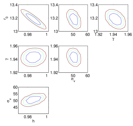
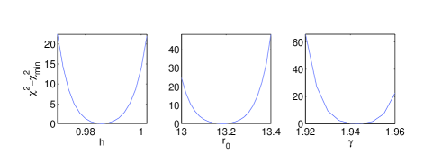
Figure 4 shows the resulting $\Delta\chi^{2}$ ($\Delta\chi^{2}=\chi^{2}-\chi^{2}_{min}$) in two-parameter space, with separate plots for each pair of parameters. In each of the panels, the curves represent the $\Delta\chi^{2}$ values after marginalization over the other two parameters. The one dimensional distributions, from $\Delta\chi^{2}$ values marginalized over the 3 other parameters (equation 17)are shown in Fig. 5. We find 1$\sigma$ statistical errors on $h,r_{0}$ and $\gamma$ of 0.5%, 0.4%, and 0.3% respectively. The important parameter for our purposes is $h$, for which we find a best fit value of $0.987$, which is $1.3\%$ ($\sim 2.5\sigma$) from the expected $h=1$. We attribute this percent level bias to the fact that the model correlation function we fit with is not a perfect match to the simulation correlation function. This type of systematic bias is likely to be difficult to circumvent. We return to this in the discussion (§5.2). The chi squared value for the best fit in this case is 578, for 494 bins, so while the fit is good, there is room for slight improvement.

We examine the $\xi(\sigma,\pi)$ plots from the simulation in Fig. 6, alongside the best fitting model $\xi$. In the top panel of Fig.  6 we have included only the measurement errors from hydrodynamic simulations, but assumed that the peculiar velocities have been subtracted. Although the velocity error distribtion is not Gaussian, we have fitted it in our convolution using a Gaussian function (equations 9 & 10), which has a best fitting $\sigma\sim 50km/s$ (see fig 4). By eye, it is difficult to see effect of these velocity errors making the $\xi(\sigma,\pi)$ anisotropic, although this effect sucessfully recovered in the fitting.

In order to judge the effect of peculiar velocities on a straight fit to the cosmic geometry, we have also tried fitting our 4 parameters without subtracting the peculiar velocities. By doing this, we will get an idea of how the peculiar velocities can mimic the effect of geometric distortions. This was addressed in the context of linear theory by Ballinger et al. (1996), who found the relationship governing the effective value of $h$ is $h\sim 1+2\beta$. Here $\beta=\Omega_{m}^{0.6}/b$, with $b$ being the bias parameter. In the present case, $b$ (the ratio of the cluster $\xi$ to the matter $\xi$) is $\sim 2.5$, so that $\beta\sim 0.2-0.4$ over redshifts from $z=0-1$. Based on this, we expect $h$ to be $\sim 1.4-1.8$ when peculiar velocities are not removed.

This simulation test was carried out, and $\xi(\sigma,\pi)$ is shown in the bottom panels of Fig.  6, alongside the best fitting model which includes geometric distortions only. We can see that the peculiar velocities cause a very strong distortion, and that the form of the distortion is not obviously different to the eye when compared to the geometric one, a point which has been made by many authors including Ballinger et al. (1996) and Matsubara and Suto (1996). When we fit the $h(z)$ that results (Fig. 7) we find values $\sim 1.6-1.8$, as expected. The $\chi^{2}$ per bin is 3.2 (1616 for 494 bins), which is substantially worse than the fit to true geometric distortions. This difference in the fit could be useful if accurate estimates of the peculiar velocities are not removed.

For example, a systematic overestimate of the velocity will cause the distortion $h(z)$ to be underestimated. In the worst case scenario detailed by Diaferio et al. 2005, using a naive measurement based on clusters unresolved in X-rays would result in an overestimate of the peculiar velocity of $20-50\%$. Subtracting these cluster velocities to recover an estimate of the real space correlation function would yield $h(z)$ values $\sim 0.1-0.35$ too low. This is at the level which would make an Einstein De Sitter model look like a concordance $\Lambda$ model, and so this would not result in an acceptable test of cosmic geometry. Even with a spatially resolved measurement of the temperature, from Diaferio et al. 2005 we would expect a bias in $h(z)$ of $\sim 5-10\%$, which would affect a measurement of $\Omega_{\Lambda}$ at the $\sim 0.1-0.2$ level. We note that Seghal et al. (2005) find somewhat more optimistic conclusions from a simulation study of constraining cluster parameters from SZ observations, finding that velocity errors could be biased by as low as $15-40{\rm\;km\;s^{-1}}$ if X-ray weighted temperature measurements are used. This said, there are also some improvements which could be made to reduce the bias, such as using the integrated SZ flux together with scaling relations (Benson et al. 2004), and/or making use of the $z$ dependence of the distortion more efficiently. As we have seen above, it is also possible that the relatively poor goodness of fit when peculiar velocity distortions remain will help diagnose this without a theoretical model for the peculiar velocities being necessary.

With presently planned surveys such as ACT and SPT, these biases will be comparable to or smaller than the statistical errors, however they will represent an severe obstacle to any attempt to use the cluster real space AP test as a precise probe of cosmology.

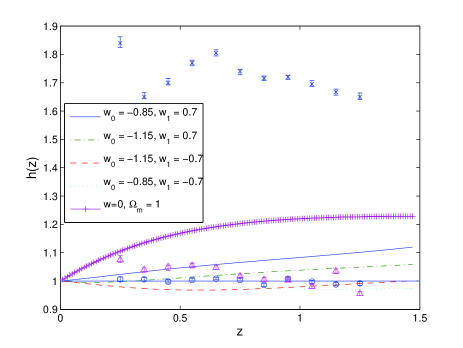
In Fig. 7 we also show $h$ vs. $z$ from our fitting to the simulation after subtracting peculiar velocities, but with the errors from hydrodynamic simulations. We can see that the expected result for LCDM, $h=1$ is recovered well, with error bars of $\sim 1\%$. The trend of $h(z)$ expected in some other example cosmologies is also shown as lines. The differences in $h(z)$ between an $\Omega_{m}=1$ model and LCDM are of the order of 10s of percent. Models with slightly different dark energy equations of state from LCDM fall even closer. We explore these below.

We have also carried out simulation tests using much larger peculiar velocity errors. For example, we have assigned random Gaussian distributed errors of $400{\rm\;km\;s^{-1}}$ to the clusters before carrying out our fitting procedure (Figure 3). In this case, we find values of $h(z)$ which are approximately $3\%$ too high, when averaged over the 10 redshift bins. This corresponds to a quite large bias, and means that it seems to be difficult to recover the correct cosmic geometry with such large velocity errors. With errors $\sim 200{\rm\;km\;s^{-1}}$, we find that the fitting technique works much better. Errors of this magnitude are to be expected given good observational data (see e.g., Diaferio et al. 2005, Seghal et al. 2005). We have not so far mentioned the errors on the cluster redshifts, but of course an additional complication is that they must also be measured to a comparably high level of precision.

Figure 7: Distortion parameter $h$ vs. $z$ for different cosmologies with repect to an $\Omega_{m}=0.3$, $\Omega_{\Lambda}=0.7$ cosmology. We show theoretical results for a few example cosmologies as lines ($\Omega_{m}=0.3$ unless noted otherwise). For the simulations, we show results as circles (with 1 $\sigma$ error bars) for the case with peculiar velocities corrected when random errors from hydrodynamic simulation are added. We also plot as triangles results for the simulations where much larger velocity errors were added (a Gaussian $\sigma$ of 400${\rm\;km\;s^{-1}}$) Finally, we also show results for the case where the peculiar velocities have been left in, as crosses, which yields an extremely distorted correlation function ($h$ very different from 1.)

3.2 Varying the dark energy equation of state

We adopt a simple equation of state, $w=w_{0}+w_{1}z$, where the pressure, $p=w\rho$. In order to find the best fit values for $w_{0}$ and $w_{1}$, we vary $w_{0}$, $w_{1}$ and $\Omega_{M}$ on a grid, and compute the expected $h(z)$ for each set of parameters. We then calculate $\Delta\chi^{2}$ by fitting to the simulation results in each redshift bin. $\chi^{2}$ is given by:

$$\chi^{2}=\sum^{n}_{i=1}\frac{(h_{i}-h^{\prime}_{i})^{2}}{\sigma^{2}}$$ (19)

where $h_{i}$ represents the best-fit distortion parameter $h$ in redshift bin $i$, $h^{\prime}_{i}$ is the distortion parameter with given $w_{0}$, $w_{1}$ and $\Omega_{M}$, and the sum is over $n$ bins in redshift. In Eqn 19, the $\sigma$’s have been obtained from the 1D marginalized results for $h(z)$ from the simulations (e.g. Figure 5). In the few cases where in the higher dimensional space before marginalization, the 1$\sigma$ contour for $h$ is out of the range, we are conservative and set the $\chi^{2}$ to a very large number so that during the marginalization the contribution to the likelihood from that point is negligible.

Figure 8: Fitting cosmological equation of state parameters (see §3.2) to the fiducial Hubble Volume simulation catalogue. Best fit at $w_{0}=-1.08,w_{1}=-0.15$. We show $1,2$ and $3\sigma$ contours. The top panel is without a prior on $\Omega_{m}$ and has a minimum at $\Omega_{m}=0.32$. The bottom is with a prior of $\Omega_{m}=0.3$, with uncertainty on $\Omega_{m}$ of $\sigma=0.05$. For visual purposes, a Gaussian filter with $\sigma=0.8$ grid cells was used to smooth before plotting.

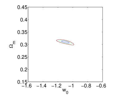
Once we have a 3d grid of $\Delta\chi^{2}$ values for $w_{0},w_{1}$ and $\Omega_{M}$ we marginalize over $\Omega_{m}$. We do this either with no external prior, or else after imposing a Gaussian prior on $\Omega_{m}$ ($\mathcal{L}^{\prime}=\mathcal{L}\exp^{-\frac{(\Omega_{m}-0.3)^{2}}{0.05}}$). We expect to recover $w_{0}=-1$, $w_{1}=0$, as this is the cosmology used in the Hubble volume simulation.

Figure 9: Distortion parameter $h(z)$ measured from the fiducial Hubble Volume simulations (points) together with the theoretical curve for the best fit $w_{0},w_{1}$ and $\Omega_{m}$ (which gives the minimum $\chi^{2}$ in Figure 8.) The line for the correct model $\Lambda$CDM is $h(z)=1$.

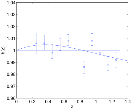
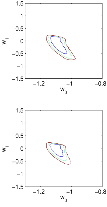
From our fitting procedure we find $w_{0}=-1.09^{0.022}_{0.022}$ and $w_{1}=-0.15^{0.29}_{0.17}$ with no prior imposed on $\Omega_{m}$ ($1\sigma$ error bars). Adding the prior makes little difference, with the best fit being $w_{0}=-1.09^{0.015}_{0.026}$ and $w_{1}=0.1^{0.05}_{0.27}$. In Figure 8 we show the $\Delta\chi^{2}$ contours for these two cases. Although we have seen from Figure 8 that the distortion parameter $h$ can be recovered at the percent level, this still translates into relatively loose constraints on $w_{1}$, regardless of the prior on $\Omega_{m}$.

In Figure 9 we show the shape of the theoretical $h(z)$ curve for this best fitting cosmology, compared to the measured values from the simulation. We can see that the best fit curve follows the dip in $h(z)$ values at high z, which account for the difference from the true cosmology.

Figure 10: Constraints on $w_{0}$ and $\Omega_{m}$ for the fiducial Hubble Volume simulation catalogue case when we set $w_{1}=0$. We show $1,2$ and $3\sigma$ contours. The cases with and without a prior on $\Omega_{m}$ give almost the same result. Best fit at $w_{0}=-1.09$ and $\Omega_{m}=0.31$.

In Figure 10 we set $w_{1}=0$, in order to assess the type of constraints possible in this case. We find a minimum $\chi^{2}$ at $\Omega_{m}=0.31^{0.002}_{0.002}$, and $w_{0}=-1.09^{0.020}_{0.037}$. Imposing the previous prior on $\Omega_{m}$ makes no difference to this result.

3.3 Test on the $\tau CDM$ simulation

We now test our method on a different simulated universe. In the previous case, have taken data sets from $\Lambda$CDM simulations, and then assumed the $\Lambda$CDM geometry when analyzing them. Because of this, we expected to recover a distortion parameter $h(z)$=1. Now instead, we use a different simulation, but still assume the $\Lambda$CDM geometry to analyze it. In this case, we expect to find $h(z)\neq 1$.

For the simulated universe, we use the Hubble volume simulation of the $\tau$CDM model (see Frenk et al 2000). This is a cosmology with $\Omega_{m}=1,\Omega_{\Lambda}=0$. The linear matter power spectrum has a similar shape to that of LCDM. We use all the clusters in an octant as before, except this time the maximum cluster redshift is $z_{max}=1.25$.

Figure 11: Theoretical distortion parameter $h(z)$ for $\tau$CDM and $\Lambda$CDM (lines). Data points with circles (crosses) represent fitted distortion parameters from the simulation with 1 $\sigma$ error bars for $\tau$CDM ($\Lambda$CDM).

We first compute the angular positions and redshifts of the clusters, as they would be seen by an observer. We then use the $\Lambda$CDM relations (Equations 5 and 6) to convert these into comoving coordinates, assuming an observer at the origin. We compute the correlation function from the simulation as before, and fit the distortion parameter $h(z)$.

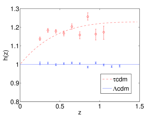
This test is is analogous to the real situation, where we would have observational data from an unknown cosmology and use an assumed cosmology during the fitting procedure. The unknown cosmology here is an Einstein-de Sitter universe with $\Omega_{m}=1$, and we find the distortion parameter with respect to a cosmology with $\Omega_{m}=0.3,\Omega_{\Lambda}=0.7$.

Using Equation 8 we compute the distortion parameter which we expect to recover in this case. This is shown as a dotted line in Figure 11. When we carry out the test, we find results which are intermediate between this line and the $h(z)=1$ LCDM line at all redshifts. This is an indication that in a realistic situation such as our test, the distortion parameter cannot be inferred simply when the assumed model (here LCDM) is very different from the actual Universe (in this case $\tau$CDM). Instead, if the distortion parameter is found to be very different from $h=1$, an iterative approach should be used. In this case, the assumed cosmology on the second try would be one intermediate between LCDM and $\tau$CDM. By using this method, we would approach the true cosmology, albeit more slowly. In Figure 11 we show the recovery of the Einstein-de Sitter geometry as points with error bars, using the EDS model as an assumed cosmology. This is representative of what should occur with the full iterative procedure, although this has not been fully tested in this case. We have rescaled the result for $h(z)$ by the ratio of the analytical predictions for $\Lambda$CDM and $\tau$CDM so that we can show the results on the same plot as the $\Lambda$CDM results. Although the fit is not quite as good as with the $\Lambda$CDM test, the results show that by moving towards an estimate of an assumed cosmology we can expect good results.

Figure 12: Distortion parameter $h(z)$ with 1 $\sigma$ error bars for the simulated SPT cluster survey. 3 example theory curves are shown as lines.

4 Results from simulated observational catalogues

4.1 The South Pole Telescope

The SPT survey will cover 4000 square degrees in 5 frequency bands and is expected to observe $\sim$20,000 clusters with masses greater than 2$\times 10^{14}{\rm M_{\odot}}$. For our SPT (and ACT, see below) simulations, we use a Gaussian measurement error of 100 $km/s$, based on published estimates of the best likely error on the kSZ velocity measurements (Nagai et al. 2004, Holder 2004, Sehgal et al. 2005). The standard deviation of errors from the hydrodynamic simulation which we used before in the Hubble volume case was $\sim 50km/s$, so the present value gives slightly bigger velocity distortions.

The simulation output we use to make our mock catalogue is an octant shape and covers almost the same area (we again use the $\Lambda CDM$ simulation), so to simulate the SPT survey we set a mass threshold so that the number of clusters that we observe is around 20,000. This means that the total number of clusters in the mock survey is only 1/40 of that in the underlying simulation. Since we have fewer clusters, we increase the size of each redshift bin and include clusters up to $z=1$ only. Our covariance matrix is constructed in the same way as in §3.1. When building the covariance matrix, we make sure that $\sigma,\pi$ bins are large enough that there are cluster pairs in each bin, to avoid singular error bars.

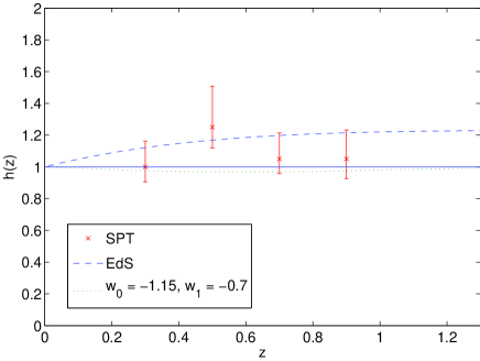
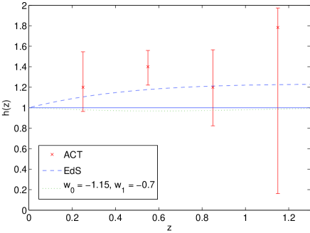
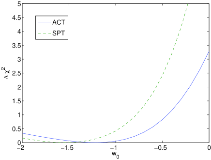
The results are shown in Figure  12. As expected, we have large error bars because of the of the smaller number of clusters than in the fully sampled simulation. The points also lie somewhat above the $h(z)=1$ curve, but the results still give a reasonable estimate of cosmic geometry without a large bias. Due to the large error bars, it is not possible to constrain $w_{0}$-$w_{1}$ within reasonable error bounds. However, by assuming that the dark energy density does not change with redshift, we can still find useful constraints on $\Omega_{\Lambda}$, and $w_{0}$, for example. In Figure 14 we show the constraints on $\Omega_{\Lambda}$ which result when a flat cosmology is assumed and $w_{1}=0$. We find 1 sigma errors on $\Omega_{\Lambda}$ of ${}^{+0.14}_{-0.09}$, and a central value within 1 $\sigma$ of the correct one. The constraints on $w_{0}$ (Figure 15) are weaker, with $w_{0}<-0.76$ at 1 $\sigma$.

Figure 13: Distortion parameter $h(z)$ with 1 $\sigma$ error bars for the simulated ACT cluster survey. 3 example theory curves are shown as lines.

4.2 The Atacama Cosmology Telescope

The ACT will cover only 200 square degree of the sky, but at higher sensitivity than the SPT. It is expected to observe $\sim 1000$ clusters with masses greater than $2\times 10^{14}{\rm M_{\odot}}$. With this mass threshold we find fewer cluster in the Hubble Volume simulation in a comparable area, so we use $10^{14}{\rm M_{\odot}}$ as our threshold. The $\chi^{2}$ analysis has been done in the same way as before with a Gaussian measurement error of 100 $kms$, except that the covariance matrix has been built using 6 separate volumes of 200 square degrees taken from the Hubble Volume octant. We then take one subvolume as our simulated survey and carry out our $\chi^{2}$ analysis using that.

Figure 14: Constraints on $\Omega_{\Lambda}$ for mock ACT and mock SPT surveys, assuming that $w_{1}=0$ and $\Omega_{m}+\Omega_{\Lambda}=1$.

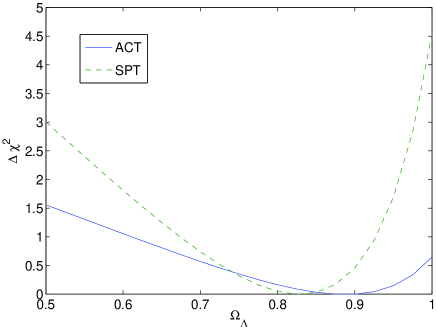
Since we now have even fewer clusters than in the mock SPT survey, the error bars are substantially larger (Figure  13). It is not possible to put any useful constraints in the $w_{0}$-$w_{1}$ plane without other priors. Again we we try to see if it is feasible to constrain $\Omega_{\Lambda}$ setting $w_{1}=0$ (Figure  14) and $w_{0}$ (Figure 15). We find 1 $\sigma$ errors on $\Omega_{\Lambda}$ $\sim 2$ times as large as for the mock SPT survey and a $1\sigma$ limit on $w_{0}<-0.45$.

From the analysis of ACT mock surveys we can see that the relatively small cluster sample and the need to split it up into redshift bins will make it difficult to measure the correlation function accurately enough to make this type of measurement. Nevertheless, some constraints will be possible, and the error bars of e.g. $\sim 0.2-0.3$ on $\Omega_{\Lambda}$ are still useful.

Figure 15: Constraints on $w_{0}$ for mock ACT and mock SPT surveys, assuming that $w_{1}=0$ and $\Omega_{m}+\Omega_{X}=1$.

5 Summary and Discussion

5.1 Summary

Using a combination of the Hubble Volume simulation (Frenk et al. 1999) and the hydrodynamic simulation results of Nagai et al. (2003), we have tested using the peculiar velocity corrected galaxy cluster correlation function to measure cosmic geometry. Our findings can be summarised as follows:
(1) The galaxy cluster correlation function, corrected using kSZ velocities can act as an intrinsically isotropic object for the AP test.
(2) The geometric distortion of the correlation function needs to be measured to $\%$ level accuracy in several redshift bins to constrain the equation of state parameter $w_{0}$ to better than $10\%$.
(3) Our simulation tests assuming errors from hydrodynamic modelling show that this can be done with a survey covering 1/8th of the sky, with clusters out to $z\sim 1$.
(4) The distortion from peculiar velocities will be very difficult to correct. Systematic over or underestimates of the peculiar velocities from kSZ measurements will be more problematic than statistical errors.
(5) Of surveys currently underway or planned, the SPT seems to be the most promising, and could yield constraints on $\Omega_{\Lambda}$ accurate to $10-20\%$.

5.2 Discussion

Of the many recent papers which have been written on using the AP test (e.g. Mc Donald et al. 2003), all take the approach of modelling the peculiar velocity component of the correlation function distortion. The fact that for galaxy clusters the peculiar velocity can be instead measured and subtracted offers the potential of a useful complementary method. For example, in order to model peculiar velocities well, the relationship between the clustering of the objects and the underlying mass field needs to be known to high precision. This is not necessary in the case where the velocities are subtracted. The latter method does however bring with it several new difficulties, including the necessarily sparse nature of galaxy cluster samples and the extremely challenging problem of measuring the peculiar velocities of thousands of clusters to high accuracy, when to date this has not yet been done for a single cluster.

One of the ingredients in our measurement of the distortion is our model for the correlation function as a function of separation $r$. We have found that using a fitting function which does not model the correlation function well can lead to biases in the measured distortion. For example, before adopting our fiducial fitting function, a power law combined with a CDM linear theory $\xi$, we tried a using single power law as the fitting function. This resulted in a systematic 10% bias in the value of $h(z)$. We also tried using a single power law to fit $\xi$ to regions $r=1\sim 40\;h^{-1}{\rm Mpc}$ (following da Ângela et al. 2005). In this case the fitted $h$ in each redshift bin changes slightly but the overall fitting of cosmological parameters does not improve very much. Using a more sophisticated fitting function than a power law therefore seems to be crucial.

The spectral distortion in the SZ effects is determined by $\tau$, $v_{pec}$ and $T_{e}$. These three parameters could be disentangled using multiwavelength observations. Sehgal et al. (2005) have shown how this will be possible in light of current survey sensitivities and suggest an independent temperature measurement from X-ray observations in order to break degeneracies. However, as mentioned in §2.5, the temperature obtained by X-ray spectroscopy for unresolved clusters is not the electron- weighted temperature which is required to separate three parameters ($\tau$, $v_{pec}$, $T_{e}$). Mathiesen & Evrard (2001) estimated that the discrepancy can be as much as 1keV. However, Sehgal et al. found that this temperature discrepancy will lead to a velocity bias of 15-40 km/s. They also claim that for an ACT-like survey, a 2 keV temperature error can still only lead to peculiar velocities with errors less than 100 km/s. We have found that the statistical measurement errors of this size can be modelled well, but that any systematic bias in the velocities will give biased results for cosmic geometry. This issue will need to be explored in more detail once large samples of clusters with kSZ measurements are available. Indeed, if the bias is too large, then it is possible that by assuming a model for cosmic geometry the distortion can be used instead to calibrate the peculiar velocities.

There many other planned surveys than ACT and SPT that are designed to be sensitive to SZ signals from clusters. For example, AMiBA, AMI ( $\sim 100$ clusters), APEX ($\sim 1000$ clusters) and Planck ($\sim 10000$ clusters). The Planck mission promises the largest survey area (the whole sky), compared to SPT for example which will observe 20,000 clusters over 4000 square degrees (about 1/8 of the sky). Planck will however have much larger CMB temperature measurement uncertainties, and so will only observe a similar number of clusters. They will therefore be distributed even more scarcely, making correlation function measurements difficult. We have tried sampling our simulation down to the space density of Planck clusters, but find that the Poisson errors on $\xi$ make it unfeasible to extract useful constraints on the geometric distortion.

In conclusion, we have shown that by subtracting kSZ measured velocities, it is possible to carry out a test of cosmic geometry with an intrinsically isotropic object, as envisaged in the original paper by Alock and Paczynski (1979). Using simulations we have seen that given small enough systematic and statistical errors, the correct geometry can be recovered. However, huge samples of galaxy clusters are required with precisely measured velocities. For example, to measure $w_{0}$ with 3% statistical errors we have seen that 800,000 clusters are necessary. As the kSZ signals are so small, observing the kSZ effects from this many clusters is not possible with currently planned surveys. However more advanced surveys are planned to detect more clusters in the future and the test we have proposed here will offer an additional way to use such data to constrain dark energy.

References

- (1) Aghanim N., Górski, K.M., Puget, J.-L. 2001, A&A, 374, 1., Lagache G., 2005, A&A, 439, 901
- (2) Aghanim N., Hansen S.H., Lagache G., 2005, A&A, 439, 901
- (3) Atrio-Barandela F., Kashlinsky A., Mücket J. P., 2004, ApJ, 601, L111
- (4) Alcock C., Paczyński B., 1979, Nat, 281, 358
- (5) Ballinger W.E., Peacock J.A., Heavens A.F., 1996, MNRAS282, 877
- (6) Bardeen, J., Bond,J.R., Kaiser, N. & Szalay,A.S. 1986, ApJ, 304, 15
- (7) Benson, B. A., Church, S. E., Ade, P. A. R., Bock, J. J., Ganga, K. M., Hinderks, J. R., Mauskopf, P. D., Philhour, B., Runyan, M. C. & Thompson, K. L. 2003, ApJ, 592, 674
- (8) Benson, B. A., Church, S. E., Ade, P. A. R., Bock, J. J., Ganga, K. M., Henson, C. N. & Thompson, K. L., 2004, ApJ, 617, 829
- (9) Birkinshaw, M., 1999, Phys. Rep., 310, 97
- (10) Blain, A.W., 1998, MNRAS, 297, 502
- (11) Borgani S. et al. , 1997, new Astron., 1, 321
- (12) Carlstrom J.E., Holder G.P., Reese E.D., 2002, ARA&A, 40, 643
- (13) Colberg J. M., White S. D. M., Yoshida N., MacFarland T. J., Jenkins A., Frenk C. S., Pearce F. R., Evrard A. E., Couchman H. M. P., Efstathiou G., Peacock J. A., Thomas P. A., 2000, MNRAS, 319, 209
- (14) Croft R.A.C., Dalton G.B., Esfstathiou G., 1999, MNRAS, 305, 547
- (15) da Ângela J., Outram P.J., Shanks T., Boyle B.Bj., Croom S.M., Loaring N.S., Miller L., and Smith R.Rj., MNRAS, 360, 1040
- (16) Croom S.M. et al. , 2005, MNRAS, 356, 415
- (17) Dalton G.B., Efstathiou G., Maddox S.J., Sutherland W.Wj., 1992, ApJ, 390, L1
- (18) Davis, M., and Peebles, P.J.E., 1983, ApJ, 267, 465
- (19) Diaferio A., Borgani S., Moscardini L., Murante G., Dolag K., Springel V., Tormen G., Tornatore L., Tozzi P., 2005, MNRAS, 356, 1477
- (20) Evrard A.E., MacFarland T., Couchman H.M.P., Colberg J.M., Yoshida N., White S.D.M. , Jenkins A., Frenk C.S., Pearce F.R., Efstathiou G., Peacock J.A., Thomas P.A., 2002, ApJ, 573, 7
- (21) Frenk C.S., Colberg J.M., Couchman H.M.P., Efstathiou G., Evrard A.E., Jenkins A., MacFarland T.J., Moore B., Peacock J.A., Pearce F.R., Thomas P.A., White S.D.M., Yoshida N., astro-ph/0007362
- (22) Forni, O., Aghanim, N., 2004, A&A, 420, 49
- (23) Hamilton A.J.S., 1992, ApJ, 385, L5
- (24) Hansen S.H., Pastro S., Semikoz D.V., ApJ, 573, L69
- (25) Hansen, S.H., 2004, astro-ph/0410004
- (26) Hawkins E. et al. , 2003, MNRAS, 346, 78
- (27) Hernández-Monteagudo C. Verde L., Jimenez R., Spergel D.N., 2006 ApJ653, 598
- (28) Hoyle F., Outram P.J., Shanks T., Boyle B.J., Croom S.M., Smith R.J., 2002, MNRAS332, 311
- (29) Hogg D., 1999, astro-ph/9905116
- (30) Haehnelt M.G., Tegmark M., 1996, MNRAS, 279, 545
- (31) Holder G.P., 2004, ApJ, 602, 18
- (32) Huchra J.P., Geller M.J., 1982, ApJ, 257, 423
- (33) Kaiser N, 1987, MNRAS, 1987, 227, 1
- (34) Kashlinsky, A., Atrio-Barandela, F. 2000, ApJ, 536, L67
- (35) Knox, L., Holder, G., and Church, S.E., 2004, ApJ,612, 96
- (36) Kravtsov A.V., Church S.E., Hoffman Y., 2002, ApJ, 571, 563
- (37) Lacey C., Cole S., 1994, MNRAS, 271, 676
- (38) Lange A. E., Church S. E., Holzapfel W., 1998, American Astronomical Society Meeting, 30, 908
- (39) Mathiesen B.F., Evrard A.E., 2001, ApJ, 546, 100
- (40) Matsubara T., Suto Y., 1996, ApJ, 470, L1
- (41) McDonald, P., 2003, ApJ, 585, 34
- (42) Mo H. J., White S. D. M., 1996, MNRAS, 282, 347
- (43) Mo H.J., Jing Y.P., White S.D.M., 1996, MNRAS, 282, 1096
- (44) Moscardini L, Matarrese S., Lucchin E., Rosati P., 2000, MNRAS, 316, 283
- (45) Nagai D., Kravtsov A., Kosowsky A., 2003, ApJ, 587, 524
- (46) Padilla N.D., Baugh C.M., 2002, MNRAS, 329, 431
- (47) Phillipps S., 1994, MNRAS, 269, 1077
- (48) Pointecouteau, E., Giard, M., Barret, D. 1998 A&A, 336, 44
- (49) Popowski P., Weinberg D., Ryden B., Osmer P., 1998, ApJ, 498, 11
- (50) Rephaeli Y., 1995ARA&A, 33, 541
- (51) Seo H.-J., Eisenstein D. J., 2003, ApJ, 598, 720
- (52) Sehgal N., Kosowsky A., Holder G., 2005, ApJ, 635, 22
- (53) Springel V. et al. , 2005, Nat, 435, 629
- (54) Sunyaev R.A., Zel’dovich Y. B., 1972, Comments Astrophysics and Space Physics, 4, 173
- (55) Sunyaev R.A., Zel’dovich Y. B., 1980, ARA& A, 18, 537
- (56) Vale, C. & White, M., 2006, New Astronomy, 11, 207
- (57) Zehavi I., et al. 2002, ApJ, 571, 172
- (58) Zehavi I., et al. 2005, ApJ, 630, 1