A longer XMM-Newton look at I Zwicky 1: Variability of the X-ray continuum, absorption, and iron K$\alpha$ line

Abstract

We present the second XMM-Newton observation ($85{\rm\thinspace ks}$) of the narrow-line Seyfert 1 galaxy (NLS1) I Zw 1 and describe its mean spectral and timing characteristics. On average, I Zw 1 is $\sim 35$ per cent dimmer in 2005 than in the shorter ($20{\rm\thinspace ks}$) 2002 observation. Between the two epochs the intrinsic absorption column density diminished, but there were also subtle changes in the continuum shape. Considering the blurred ionised reflection model, the long-term changes can be associated with a varying contribution of the power law component relative to the total spectrum. Examination of normalised light curves indicates that the high-energy variations are quite structured and that there are delays, but only in some parts of the light curve. Interestingly, a hard X-ray lag first appears during the most-distinct structure in the mean light curve, a flux dip $\sim 25{\rm\thinspace ks}$ into the observation. The previously discovered broad, ionised Fe K$\alpha$ line shows significant variations over the course of the 2005 observation. The amplitude of the variations is $25-45$ per cent and they are unlikely due to changes in the Fe K$\alpha$-producing region, but perhaps arise from orbital motion around the black hole or obscuration in the broad iron line-emitting region. The 2002 data are re-examined for variability of the Fe K$\alpha$ line at that epoch. There is evidence of energy and flux variations that are associated with a hard X-ray flare that occurred during that observation.

1 Introduction

I Zwicky 1 (I Zw 1; $z=0.0611$) is considered the prototypical narrow-line Seyfert 1 galaxy (NLS1) mainly due to its distinct optical properties. At X-ray energies the active galactic nucleus (AGN) exhibits behaviour that is somewhat more modest than for typical NLS1s (e.g. Leighly 1999a, 1999b). However, a short ($20{\rm\thinspace ks}$) XMM-Newton observation conducted in 2002 revealed a plethora of interesting characteristics, such as: hard X-ray flaring, unresolved transition array (UTA) absorption, and possibly multiple Fe K$\alpha$ emission lines (Gallo et al. 2004a, hereafter G04).

The discoveries in G04 prompted further examination with a second longer XMM-Newton observation. This is the first of three papers which describe the X-ray properties of I Zw 1 utilising all XMM-Newton data. In this work, we present an $85{\rm\thinspace ks}$ XMM-Newton observation and describe the mean spectral and timing characteristics of the AGN, as well as compare the data to the earlier 2002 observation. The complex ionised absorber and its long-term variability is discussed in detail in the work of Costantini et al. (2007). In addition, I Zw 1 exhibits remarkable short-term spectral variability during the 2005 observation. This is presented in Gallo et al. (2007).

2 Observations and data reduction

I Zw 1 was observed for the second time by XMM-Newton (Jansen et al. 2001) on 2005 July 18–19 during revolution 1027 (obsid 0300470101) (hereafter we will refer to this as the 2005 observation). The total duration was $85{\rm\thinspace ks}$, during which time all instruments were functioning normally. The EPIC pn (Strüder et al. 2001) and MOS (MOS1 and MOS2; Turner et al. 2001) cameras were operated in small-window mode with the medium filter in place. The Reflection Grating Spectrometers (RGS1 and RGS2; den Herder et al. 2001) also collected data during this time, as did the Optical Monitor (OM; Mason et al. 2001).

The Observation Data Files (ODFs) from the 2002 and 2005 observations were processed to produce calibrated event lists using the XMM-Newton Science Analysis System (SAS v7.0.0). Unwanted hot, dead, or flickering pixels were removed as were events due to electronic noise. Event energies were corrected for charge-transfer inefficiencies. EPIC response matrices were generated using the SAS tasks ARFGEN and RMFGEN. Light curves were extracted from these event lists to search for periods of high background flaring. Some background flaring is detected toward the end of the 2005 observation, and the data during those periods have been neglected. The total amount of good exposure time selected was $58{\rm\thinspace ks}$ and $82{\rm\thinspace ks}$ for the pn and MOS detectors, respectively. Source photons were extracted from a circular region 35^′′ across and centred on the source. The background photons were extracted from a larger off-source region and appropriately scaled to the source-selection region. Single and double events were selected for the pn detector, and single-quadruple events were selected for the MOS. The data quality flag was set to zero (i.e. events next to a CCD edge or bad pixel were omitted). The total number of source counts collected by the pn instrument in the $0.3-10{\rm\thinspace keV}$ range was approximately $2.75\times 10^{5}$. In the $0.5-10{\rm\thinspace keV}$ band, the MOS instruments collected about $8.4\times 10^{4}$ (MOS1) and $8.9\times 10^{4}$ (MOS2) source counts. Comparing the source and background spectra we found that the spectra are source dominated between $0.2-12{\rm\thinspace keV}$. The EPIC pn spectrum is analysed in the $0.3-10{\rm\thinspace keV}$ band where the calibration is most certain. To avoid cross-calibration uncertainties at low energies, the MOS spectra are neglected below $0.5{\rm\thinspace keV}$. The 2005 spectra from all instruments show relatively good agreement in these energy bands, within known calibration uncertainties (Kirsch 2006), so they are fitted simultaneously unless stated otherwise. As the broad-band light curve is less sensitive to calibration uncertainties, the data between $0.2-12{\rm\thinspace keV}$ are utilised.

The RGS were operated in standard Spectro+Q mode in 2005, and a total exposure of $85{\rm\thinspace ks}$ was collected. The RGS data are used in the analysis of the ionised absorber in I Zw 1 (Costantini et al. 2007) and will not be discussed here.

During 2005, I Zw 1 was observed with the OM in Fast-mode through four filters ($U$, $UVW1$, $UVW2$ and $UVM2$). The purpose was to examine possible optical variability. Unfortunately, the AGN was not well centred in the small, fast-mode frame and fell close to the detector edge. Consequently, optical variability could not be examined in a robust manner.

3 2005 X-ray light curves

During the $20{\rm\thinspace ks}$ 2002 observation I Zw 1 exhibited a modest X-ray flare, which lasted a total of $\sim 5{\rm\thinspace ks}$ (G04). Notably the flare appeared to be quite hard, concentrated in the $3-12{\rm\thinspace keV}$ band, thus inducing spectral variability. Aside from this lone event the light curve was relatively quiet in comparison to many NLS1.

The 2005 light curve appears more active, consistently variable with, on average, larger amplitudes than observed in 2002 (Figure 1). Perhaps the most interesting event in the light curve is the sharp drop about $25{\rm\thinspace ks}$ into the observation.

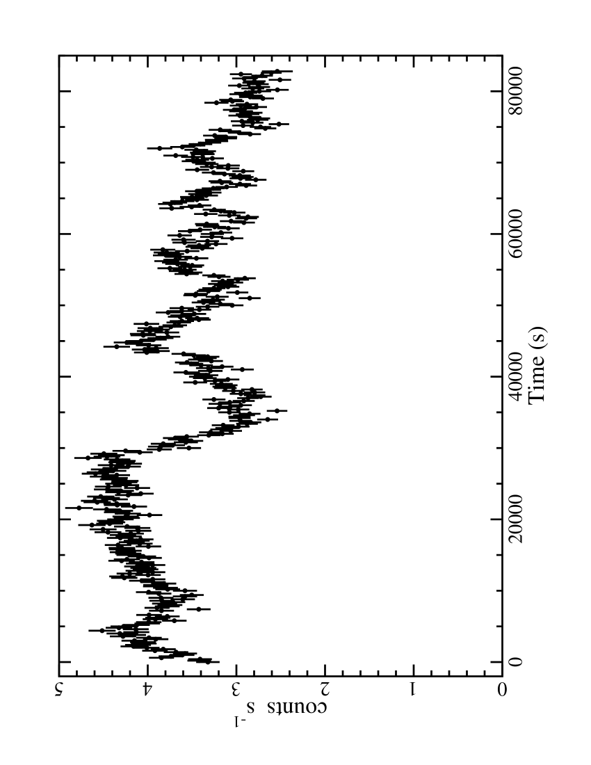
Figure 1: The 2005 $0.2-12{\rm\thinspace keV}$ EPIC pn light curve in $200{\rm\thinspace s}$ bins. The start time corresponds to the beginning of the pn exposure.

There is spectral variability related to the light curve, and this is discussed at length in Gallo et al. (2007). Here, we will focus on the flux variations.

Light curves were created in three EPIC pn energy bands: $0.2-0.7{\rm\thinspace keV}$, $2-3{\rm\thinspace keV}$ and $3-12{\rm\thinspace keV}$. Using the light curves in $1000{\rm\thinspace s}$ bins, each of the high-energy light curves was cross-correlated (following Edelson & Krolik 1988) with the the $0.2-0.7{\rm\thinspace keV}$ band to search for possible lags (positive delay means hard-band lags the soft-band). All of the cross-correlation functions (CCFs) were asymmetric toward positive lags (Figure 2). As will be demonstrated in the spectral analysis, the softest band is the region where both the power law component and the soft excess component influence the spectrum. Both higher bands are dominated by the power law component alone.

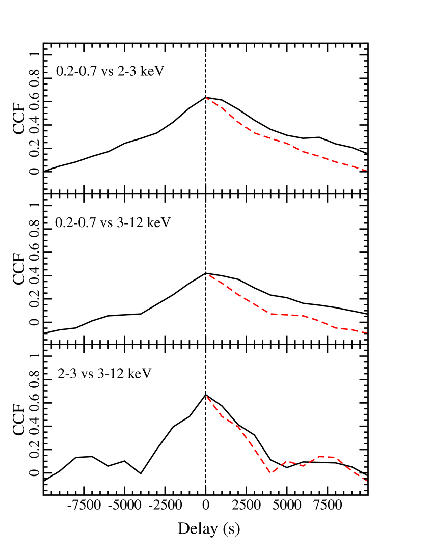
Figure 2: The CCF from cross-correlating the energy bands shown in each panel. In each panel the negative delay curve is reflected about the zero axis and shown as a red, dashed curve on the positive side. This is done to highlight the asymmetry of the CCFs toward positive lags meaning that the soft bands are leading the variations.

There are a few AGN where time delays as a function of Fourier frequency (see Nowak et al. 1999 and references therein for details) have been determined (see Papadakis et al. 2001 for the first reported detection in an AGN). If there were a single delay between the light curves in the various energy bands, then the time delay between all of the Fourier frequencies would be the same. In contrast, what is typically observed is that as the frequency of the Fourier components decreases, the delays increase. Furthermore, as the energy band separation between two light curves increases, the delays, at the same frequency, also increase (e.g. see Arévalo et al. 2006 for a recent discussion).

In the case of I Zw 1, we cannot estimate time lags as a function of frequency due to limited signal in the hard-band light curve. However, the CCFs are consistent with what we observe in other AGN and NLS1. The CCFs show broad humps around zero time lag with an asymmetry toward positive lags, but not a single, distinct delay. This is consistent with the hypothesis that in I Zw 1, just like in other Seyferts, the sine and cosine functions in the hard-band light curves are delayed with respect to those in the soft-band light curves, but the delay is not the same for all of them: the delays increase with decreasing frequency and increased separation between the energy bands.

Of interest may be the particularly small values measured in the CCFs ($0.5-0.7$). We examine this further by directly comparing light curves in each energy band normalised to their respective mean (Figure 3).

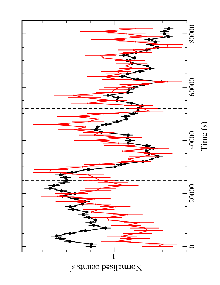
Figure 3: Light curves in the $0.2-0.7{\rm\thinspace keV}$ (black dots) and $3-12{\rm\thinspace keV}$ bands normalised to their respective means. A hard band lag is apparent in between $\sim 25-52{\rm\thinspace ks}$ (marked by the vertical dashed lines). The start time corresponds to the beginning of the pn exposure.

Most obvious in the comparison between the $0.2-0.7{\rm\thinspace keV}$ and $3-12{\rm\thinspace keV}$ band is the significance of the delay between $\sim 25-52{\rm\thinspace ks}$ (vertical dashed lines in Fig. 3). In particular, the delay seemingly begins at the onset of the sharp dip in the light curve. If we calculate the CCF in this time regime alone we see a clear dominant lag at $\sim 1{\rm\thinspace ks}$ (Figure 4).

However, as Figure 3 demonstrates, the lag is not always present. Sometimes there are no delays, and at other times the light curves show different behaviour and even anti-correlations (e.g. $\sim 20-25{\rm\thinspace ks}$ and $>75{\rm\thinspace ks}$ into the observation). All of these factors contribute to the small value of the CCF peaks. Similar behaviour was seen in the NLS1 IRAS 13224–3809 (Gallo et al. 2004b) where the authors suggested possible alternating lags between high- and low-energy bands (i.e. sometimes hard band lags and other times it leads).

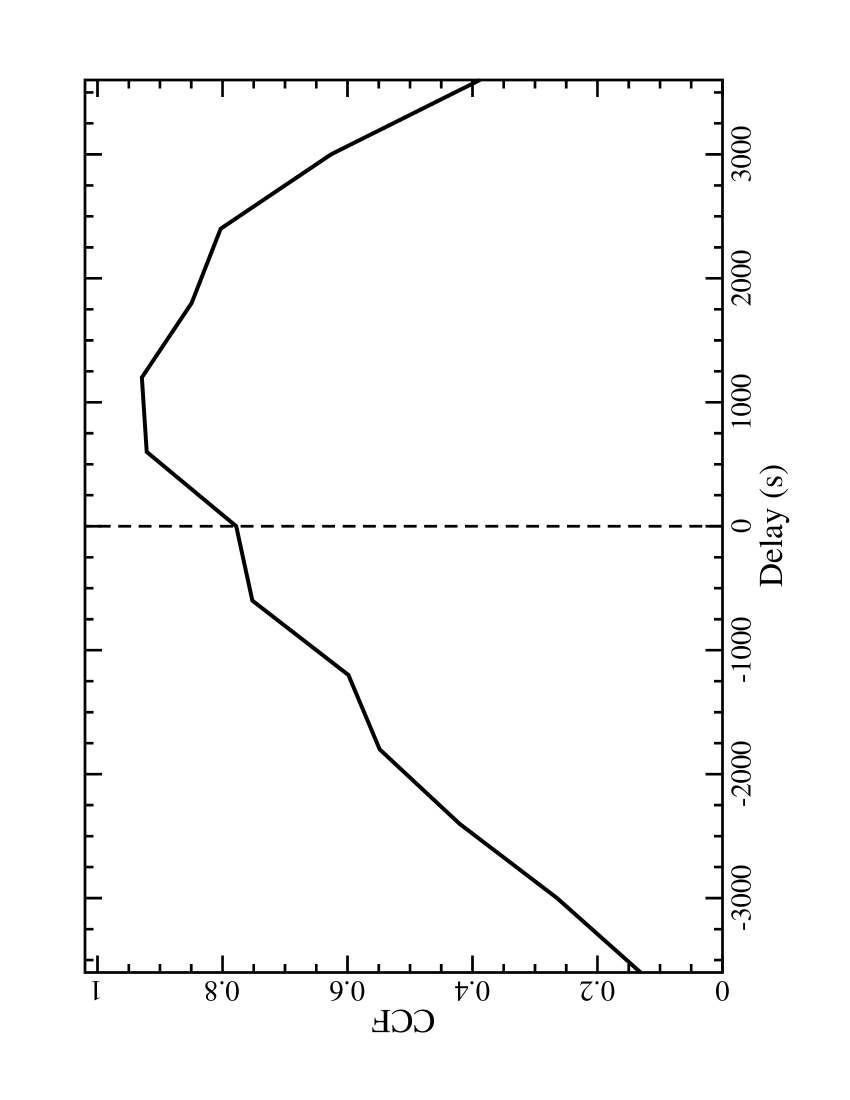
Figure 4: The CCF when cross-correlating the $0.2-0.7{\rm\thinspace keV}$ and $3-12{\rm\thinspace keV}$ light curves between $25-55{\rm\thinspace ks}$ only. A hard band lag appears more dominant in this time band and peaks at $\sim 1{\rm\thinspace ks}$.

4 2005 spectral modelling

The source spectra were grouped such that each bin contained at least 20 counts (typically more). Spectral fitting was performed using XSPEC v11.3.0 (Arnaud 1996). All parameters are reported in the rest frame of the source unless specified otherwise. The quoted errors on the model parameters correspond to a 90% confidence level for one interesting parameter (i.e. a $\Delta\chi^{2}$ = 2.7 criterion). A value for the Galactic column density toward I Zw 1 of $5.07\times 10^{20}\hbox{${\rm\thinspace cm}^{-2}\,$}$ (Elvis et al. 1989) is adopted in all of the spectral fits. K-corrected luminosities are calculated using a Hubble constant of $H_{0}$=$\rm 70\ km\ s^{-1}\ Mpc^{-1}$ and a standard flat cosmology with $\Omega_{M}$ = 0.3 and $\Omega_{\Lambda}$ = 0.7.

In the analysis of the 2002 data, G04 were able to fit the spectra with various phenomenological models, but could not distinguish a superior one. While they were able to establish that a second, soft component was a necessary part of the continuum they were unable to determine whether the soft excess was curved (e.g. blackbody-like) or flat (power law-like).

4.1 The 2-10 keVspectra

As was done for the 2002 data (G04), we built-up a broad-band spectral model for the 2005 observation utilising all the EPIC data. Fitting the $2-10{\rm\thinspace keV}$ EPIC spectra with a single power law (each instrument having free photon index ($\Gamma$) and normalisation to accommodate existing cross-calibration uncertainties) resulted in a satisfactory model (${\chi^{2}_{\nu}/{\rm dof}}=1.03/1090$). Adding a Gaussian profile to this continuum, with a common energy ($E$) and width ($\sigma$) among all three instruments was a significant improvement (${\Delta\chi^{2}}=59.5$ for 5 free additional parameters). The best fit line parameters were $E=6.70\pm 0.14{\rm\thinspace keV}$, $\sigma=523^{+276}_{-157}{\rm\thinspace eV}$ and $EW_{pn}=265^{+105}_{-32}$, $EW_{M1}=220^{+130}_{-49}$, $EW_{M2}=239^{+191}_{-79}{\rm\thinspace eV}$. G04 introduced the possibility of multiple line features in the Fe K$\alpha$ region of the 2002 spectrum, including an intrinsically narrow $6.4{\rm\thinspace keV}$ line. No such line is present in the 2005 spectrum. A narrow, neutral line is completely insignificant in the pn spectrum and any such feature in the MOS has an $EW<27{\rm\thinspace eV}$.

A comparable improvement (${\Delta\chi^{2}}=38.0$ for 5 free additional parameters) can be achieved if a disc line profile (Fabian et al. 1989) rather than a Gaussian profile is used for the broad residuals. In this case the best-fit energy and inner disc radius are $E=6.55^{+0.20}_{-0.10}{\rm\thinspace keV}$ and $R_{in}=6-26$ gravitational radii, respectively. The disc inclination ($i$) is fixed at $50^{\circ}$, to remain consistent with our finding in Section 6.1. Leaving the parameter free to vary does not enhance the fit statistics, nor does it affect the best-fit line energy. The line strength is $EW\approx 200{\rm\thinspace eV}$ in each spectrum. For simplicity, we adopt the Gaussian profile.

4.2 Simple broad-band models

Extrapolating the $2-10{\rm\thinspace keV}$ fit to $0.3{\rm\thinspace keV}$ in the pn and $0.5{\rm\thinspace keV}$ in the two MOS left a gradual rise in the residuals that is typically associated with the soft excess.

Table 1: Fit parameters for the simple models (column 1) applied to the 2005 full-band data. Fit quality is given in column 2. Neutral absorption intrinsic to I Zw 1 is given in column 3 ($\times 10^{20}\hbox{${\rm\thinspace cm}^{-2}\,$}$). In column 4, the continuum parameters are shown. If the parameter is not linked between the various instruments it is identified as pn, M1 (MOS1) and M2 (MOS2). $E_{b}$ is the break energy (in  keV) for the broken power law model. The photon index above ($\Gamma_{h}$) and below ($\Gamma_{s}$) the break energy are also shown. The blackbody temperature ($kT$) is given in  eV. Column 5 provides the absorption-edge parameters: energy ($E$) and optical depth ($\tau$). All fits except for the partial covering model (second row) include an FeK$\alpha$ emission line with comparable parameters to the results presented in the text. The line was not statistically necessary in the partial covering model. The parameters of the partial covering absorber, column density (${N_{\rm H}}_{pc}$, $\times 10^{22}\hbox{${\rm\thinspace cm}^{-2}\,$}$) and covering fraction ($f$), are given in column 6.

(1)	(2)	(3)	(4)	(5)	(6)
Model	${\chi^{2}_{\nu}/{\rm dof}}$	${N_{\rm H}}_{i}$	Continuum	Edge	Partial absorber
Single	$1.13/1628$	$0.71^{+0.23}_{-0.20}$	$\Gamma_{pn}=2.37\pm 0.01$	$E=644^{+9}_{-10}$
power law			$\Gamma_{M1}=2.29^{+0.02}_{-0.01}$	$\tau=0.15\pm 0.02$
			$\Gamma_{M2}=2.30^{+0.02}_{-0.01}$
Single	$1.08/1629$	$1.62^{+0.28}_{-0.31}$	$\Gamma_{pn}=2.43\pm 0.06$	$E=648^{+6}_{-9}$	${N_{\rm H}}_{pc}=31.5^{+7.6}_{-4.1}$
power law			$\Gamma_{M1}=2.35\pm 0.01$	$\tau=0.19\pm 0.02$	$f=0.72^{+0.09}_{-0.06}$
with partial covering			$\Gamma_{M2}=2.37\pm 0.01$
Broken	$1.08/1626$	$2.13^{+0.31}_{-0.38}$	$\Gamma_{s}=2.48\pm 0.03$	$E=648^{+6}_{-9}$
power law			$E_{b}=1.89^{+0.23}_{-0.10}$	$\tau=0.20\pm 0.02$
			$\Gamma_{h,pn}=2.27^{+0.02}_{-0.03}$
			$\Gamma_{h,M1}=2.17^{+0.03}_{-0.05}$
			$\Gamma_{h,M2}=2.35\pm 0.03$
Blackbody	$1.08/1626$	$<0.20$	$kT=216\pm 12$	$E=651^{+7}_{-9}$
plus			$\Gamma_{pn}=2.30\pm 0.01$	$\tau=0.20\pm 0.02$
power law			$\Gamma_{M1}=2.21\pm 0.01$
			$\Gamma_{M2}=2.23\pm 0.01$
Double	$1.04/1626$	$3.22^{+0.69}_{-0.27}$	$\Gamma_{1}=2.67^{+0.05}_{-0.04}$	$E=652^{+6}_{-10}$
power law			$\Gamma_{2,pn}=1.43^{+0.16}_{-0.06}$	$\tau=0.18\pm 0.02$
			$\Gamma_{2,M1}=1.74^{+0.12}_{-0.04}$
			$\Gamma_{2,M2}=2.03^{+0.13}_{-0.06}$

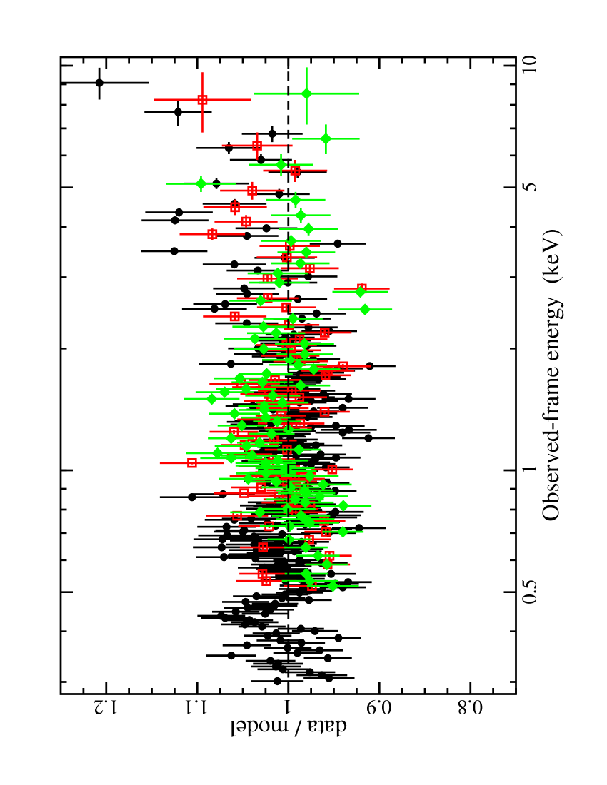
Figure 5: The residuals (data/model) from fitting a model composed of a blackbody, power law and Gaussian profile (modified by absorption) to the EPIC data (see third row in Table LABEL:tab:fits). Black dots, red open squares, and green diamonds correspond to the pn, MOS1, and MOS2 data, respectively. The data are rebinned for display purposes.

The entire 2005 $0.3-10{\rm\thinspace keV}$ band was modelled with various continuum models. Through repeated effort we found it necessary to include in all models an additional neutral absorber at the redshift of the source, as well as a low-energy ($\sim 650{\rm\thinspace eV}$) absorption edge that mimics the more complicated ionised absorption.

As with the 2002 observation, the 2005 data show that a second continuum component is required to fit the spectrum of I Zw 1 (see Table LABEL:tab:fits). According to an $F$-test, the addition of a second continuum component (i.e. 2 additional parameters) to a single power law is highly significant ($F$-test probability $\sim 10^{-17}$). Also like the 2002 observation, a single superior model does not stand out. However, there are similarities among all the models in Table LABEL:tab:fits. One may notice that the second component is not highly curved. Even in the case of the blackbody plus power law model, the high-temperature of the blackbody component will give it a flatter appearance in the EPIC bandpass.

Of interest is that there is detectable diminishing of the intrinsic column density in I Zw 1 since 2002. The exact change depends on what continuum model is assumed, but appears to be at least on the $50$ per cent level.

The residuals from the blackbody plus power law fit are shown in Figure 5. Notable in Figure 5 are the positive residuals, which remain in the fit above $\sim 8{\rm\thinspace keV}$. These residuals are apparent in all broad-band fits to the 2005 data (see also Figure 7 and the lower panel of Figure 8) , with the exception of the double power law model. The most likely cause is the significant spectral variability exhibited by I Zw 1 in 2005 (Gallo et al. 2007). Gallo et al. suggest that the power law photon index could be changing during the 2005 observation, which would explain the difficulty in fitting the average spectrum with a single power law. The reason that the residuals are minimal in the double power law model could simply be that the second power law does not begin to dominate the spectrum until rather high energies ($\sim 5.5{\rm\thinspace keV}$ in the pn spectrum).

Based on the blackbody plus power law model, the average $0.3-10{\rm\thinspace keV}$ flux during 2005, corrected for Galactic absorption, is $\sim 1.4\times 10^{-11}\hbox{${\rm\thinspace erg}{\rm\thinspace cm}^{-2}{\rm\thinspace s}^{-1}\,$}$. The luminosities in the $0.3-10{\rm\thinspace keV}$ and $2-10{\rm\thinspace keV}$ bands are $1.28\times 10^{44}\hbox{${\rm\thinspace erg}{\rm\thinspace s}^{-1}\,$}$ and $0.43\times 10^{44}\hbox{${\rm\thinspace erg}{\rm\thinspace s}^{-1}\,$}$, respectively. I Zw 1 is $\sim 35$ per cent dimmer than it was in 2002. For comparison, the estimated $2-10{\rm\thinspace keV}$ luminosity during the ASCA observation was $0.53\times 10^{44}\hbox{${\rm\thinspace erg}{\rm\thinspace s}^{-1}\,$}$ (Leighly 1999b).

5 A comparison of the 2002 and 2005 spectra

5.1 Summary of the 2002 observation

The $0.2-10{\rm\thinspace keV}$ spectrum of I Zw 1 has long been known to differ from those of other NLS1. It possesses a rather weak soft excess and is modified by intrinsic neutral and ionised absorption. The 2002 observation of I Zw 1 (G04) was rather typical of what had been seen previously (e.g. Leighly 1999a, b).

There were several simple continuum models (e.g. blackbody plus power law, broken power laws, multiple blackbodies plus power law) that when modified by intrinsic ionised absorption (an absorption-edge), neutral absorption (absorption column density) and an Fe K$\alpha$ emission line, fit the EPIC spectra adequately in 2002. None of these continuum models stood out as superior. Since the 2002 data were reprocessed with the newest calibration we refit the simple models to the newly processed data and find comparable results. The one modification was in the intrinsic absorption column density, which was slightly lower with the new calibration (${N_{\rm H}}=4.5\pm 0.5\times 10^{20}\hbox{${\rm\thinspace cm}^{-2}\,$}$ as opposed to ${N_{\rm H}}=10.0\pm 0.1\times 10^{20}\hbox{${\rm\thinspace cm}^{-2}\,$}$).

A particularly interesting spectral result from the 2002 observation was the possible presence of multiple iron lines. In addition to a broad and ionised line, the spectrum also required a narrow, unresolved emission line at $6.4{\rm\thinspace keV}$ . The most obvious interpretation adopted by G04 was that this feature was produced in distant material such as the torus, but an alternative interpretation is offered in Sect 8.4.2.

5.2 Spectral changes since 2002

The 2005 spectrum does appear substantially different from the 2002 observation. The broad-band differences between 2002 and 2005 can be depicted by extrapolating the best-fit $2-10{\rm\thinspace keV}$ power law to both spectra down to lower energies (Figure 6).

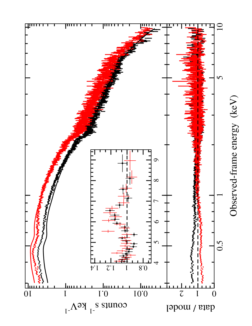
Figure 6: Top panel: Best-fit power law modelled to the 2002 (red marks, $\Gamma=2.28\pm 0.03$) and 2005 (black marks, $\Gamma=2.15\pm 0.02$) $2-10{\rm\thinspace keV}$ pn spectrum, and extrapolated to $0.3{\rm\thinspace keV}$. Lower panel: Resulting ratio from the above model. Top panel (inset): Ratio in the $4-9.5{\rm\thinspace keV}$ band, binned for display purposes.

The 2005 observation shows a much softer spectrum, a suggestion that the level of absorption may have changed since 2002. The best-fitting power law in the $2-10{\rm\thinspace keV}$ band is slightly flatter in 2005 ($\Gamma=2.15\pm 0.02$ compared to $\Gamma=2.28\pm 0.03$ in 2002), which likely also contributes to the apparently stronger soft excess at that epoch. The inset in Figure 6 shows the residuals in the Fe K$\alpha$ band. As with previous observations, the iron line appears broad and ionised. The agreement in the appearance of the iron line at both epochs is good.

We applied the blackbody plus power law model from 2002 to the 2005 data to examine consistency between the two epochs. Simply rescaling the model was unacceptable (${\chi^{2}_{\nu}/{\rm dof}}=5.7/846$). Allowing the level of neutral absorption to vary freely significantly improves the fit quality (${\chi^{2}_{\nu}/{\rm dof}}=1.27/845$) indicating that the column density of the neutral absorber has dropped in 2005 to ${N_{\rm H}}\approx 1.4\times 10^{20}\hbox{${\rm\thinspace cm}^{-2}\,$}$. Allowing the low-energy absorption edge to vary in energy and depth is a further improvement (${\Delta\chi^{2}}=36.2$ for 2 additional free parameters). The overall fit is not acceptable (${\chi^{2}_{\nu}/{\rm dof}}=1.23/843$) and demonstrates that subtle changes in the intrinsic continuum shape since 2002 may be appropriate.

If rather we consider a constant absorber and allow only the continuum parameters to vary, we obtain a worse fit (${\chi^{2}_{\nu}/{\rm dof}}=1.35/843$). Indeed variable absorbers seem necessary and are supported by the RGS data (Costantini et al. 2007).

6 A reflection interpretation for I Zw 1

6.1 The 2005 observation

The spectrum of I Zw 1 is power law dominated, but there is the necessity for a small contribution from a soft component below $\sim 2{\rm\thinspace keV}$. The ionised disc reflection model (Ross & Fabian 2005) blurred by relativistic effects has had relatively good success in duplicating the appearance of the soft excess (e.g. Crummy et al. 2006).

All the EPIC spectra were fitted with the blurred reflection plus power law model. As in the previous fits, we included an intrinsic neutral absorption component and an absorption edge as a pseudo-ionised absorber. Since the model is complex, to simplify the fitting process the normalisations of the MOS spectra were linked to the pn spectrum and only a constant scale factor was used to correct for possible flux offsets between instruments. The incident spectrum for the reflection component was linked to that of the power law component.

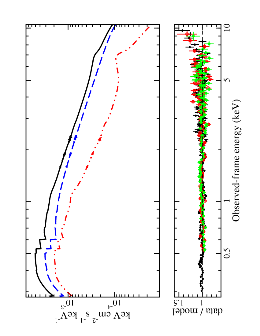
Figure 7: Top panel: The best fit blurred reflection model (only the pn model is shown for clarity). The reflection (red, dash-dot curve) and power law (blue, dashed curve) components, which make up the combined fit (black, solid curve) are presented. Bottom panel: The residuals of the model to the EPIC spectra. Symbols are as defined in Figure 5.

Table 2: The blurred reflection and power law model (with absorption) applied to the 2005 EPIC spectra (${\chi^{2}_{\nu}/{\rm dof}}=1.10/1627$). The absorption parameters are as defined in Table LABEL:tab:fits. The blurring parameters are the emissivity index ($\alpha$); inner ($R_{in}$) and outer ($R_{out}$) disc radius in gravitational radii (${\thinspace r_{\rm g}}=GM/c^{2}$); and disc inclination ($i$). The iron abundance and ionisation parameter ($\xi=4\pi Fn^{-1}$, where $F$ is the total incident flux and $n$ is the hydrogen number density) of the reflector are also given.

(1)	(2)
Model Component	Fit Parameter
Absorption	${N_{\rm H}}_{i}=1.05^{+0.07}_{-0.13}\times 10^{20}\hbox{${\rm\thinspace cm}^{-2}\,$}$
(neutral and	$E=638^{+7}_{-3}{\rm\thinspace eV}$
ionised)	$\tau=0.30\pm 0.01$
Power law	$\Gamma=2.24\pm 0.01$
Blurring	$\alpha=2.48^{+0.36}_{-0.31}$
	$R_{in}=5.0^{+8.2}_{-1.6}{\thinspace r_{\rm g}}$
	$R_{out}=200{\thinspace r_{\rm g}}$ (fixed)
	$i=51\pm 2^{\circ}$
Reflector	Fe$=1.1\pm 0.1$ solar
	$\xi=3060^{+107}_{-186}{\rm\thinspace erg}\hbox{${\rm\thinspace cm}{\rm\thinspace s}^{-1}\,$}$

The fit quality is not as satisfactory as some of the simple models (${\chi^{2}_{\nu}/{\rm dof}}=1.10/1627$), but it does have the advantage of offering a physical explanation for the origin of the soft excess and broad Fe K$\alpha$ line. Fit parameters are shown in Table LABEL:tab:reffit, and the model along with fit residuals are presented in Figure 7. The fraction of reflected-to-total flux in the $0.3-10{\rm\thinspace keV}$ range (corrected for Galactic and source absorption) is $\sim 0.30$. Drawing conclusions from the fit parameters should probably be done with caution given the complexity of the low-energy absorption. However, it can be noted that the disc inner radius is not extremely small ($R_{in}=5.0^{+8.2}_{-1.6}{\thinspace r_{\rm g}}$) and the emissivity profile is not very steep ($\alpha=2.48^{+0.36}_{-0.31}$). Both points suggest that the reflection component does not necessarily originate from the innermost confines around the black hole as is suggested for many NLS1.

The advantage of this model is that it can account for the iron emission and soft excess in a self-consistent manner. Moreover, as will be discussed in Gallo et al. (2007), this reflection scenario can potentially explain some of the complicated spectral variability exhibited by I Zw 1.

6.2 Simultaneous fit to the 2002 and 2005 data

Based on the investigation in Section 5.2, most of the spectral differences between 2002 and 2005 can be associated with changes in the level of absorption. However, there do appear to be subtle changes in the shape of the continuum as well. As I Zw 1 was nearly twice as bright in 2002, in terms of the blurred reflection model the changes in the continuum shape could be interpreted as differing contributions from the direct power law component.

The data from both epochs were fitted simultaneously to examine consistency in the reflection scenario. For simplicity, many parameters were fixed to the best-fit 2005 values (see Table LABEL:tab:pnref). The primary parameters that were left free for each dataset were the power law and absorption parameters, and the normalisation of the reflection component. The iron abundance and disc inclination were linked between the two spectra as large changes in these parameters would not be expected over 3-years. A reasonable fit can be achieved (${\chi^{2}_{\nu}/{\rm dof}}=1.06/1480$) in this manner (see Figure 8 and Table LABEL:tab:pnref).

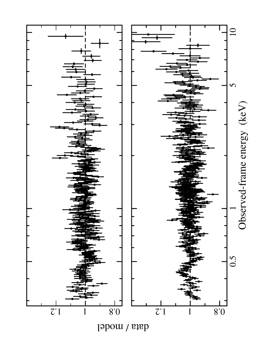
Figure 8: Residuals from a self-consistent power law plus blurred reflection model fitted simultaneously to the pn data from 2002 (top panel) and 2005 (bottom panel).

Table 3: The blurred reflection and power law model (with absorption) applied simultaneously to the 2002 and 2005 pn spectra (${\chi^{2}_{\nu}/{\rm dof}}=1.06/1480$). The parameters are as defined in Table LABEL:tab:reffit and $f$ marks the ones that are fixed in the fit. The 2002 and 2005 values are given in columns (2) and (3), respectively. The reflection ($R$) and flux fractions ($F_{R}$) (as defined in the text) are given in the final two rows.

(1)	(2)	(3)
Model Component	2002	2005
Absorption	${N_{\rm H}}_{i}=4.38^{+0.20}_{-0.19}$	$0.22^{+0.14}_{-0.17}\times 10^{20}\hbox{${\rm\thinspace cm}^{-2}\,$}$
(neutral and	$E=623\pm 10$	$634^{+11}_{-6}{\rm\thinspace eV}$
ionised)	$\tau=0.30^{+0.03}_{-0.04}$	$0.23\pm 0.02$
Power law	$\Gamma=2.28\pm 0.02$	$2.21^{+0.10}_{-0.08}$
Blurring	$\alpha=2.48^{f}$	$2.48^{f}$
	$R_{in}=5.0^{f}$	$5.0^{f}{\thinspace r_{\rm g}}$
	$R_{out}=200^{f}$	$200^{f}{\thinspace r_{\rm g}}$
	$i=58\pm 3$	$58\pm 3$
Reflector	Fe$=1.10\pm 0.13$	$1.10\pm 0.13$ solar
	$\xi=3060^{f}$	$3060^{f}{\rm\thinspace erg}\hbox{${\rm\thinspace cm}{\rm\thinspace s}^{-1}\,$}$
$R$	$0.27\pm 0.04$	$0.45\pm 0.04$
$F_{R}$	$0.22\pm 0.03$	$0.31\pm 0.03$

As is seen in Table LABEL:tab:pnref there is no strong indication for a change in the shape of the direct power law component between 2002 and 2005. In addition, most of the blurring and reflection parameters have been fixed. The most notable changes are in the amount of absorption (as noted in previous fits and by Costantini et al. 2007), the reflection fraction ($R$, fraction of reflected emission to power law emission in the $0.3-10{\rm\thinspace keV}$ band), and in the level at which the reflection component contributes to the total $0.3-10{\rm\thinspace keV}$ spectrum ($F_{R}=0.22\pm 0.03$ in 2002 and $0.31\pm 0.03$ in 2005).

7 Iron line variability

7.1 FeK$\alpha$ variability during the 2005 observation

In the analysis of G04 there were indications that the broad feature in the 2002 observation was composed of multiple (at least two) narrower emission lines. In the 2005 observation, the residuals can be fit by a single Gaussian profile. Based on the width of the line ($\sigma=523^{+276}_{-157}{\rm\thinspace eV}$) in the EPIC spectra, the line-emitting region is between $12-66{\thinspace r_{\rm g}}$. Similar distance estimates come from the disc line fit and the blurred reflection model. Given the long observation and proximity of the line emitting region makes it plausible to search for line variability.

The mean pn spectrum was divided into 17 segments, each of $5{\rm\thinspace ks}$. The exposure in each segment was $\sim 3.5{\rm\thinspace ks}$, taking account of the live-time of the pn camera in small window mode. The average number of source counts in the $5.0-7.2{\rm\thinspace keV}$ band was slightly more than $300$. The counts were grouped into spectra such that each bin contained at least 20 counts. For each $5{\rm\thinspace ks}$ spectrum the continuum was determined by fitting the $4-10{\rm\thinspace keV}$ band with a power law, while excluding the $5-7.2{\rm\thinspace keV}$ range. The omitted band was replaced and the spectrum was rebinned into channels of $250{\rm\thinspace eV}$. Excess counts above the continuum in each $250{\rm\thinspace eV}$ bin were recorded. From this information an excess residual image was created as illustrated in Iwasawa et al. (2004; and in prep). The result is analogous to modelling each spectrum with a power law plus Gaussian profile and measuring the flux in the Gaussian component. The advantage of creating an excess residual image is that we can circumvent the limitations of working in the Poisson regime, thus making trends in the variations of the line-flux more visible.

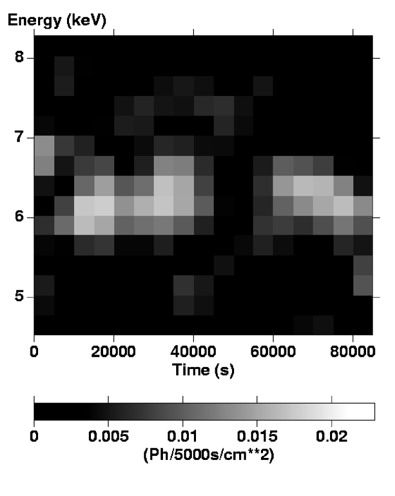
Figure 9: Excess-residual image for the 2005 pn spectrum in the $4.5-8.2{\rm\thinspace keV}$ band. Bright spots indicate positive residuals in the spectrum, above a power law continuum. The time resolution is $5{\rm\thinspace ks}$, and the spectra are binned into $250{\rm\thinspace eV}$ wide channels. The bright band between $5.8-6.7{\rm\thinspace keV}$ corresponds to the broad emission line seen in the mean spectrum. The feature appears to be variable over the course of the observation.

The resulting image from the 2005 observation is shown in Figure 9 and clearly indicates that the broad-line flux is variable. Most notably, the line flux diminishes significantly $45-60{\rm\thinspace ks}$ from the start of the observation.

To create a light curve from the image, the excess counts between $5.8-6.7{\rm\thinspace keV}$ were accumulated. Uncertainties on the light-curve data points were estimated from Monte Carlo simulations of the excess residual image.

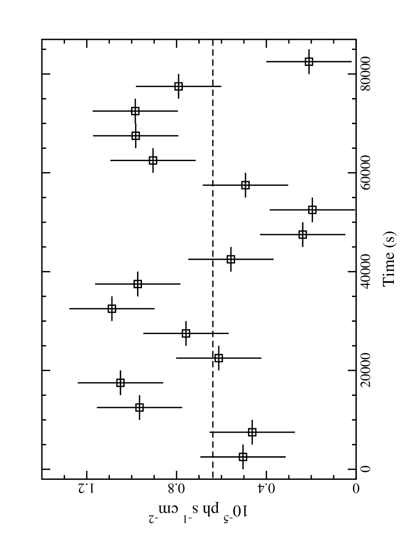
Figure 10: The light curve of the broad Fe K$\alpha$ emission in I Zw 1 during the 2005 observation. Bins are $5{\rm\thinspace ks}$. The 1-$\sigma$ uncertainties were estimated as described in the text. A constant fit is shown for comparison.

One-thousand images were created in an identical manner as done for I Zw 1. The spectra from which the images were derived were simulated for identical conditions as the 2005 observation, assuming a power law plus stationary Gaussian profile. The uncertainty in the observed light curve was taken to be the standard deviation in the excess counts resulting from the simulated images. Details of the process including caveats are discussed in Iwasawa et al. (2004).

The Fe K$\alpha$ light curve shows clear variability (Figure 10) with a constant fit being unacceptable ($\chi^{2}_{\nu}=2.45$). The fractional variability amplitude (${F_{\rm var}}$, using uncertainties derived in Edelson et al. 2002) is $34.8\pm 9.7$ per cent.

A light curve of the $6-10{\rm\thinspace keV}$ continuum was generated based on the power law fits used to derive the Fe K$\alpha$ light curve. The uncertainties in the $6-10{\rm\thinspace keV}$ flux were assumed to be the same as the uncertainty in the corresponding count rate. The continuum light curve, normalised to its average flux, is shown in Figure 11 with the broad-line flux light curve (Figure 10), normalised to its average flux, overplotted as a dashed curve.

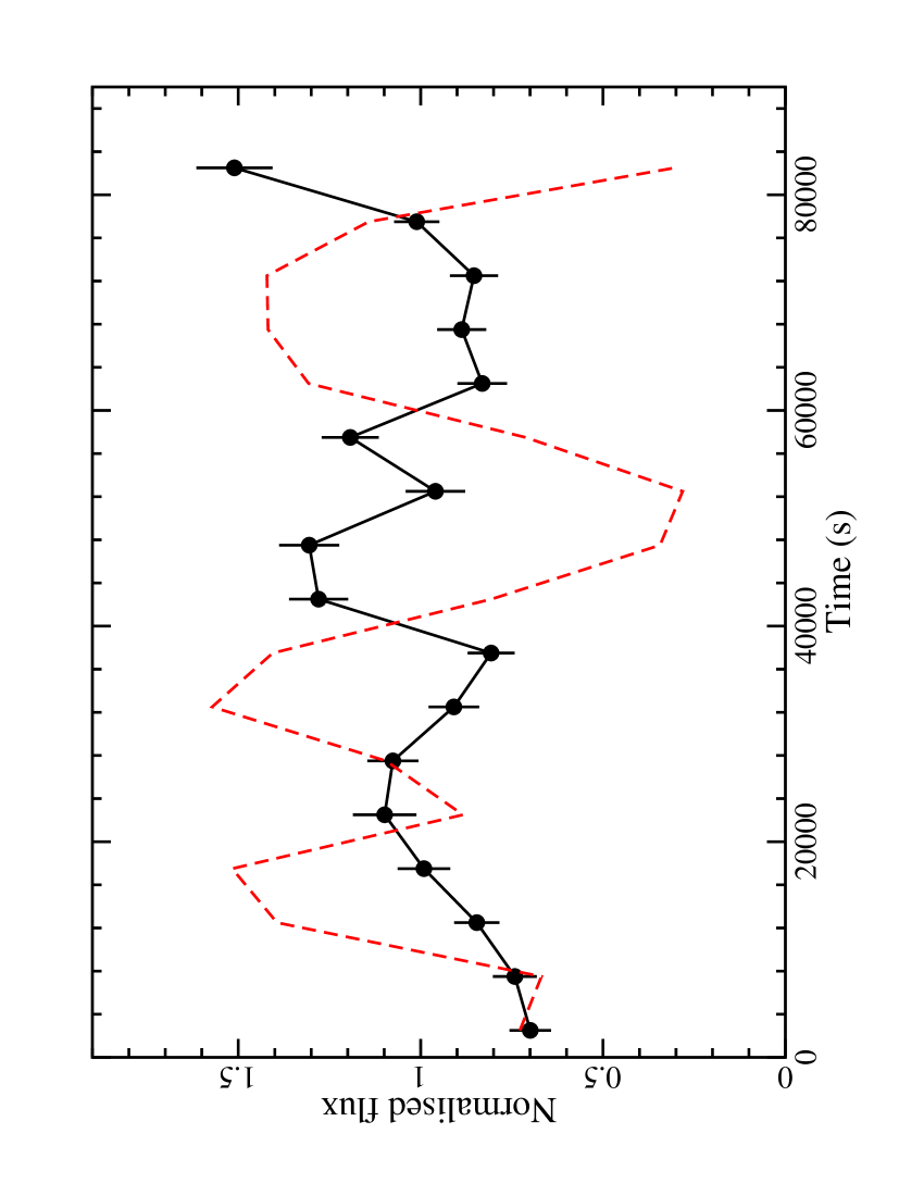
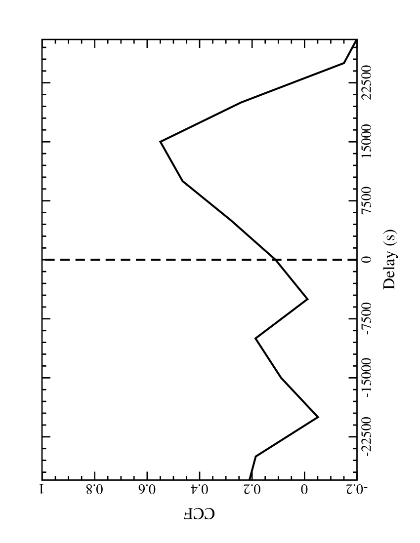
Figure 11: Top panel: The $6-10{\rm\thinspace keV}$ light curve of the continuum used to establish the iron line variations, normalised to its average flux. The FeK$\alpha$ data shown in Figure 10 are normalised to the average FeK$\alpha$ flux and overplotted (red, dashed curve). Bins are $5{\rm\thinspace ks}$. The 1-$\sigma$ uncertainties on the continuum data points are taken from the $6-10{\rm\thinspace keV}$ count rate. Lower panel: The CCF of the two light curves shown in the top panel. A positive delay indicates that the continuum changes lead the emission line variations.

Interestingly, the curves appear to be anti-correlated in some parts of the light curve. Cross-correlating the broad-line and $6-10{\rm\thinspace keV}$ continuum light curves indicates a weak correlation with the broad-line light curve lagging the continuum fluctuations by $\sim 15{\rm\thinspace ks}$ (lower panel Figure 11).

The fractional variability in the $6-10{\rm\thinspace keV}$ continuum is ${F_{\rm var}}=20.8\pm 4.0$ per cent, less than the ${F_{\rm var}}$ in the Fe K$\alpha$ line. Statistically, the amplitude of the continuum variations is consistent with the Fe K$\alpha$ variations within about 2-$\sigma$. However, the difference is likely larger since the uncertainties on ${F_{\rm var}}$ are conservatively over-estimated (Edelson et al. 2002).

7.2 Revisiting the Fe K$\alpha$ variability in 2002

In fitting the spectra in various segments of the 2002 observation, G04 found little evidence of intensity variations in the broad-line. We take advantage of the excess-residual technique to re-examine the broad-line variability in the 2002 observation. An excess-residual image has been created for the 2002 pn observation in a nearly identical manner as was done for the 2005 observation. The only difference is that the time resolution is slightly better during 2002 because the mean spectrum was divided into 6 segments of $3.6{\rm\thinspace ks}$ each (rather than $5{\rm\thinspace ks}$). This can be done without degrading the data quality because the I Zw 1 was brighter in 2002 and because the observation was conducted in large-window mode, which has a CCD live-time of $\sim 95$ per cent; therefore the actual exposure in each segment of the 2002 observation is almost the same as the exposure in each segment of the 2005 data.

Figure 12: Excess-residual image for the 2002 pn spectrum in the $4.5-8.2{\rm\thinspace keV}$ band. Bright spots indicate positive residuals in the spectrum, above a power law continuum. The time resolution is $3.6{\rm\thinspace ks}$, and the spectra are binned into $250{\rm\thinspace eV}$ wide channels. The bright band between $6.0-6.5{\rm\thinspace keV}$ corresponds to the broad emission line seen in the mean spectrum. Between $10-15{\rm\thinspace ks}$ there is also brightening in the $5.5-6.0{\rm\thinspace keV}$ band.

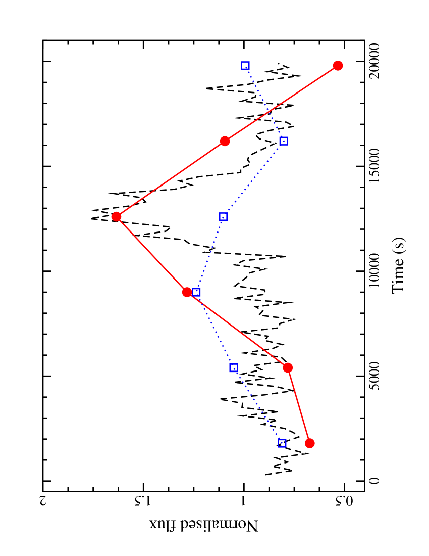
Figure 13: Various light curves from the 2002 observation of I Zw 1 normalised to their respective averages. The black, dashed curve is the $3-12{\rm\thinspace keV}$ continuum light curve highlighting the hard X-ray flare reported previously by G04 (uncertainties in the curve are found in G04). The filled, red circles connected by a solid line mark the light curve extracted from the residual image (Figure 12) in the $5.5-6.0{\rm\thinspace keV}$ range (i.e. the red line). The peak intensity in the red line corresponds with the peak intensity in the $3-12{\rm\thinspace keV}$ continuum light curve. The open, blue squares connected by a dotted line is the light curve extracted from the residual image in the $6.0-6.5{\rm\thinspace keV}$ band (i.e. the blue line).

The 2002 excess-residual image is shown in Figure 12. The broad-line is dominant in the $6.0-6.5{\rm\thinspace keV}$ range, but there is also apparent brightening that occurs in the $5.5-6.0{\rm\thinspace keV}$ band between $10-15{\rm\thinspace ks}$. This is of particular interest because the continuum light curve shows a hard X-ray flare that peaks during this time interval (see G04).

Light curves were extracted from the excess-residual image in the $6.0-6.5{\rm\thinspace keV}$ (blue line) and $5.5-6.0{\rm\thinspace keV}$ (red line) bands. They were then normalised to their respective means and plotted with the normalised 2002 $3-12{\rm\thinspace keV}$ continuum light curve (Figure 13). As the observation was so short uncertainties in the residual-image light curves were not derived in a robust manner as was done for the 2005 data. We also note that propagation of Poisson uncertainties in each data bin yields very large error bars (on the order of 100 per cent), therefore we are only illustrating a trend in Figure 13.

The light curves suggest that the variations are more intense in the $5.5-6.0{\rm\thinspace keV}$-line than in the $6.0-6.5{\rm\thinspace keV}$-line. There also is no obvious connection between the $6.0-6.5{\rm\thinspace keV}$-line light curve and that of the continuum. On the other hand, the $5.5-6.0{\rm\thinspace keV}$ variations appear to be well correlated with the high-energy continuum variations and, despite the unknown size of the true error bars in the $5.5-6.0{\rm\thinspace keV}$-line light curve, the trend is obvious.

8 Discussion

8.1 I Zw 1: a not so prototypical NLS1 in X-rays?

The strong Fe ii emission in the optical spectrum of I Zw 1 was noted a half century ago (Sargent 1968), and given the intensity and narrowness of the lines the AGN became a laboratory for Fe ii studies (e.g. Phillips 1976, 1977, 1978; Boroson & Green 1992; Laor et al. 1997; Vestergaard & Wilkes 2001). Its narrow Balmer lines were also noted fairly early on (e.g. Oke & Lauer 1979).

When a formal definition of the NLS1 class was established (Osterbrock & Pogge 1985), based on optical spectral properties, it was realised that I Zw 1 was already the best-studied member of this class of AGN, likely leading to its labelling as the prototype NLS1. However, some X-ray properties are also characteristic of NLS1s and I Zw 1 does not exhibit all these qualities to noticeable levels. In fact, in some instances I Zw 1 even displays behaviour that is atypical of the class. For example, I Zw 1 is observed through a column density intrinsic to the AGN. This is unusual for NLS1s (e.g. Boller, Brandt & Fink 1996), but also for type 1 AGN in general.

The soft excess emission above the underlying steep power law is weak in I Zw 1 compared to most NLS1s, and not because of the relatively high intrinsic absorption (e.g. Leighly 1999b, Tanaka et al. 2005). Even the clear detection of a broad Fe K$\alpha$ emission line in I Zw 1 seems unusual given that NLS1s appear not to show broad emission lines so obviously (e.g. Fabian et al. 2002, 2004; Guainazzi et al. 2006).

The identification of I Zw 1 as the prototype NLS1 originated due to its well-studied optical properties, but it now lingers mainly as a historic perspective. It can even be argued that some of its X-ray properties are atypical of the norm.

8.2 Time lags

The average CCFs calculated in Section 3 show a tendency for positive lags (hard band following soft band). This phenomenon has been observed in other AGN (e.g. Arévalo et al. 2006 and references therein) and Galactic black holes (e.g. McClintock & Remillard 2005). However the origin of the lags is not certain.

In a simple corona with a uniform temperature and optical depth, variations can result from fluctuations in the intensity of the seed photons. Variations of this nature should produce fixed delays between low- and high-energy bands, resulting in a common time delay for all Fourier components. We do not estimate time lags as a function of frequency in I Zw 1; however the broad, asymmetric CCFs suggest that we do not have a single, well defined delay between the various energy bands. Examination of normalised light curves in different energy bands further supports this. A time lag is only seen in parts of the light curves. In fact, at times the light curves are not correlated, or are actually anti-correlated.

Lags are seen in Cyg X-1, which can be attributed to spectral evolution in magnetic flares as they detach from the accretion disc (e.g. Poutanen & Fabian 1999). Another possibility is that the lags are manifested by material that propagates toward the black hole from regions of soft X-ray emission to regions of hard X-ray emission (e.g. Böttcher & Liang 1999; Kotov et al. 2001).

Based on the observation of another NLS1, IRAS 13224+3809, Gallo et al. (2004b) claimed a lag that alternated (sometimes hard band followed other times it led), with possible dependency on the average flux of the source. There is likely similar behaviour here as the first notable lag coincides with a sharp flux dip in the light curve about $25{\rm\thinspace ks}$ into the observation.

8.3 Diminished neutral absorption since 2002

Significant variations in the low-energy spectra of some Seyfert 1 galaxies have been previously observed and interpreted as changes in the low-energy continuum component (e.g. Page et al. 2002, Starling et al. 2004). In the case of I Zw 1, this does not appear to be the most straightforward explanation. There is detectable diminishing of the intrinsic column density in I Zw 1 since 2002. The exact change depends on what continuum model is assumed, but appears to be at least on the $50$ per cent level.

Changes in the neutral column density have been reported in several type 2 (i.e. absorbed) AGN (e.g. Risaliti et al. 2002), but to the best of our knowledge not in a NLS1. I Zw 1 is a merging and starburst system so there are several sources of absorption that exist in the galaxy and could feasibly change (e.g. due to bulk motion or dissipation of an absorbing component) over the span of a few years, which separates the two observations.

8.4 Origin of the Fe K$\alpha$ variability

8.4.1 Flux variations in the 2005 observation

The broad Fe K$\alpha$ line in I Zw 1 shows remarkable short-term variability. Understanding the origin of this variability is challenging.

Figure 11 suggests that the emission line and continuum variations could be correlated if we consider the iron-line fluctuations to lag the continuum by $10-12{\rm\thinspace ks}$. Such a delay would place the iron-line emitting region at approximately $180{\thinspace r_{\rm g}}$ in I Zw 1. The distance is too large to account for the width of the iron feature which based on various spectral fits (e.g. Gaussian profile, disc line profile, blurred ionised reflector), originates within about $60{\thinspace r_{\rm g}}$. A second problem is that the amplitude of the variations appears to be larger in the Fe K$\alpha$ line than in the $6-10{\rm\thinspace keV}$ continuum that would be producing it. Even if we assume that the amplitudes of the variations are identical, it would be unlikely that all of the incident continuum will be reprocessed by the iron producing region and then emitted back into our line-of-sight.

Another possibility is that the variations are a result of some extrinsic effect rather than intrinsic changes in the line-emitting region. For example, motion within the accretion disc could account for some of the flux changes (e.g. Iwasawa et al. 2004). In this case, one would expect energy modulation in the excess residual map, which are not present in Figure 9. However, the strength of the modulations is dependent on the distance of the line-emitting region from the black hole and the disc inclination. It could be that in I Zw 1 this combination of parameters does not generate observable modulations.

In a speculative approach, we fit the Fe K$\alpha$ line light curve (Figure 10) with a sine curve. The fit was statistically good ($\chi^{2}_{\nu}=1.02$) and the implied period was $49.1{\rm\thinspace ks}$. If the $49.1{\rm\thinspace ks}$ corresponds to the orbital period of the emitting region around the black hole, then we can estimate the distance (e.g. following Bardeen et al. 1972) to be $\sim 25{\thinspace r_{\rm g}}$. This distance is consistent with that estimated from the width of the broad Fe K$\alpha$ line in the spectral models, but it is not clear why only the line-emitting region is affected in this manner and not the continuum.

Finally, the Fe K$\alpha$ variations could be due to variations in some optically-thick absorber in the line-emitting region. Such obscuring material could be created from instabilities in the accretion disc of highly inhomogeneous flows (e.g. Merloni et al. 2006).

8.4.2 Energy and flux variations in the 2002 observation

The most impressive feature in the 2002 continuum light curve of I Zw 1 was a modest X-ray flare concentrated in the $3-12{\rm\thinspace keV}$ band. The $6.0-6.5{\rm\thinspace keV}$ line-emission is not particularly variable and demonstrates no connection to the continuum variations. This behaviour is typical of other results (e.g. Iwasawa et al. 2004). However, the $5.5-6.0{\rm\thinspace keV}$ line-emission exhibits more intense variations which mimic the continuum light curve. In particular, the peak intensity in the $5.5-6.0{\rm\thinspace keV}$-line light curve corresponds well with the peak of the hard X-ray flare.

Due to limited data, examination of time-resolved spectra during 2002 do not yield significant results. The likely correlation between the continuum and $5.5-6.0{\rm\thinspace keV}$-line light curve suggests that this is emission due to Fe K$\alpha$, which is produced in a spot on the accretion disc that is illuminated by the X-ray flare (i.e. perhaps co-rotating with the disc). The $6.0-6.5{\rm\thinspace keV}$-line emission is representative of the average broad-line emission, which is produced at distances of $\sim 35{\thinspace r_{\rm g}}$ as suggested by its width. The $5.5-6.0{\rm\thinspace keV}$-line emission and hard X-ray flare are generated closer to the black hole where Doppler and gravitational effects are more intense than the region where the $6.0-6.5{\rm\thinspace keV}$ emission line is produced (i.e. $<35{\thinspace r_{\rm g}}$).

It is worth noting that the low-energy emission could be related to the narrow $6.4{\rm\thinspace keV}$ ($6{\rm\thinspace keV}$ observed-frame) emission feature that was identified in the 2002 spectrum by G04. Since the feature was not detected in the 2005 spectrum its origin could be connected to the transient $5.5-6.0{\rm\thinspace keV}$-line (perhaps the blue-wing of this line), which is produced during the X-ray flare.

The combination of a hard X-ray flare, and redshifted and broadened Fe K$\alpha$ emission line has been seen in a very similar object, Nab 0205+024 (Gallo et al. 2004c). However, due to limited data, time-resolved spectral modelling did not yield information about possible line variability. Re-examination of the Nab 0205+024 data making use of excess residual imaging may be fruitful.

8.5 Physical models for I Zw 1

The level of absorption (neutral and ionised) appears to have changed between the two epochs. However, even after considering this there does seem to be some subtle change in the intrinsic continuum shape.

It is of interest to compare the changes in the context of a physical model such as reflection and light bending. In terms of the blurred reflection model, most of the intrinsic changes can be understood as arising from different relative contributions of the two continuum components. At both epochs (and historically), I Zw 1 appears to be in a power law dominated state – the soft excess is notably weak in this object.

If the power law component is a compact isotropic emitting source located above the black hole, as depicted in the light-bending scenario (e.g. Miniutti & Fabian 2004), then the changes in the continuum shape are largely motivated by the proximity of this source to the black hole. In the higher flux 2002 observation, the contribution from the reflection component was less, and hence the soft excess was weaker. The AGN was brighter and in a power law dominated state. In 2005, I Zw 1 was dimmer and the reflection component (i.e. the soft excess) was stronger.

This is almost certainly a simplified description of the true situation. One would expect other spectral changes to occur as the power law component varies its distance from the black hole. For example, with increasing distance the photon index should harden (i.e. if due to Comptonisation), ionisation parameter may decrease as the accretion disc is less illuminated, and $R_{in}$ will probably increase.

As the $0.3-10{\rm\thinspace keV}$ spectrum of I Zw 1 is dominated by one component and subject to ionised absorption, it would not be surprising if other physical models provided adequate fits. Broad-band absorption models, like the blurred absorption models (e.g. Gierlinski & Done 2004), have not been examined here, but could likely duplicate the spectrum of I Zw 1. It may be possible to break this degeneracy by examining the spectral variability, which is complex in I Zw 1 and is somewhat unlike what is seen in other NLS1 (Gallo et al. 2007).

9 Conclusions

In this work, we presented an $85{\rm\thinspace ks}$ XMM-Newton observation and described the mean spectral and timing characteristics of the AGN, as well as compared the data to a previous, shorter XMM-Newton observation from 2002. The complex ionised absorber is discussed in detail in the work of Costantini et al. (2007). The remarkable spectral variability is presented in Gallo et al. (2007). The main findings from this work are the following:

• I Zw 1 is $\sim 35$ per cent dimmer in 2005 than it was in 2002. Between the two epochs the level of neutral column density intrinsic to I Zw 1 changed, as well as the ionised absorber. In addition, subtle changes in the continuum shape are apparent. If modelled with the blurred reflection model, the long-term continuum changes can be understood as arising from different relative contributions of the two continuum components (i.e. direct power law and ionised reflection).

• Variability is prevalent in all X-ray bands. The most distinct structure in the mean light curve is a flux dip $\sim 25{\rm\thinspace ks}$ into the observation. Average CCFs show a tendency for positive lags meaning soft band changes lead harder bands. However, examination of normalised light curves indicate that the high-energy variations are quite structured and lags are only apparent in some parts of the light curve. Interestingly, the hard X-ray lag first appears at the onset of the flux dip in the light curve. This possible alternating lag has been proposed for another NLS1 (IRAS 13224–3809, Gallo et al. 2004b) and it is not consistent with Comptonisation from a single corona with a uniform temperature and optical depth, and variable seed photons.

• The broad ionised Fe K$\alpha$ line shows significant variations over the course of the 2005 observation, which are not clearly due to intrinsic changes in the Fe K$\alpha$-producing region. Other, viewer-perspective effects, such as orbital motion or absorption in the broad iron line-emitting region, could be invoked to describe the variability.

• The broad-line variability during 2002 is re-examined here. There is evidence suggesting that a relativistically broadened Fe K$\alpha$ line is produced as a result of a hard X-ray flare illuminating the inner regions (i.e. $<35{\thinspace r_{\rm g}}$) of the accretion disc.

References

- [1] Arnaud K., 1996, in: Astronomical Data Analysis Software and Systems, Jacoby G., Barnes J., eds, ASP Conf. Series Vol. 101, p17
- [2] Arévalo P., Papadakis I. E., Uttley P., McHardy I. M., Brinkmann W., 2006, MNRAS, 372, 401
- [3] Bardeen J. M., Press W. H., Teukolsky S. A., 1972, ApJ, 178, 347
- [4] Böttcher M., Liang E. P., 1999, ApJ, 511, 37
- [5] Boller T., Brandt W., Fink H., 1996, A&A, 305, 53
- [6] Boroson T. A., Green R. F., 1992, ApJS, 80, 109
- [7] Crummy J., Fabian A., Gallo L., Ross R., 2006, MNRAS, 365, 1067
- [8] Costantini E., Gallo L. C., Brandt W. N., Fabian A. C., Boller Th., 2007, submitted to MNRAS
- [9] den Herder J. W. et al. 2001, A&A, 365, 7
- [10] Edelson R. A., Krolik J. H., 1988, ApJ, 333, 646
- [11] Edelson R., Turner T. J., Pounds K., Vaughan S. Markowitz A., Marshall H., Dobbie P., Warwick R., 2002, ApJ, 568, 610
- [12] Elvis M., Lockman F. J., Wilkes B. J., 1989, AJ, 97, 777
- [13] Fabian A. C., Rees M. J., Stella L., White N. E., 1989, MNRAS, 238, 729
- [14] Fabian A. C., Ballantyne D., Merloni A., Vaughan S., Iwasawa K., Boller Th., 2002, MNRAS, 335, 1
- [15] Fabian A. C., Miniutti G., Gallo L., Boller Th., Tanaka Y., Vaughan S., Ross R. R., 2004, MNRAS, 353, 1071
- [16] Gallo L. C., Boller Th., Brandt W. N., Fabian A. C., Vaughan S., 2004a, A&A, 417, 29 (G04)
- [17] Gallo L. C., Boller Th., Tanaka Y., Fabian A. C., Brandt W. N., Welsh W. F., Anabuki N., Haba Y., 2004b, MNRAS, 347, 269
- [18] Gallo L. C., Boller Th., Brandt W. N., Fabian A. C., Vaughan S., 2004c, MNRAS, 355, 330
- [19] Gallo L. C., Brandt W. N., Costantini E., Fabian A. C., 2007, submitted to MNRAS
- [20] Gierlinski M., Done C., 2004, MNRAS, 349, 7
- [21] Guainazzi M., Bianchi S., Dovciak M., 2006, AN, 327, 1032
- [22] Iwasawa K., Miniutti G., Fabian A., 2004, MNRAS, 355, 1073
- [23] Jansen F. et al. 2001, A&A, 365, L1
- [24] Kirsch M. 2006, XMM-Newton Calibration Documents (CAL-TN-0018-2-5)
- [25] Kotov O., Churazov E., Gilfanov M., 2001, MNRAS, 327, 799
- [26] Laor A., Jannuzi B. T., Green R. F., Boroson T. A., 1997, ApJ, 489, 656
- [27] Leighly K., 1999a, ApJS, 125, 297
- [28] Leighly K., 1999b, ApJS, 125, 317
- [29] Mason K. O. et al. 2001, A&A, 365, 36
- [30] Merloni A., Malzac J., Fabian A. C., Ross R. R., 2006, MNRAS, 370, 1699
- [31] Miniutti G., Fabian A. C., 2004, MNRAS, 349, 1435
- [32] Nowak M. A., Vaughan B. A., Wilms J., Dove J. B., Begelman, M. C. 1999, ApJ, 510, 874
- [33] Oke J. B., Lauer T. R., 1979, ApJ, 230, 360
- [34] Osterbrock D. E., Pogge R. W., 1985, ApJ 297, 166
- [35] Page K. L., Pounds K. A., Reeves J. N., O’Brien P. T., 2002, MNRAS, 330, L1
- [36] Papadakis I. E., Nandra K., Kazanas D., 2001, ApJ, 554, 133
- [37] Phillips M. M., 1976, ApJ, 208, 37
- [38] Phillips M. M., 1977, ApJ, 215, 746
- [39] Phillips M. M., 1978, ApJS, 38, 187
- [40] Poutanen J., Fabian, A. C., 1999, MNRAS, 306, 31
- [41] McClintock J. E., Remillard R. A., 2005, in: Compact Stellar X-ray Sources, Lewin W. H. G., van der Klis M., eds, Cambridge Univ. Press, Cambridge
- [42] Risaliti G., Elvis M., Nicastro F., 2002, ApJ, 571, 234
- [43] Ross R. R., Fabian A. C., 2005, MNRAS, 358, 211
- [44] Sargent W. L. W., 1968, ApJ, 152, 31
- [45] Starling R. L. C., Puchnarewicz E. M., Romero-Colmenero E., Mason K. O., 2004, AdSpR, 34, 2588
- [46] Strüder L. et al. 2001, A&A, 365, L18
- [47] Tanaka Y., Boller T., Gallo L., 2005, in: Growing Black Holes: Accretion in a Cosmological Context, Merloni A., Nayakshin S., Sunyaev R. A., eds, ESO Conf. Series Vol. XXX, p290
- [48] Turner, M. J. L. et al. 2001, A&A, 365, 27
- [49] Vestergaard M., Wilkes B. J., 2001, ApJS, 134, 1