Tachyon field inspired dark energy and supernovae constraints

Abstract

The tachyon field in cosmology is studied by applying the generating function method to obtain exact solutions. The equation of state parameter of the tachyon field is $w=-1+\epsilon\dot{\phi^{2}}$, which can be expressed as a function in terms of the redshift $z$. Based on these solutions, we propose some tachyon-inspired dark energy models to explore the properties of the corresponding cosmological evolution. The explicit relations between Hubble parameter and redshift enable us to test the models with SNe Ia data sets easily. In the current work we employ the SNe Ia data with the parameter $\mathcal{A}$ measured from the SDSS and the shift parameter $\mathcal{R}$ from WMAP observations to constrain the parameters in our models.

I Introduction

One of the most challenging tasks in modern cosmology is to understand the nature of dark energy, which powers the late-time accelerating expansion of the Universe rie98 ; wmap ; snls . The simplest candidate for dark energy is the cosmological constant, but it brings serious fine-tuning problem sw . However, it is quite probable that the dark energy with other components in the Universe is not so simple that it should be described by a more realistic and complicated EOS eos1 ; eos2 ; eos3 ; eos4 ; eos5 or modified gravity xh or scalar field. The scalar field models, to alleviate the “old” cosmological constant problem, with a large variety of potentials have been introduced to study the dynamical effects of the dark energy (see Ref. qu1 ; qu2 for reviews). The exact solutions of scalar field models are limited due to the complicated equations, yet a generating function method is proposed in Ref. sen00 ; chi99 . Once a generating function is given, other variables, such as the Hubble parameter and the potential, can be expressed by some integrations of the generating function. This useful method can provide us with a large class of exact solutions of scalar field models.

The tachyon field is originated from the D-brane action in string theory sen . Also, it can be introduced by a simple manner as follows. The canonical scalar field and the tachyon field can be regarded as a generalization of the Lagrangian for non-relativistic and relativistic particles, respectively, bag02

$$L_{c}=\frac{1}{2}\dot{q}^{2}-V(q) \rightarrow L_{c}=\frac{1}{2}\partial_{\mu}\phi\partial^{\mu}\phi-V(\phi),$$ (1)

$$L_{t}=-m\sqrt{1-\dot{q}^{2}} \rightarrow L_{t}=-V(\phi)\sqrt{1-\partial_{\mu}\phi\partial^{\mu}\phi}.$$ (2)

Although the tachyon field is unstable, it is with an interesting perspective to explain the dark energy behaviors, which has been intensely studied in the literature ta1 ; ta2 ; ta3 ; ta4 ; ta5 ; ta6 ; ta7 . A natural application of this framework is to a constant potential $V(\phi)=\sqrt{A}$ for the Chaplygin gas EOS $p=-A/\rho$, which may give a unified description of the dark matter and dark energy. However, the exact solutions of the tachyon field are difficult to obtain. Although the asymptotic behaviors are studied thoroughly, it is difficult to make some trustful predictions that can be tested by data. In this paper, we apply the generating function method into the case of the tachyon field to solve the the equations and obtain physical quantities.

Recent cosmic observational constraints indicate that the current EOS parameter $w\equiv p/\rho$ of dark energy is around $-1$, probably below $-1$, which is called the phantom region ph1 ; ph2 and even more mysterious in the cosmological evolution stages. The phantom scalar field is introduced by modifying the kinetic term sign in the Lagrangian to be negative. Similarly, the phantom tachyon field is also proposed and studied pht1 ; pht2 ; pht3 . In the present work, we obtain exact solutions for either the quintessence or the phantom case of the tachyon field in terms of a given generating function. Inspired by these results, we propose some effective EOS parameters of dark energy and employ the SNe Ia data to constrain our models.

The paper is organized as follows: In the next section we present the general equations and show some examples. In Sec. III we give exact solutions for some special cases of the generating function. In Sec. IV we employ the SNe Ia data to constrain dark energy models. The last section is the conclusion and discussion.

II Basic equations and solutions

We consider the Friedmann-Robertson-Walker metric in the flat space geometry ($k$=0) as the case favored by recent observational data

$$ds^{2}=-dt^{2}+a(t)^{2}(dr^{2}+r^{2}d\Omega_{2}^{2}).$$ (3)

The energy-momentum tensor for the perfect fluid is

$$T_{\mu\nu}=(\rho+p)U_{\mu}U_{\nu}+pg_{\mu\nu},$$ (4)

where $U^{\mu}=(1,0,0,0)$ is the 4-dimensional velocity in comoving coordinates. From the Einstein equation $R_{\mu\nu}-\frac{1}{2}g_{\mu\nu}R=\kappa^{2}T_{\mu\nu}$, where $\kappa^{2}=8\pi G$, we obtain the Friedmann equations

$$H^{2}=\frac{\kappa^{2}}{3}\rho,\quad\dot{H}=-\frac{\kappa^{2}}{2}(\rho+p),$$ (5)

where $H=\dot{a}/a$ is the Hubble parameter. The conservation equation for energy, $T^{0\nu}_{;\nu}=0$, yields $\dot{\rho}+3H(\rho+p)=0$.

For a canonical scalar field $\phi$, the energy density $\rho$ and the pressure $p$ are

$$\rho=\frac{1}{2}\dot{\phi}^{2}+V(\phi),\quad p=\frac{1}{2}\dot{\phi}^{2}-V(\phi),$$ (6)

respectively. For a given potential $V(\phi)$, it is difficult to find exact solutions due to the nonlinear equations. However, a class of exact solutions can be obtained in terms of the generating function $F(\phi)=\dot{\phi}$ sen00 ; chi99 . The solutions for the physical quantities are

$$t(\phi) = \int\frac{d\phi}{F(\phi)},$$ (7a)

$$H(\phi) = -\frac{\kappa^{2}}{2}\int F(\phi)d\phi,$$ (7b)

$$V(\phi) = \frac{3}{\kappa^{2}}H(\phi)^{2}-\frac{1}{2}F(\phi)^{2},$$ (7c)

$$a(\phi) = a_{0}\exp\left(\int\frac{H(\phi)}{F(\phi)}d\phi\right),$$ (7d)

which are expressed only by some integration forms.

We can give another example. An effective Lagrangian density for the DBI inflation inspired from the superstring theory is kin07

$$\mathcal{L}=-f^{-1}(\phi)\sqrt{1-2f(\phi)X}+f^{-1}(\phi)-V(\phi),$$ (8)

where $X=-\frac{1}{2}g^{\mu\nu}\partial_{\mu}\phi\partial_{\nu}\phi$. The tension of the brane is $f^{-1}(\phi)=T_{3}h^{4}(\phi)$, where $h(\phi)$ is the warped factor in the metric

$$ds_{10}^{2}=h^{2}(r)ds_{4}^{2}+h^{-2}(r)(dr^{2}+r^{2}ds_{5}^{2}).$$ (9)

In terms of the brane tension $T(\phi)$, the Lagrangian density is mar08

$$\mathcal{L}=-T(\phi)\sqrt{1-\dot{\phi}^{2}/T(\phi)}+T(\phi)-V(\phi),$$ (10)

for a homogeneous and isotropic Universe. The corresponding EOS is

$$\rho=(\gamma-1)T(\phi)+V(\phi),\quad p=\frac{\gamma-1}{\gamma}T(\phi)-V(\phi),$$ (11)

where the $\gamma$ is the Lorentz factor defined as

$$\gamma\equiv\frac{1}{\sqrt{1-\dot{\phi}^{2}/T}}.$$ (12)

In terms of the generating function $F(\phi)=\dot{\phi}$, the solutions of the Hubble parameter and the potential are given by

$$H = -\frac{\kappa^{2}}{2}\int\big{(}\gamma(\phi)-\gamma^{-1}(\phi)\big{)}\frac{T(\phi)}{F(\phi)}d\phi,$$ (13a)

$$V = \frac{3}{\kappa^{2}}H^{2}-\big{(}\gamma(\phi)-1\big{)}T(\phi).$$ (13b)

III Solutions for the tachyon field

The EOS for the tachyon field $\phi$ is

$$\rho=\frac{V(\phi)}{\sqrt{1-\epsilon\dot{\phi}^{2}}},\quad p=-V(\phi)\sqrt{1-\epsilon\dot{\phi}^{2}},$$ (14)

where $\epsilon=\pm 1$ and the case $\epsilon=-1$ is for the phantom tachyon field. We find that the generating function $F(\phi)=\dot{\phi}$ can also be utilized to the tachyon field case. The solutions are generally given by

$$t(\phi) = \int\frac{d\phi}{F(\phi)},$$ (15a)

$$H(\phi) = \frac{2}{3\epsilon\int F(\phi)d\phi},$$ (15b)

$$V(\phi) = \frac{3}{\kappa^{2}}H(\phi)^{2}\sqrt{1-\epsilon F(\phi)^{2}},$$ (15c)

$$a(\phi) = a_{0}\exp\left(\int\frac{H(\phi)}{F(\phi)}d\phi\right).$$ (15d)

We neglect the integration constant in the above expressions, therefore, these solutions are only a small class of solutions. The EOS parameter $w=p/\rho$ thus is given by

$$w=-1+\epsilon\dot{\phi}^{2}.$$ (16)

Here we can see clearly that $\epsilon=1$ is corresponding to the quintessence case, while $\epsilon=-1$ the phantom case. To get definite answer for physical systems we need exact solutions. In the following section we pay particular attentions to some special cases.

III.1 $F(\phi)=c$

If $F(\phi)=c$, where $c$ is a constant, the solutions are

$$t(\phi) = \frac{\phi}{c},$$ (17a)

$$H(\phi) = \frac{2}{3\epsilon c\phi},$$ (17b)

$$V(\phi) = \frac{4\sqrt{1-\epsilon c^{2}}}{3\kappa^{2}c^{2}\phi^{2}},$$ (17c)

$$a(\phi) = a_{0}\phi^{2/(3\epsilon c^{2})}.$$ (17d)

The integration constants have been ignored for simplicity. The potential $V(\phi)\propto\phi^{-2}$ has been studied in Ref. ex3 ; ex4 . It is very natural to obtain this solution by means of the generating function. The EOS parameter in this case is $w=-1+\epsilon c^{2}$. If $c=1$ and $\epsilon=1$, the solution of the scalar factor therefore is $a(t)=a_{0}t^{2/3}$, i.e., the tachyon field behaves like the dust ($w=0$). And if $c$ is close to $0$, it behaves just like the simplest cosmological constant ($w\sim-1$). The phantom case contains a future singularity in the cosmological evolution. If $c=1$, the scale factor behaves as $a(t)=a_{0}(t-t_{s})^{-2/3}$ when $t\to t_{s}$. In this case, $a\to\infty$, $\rho\to\infty$, and $|p|\to\infty$, which means that the future singularity is the Big Rip rip .

III.2 $F(\phi)=\alpha\phi^{\beta}$ and $F(\phi)=\alpha e^{\beta\phi}$

If $F(\phi)=\alpha\phi^{\beta}$, where $\alpha$ and $\beta$ are free parameters, the solutions are

$$t(\phi) = \frac{\phi^{1-\beta}}{\alpha(1-\beta)},$$ (18a)

$$H(\phi) = \frac{2(\beta+1)}{3\epsilon\alpha\phi^{\beta+1}},$$ (18b)

$$V(\phi) = \frac{4(\beta+1)^{2}\sqrt{1-\epsilon\alpha^{2}\phi^{2\beta}}}{3\kappa^{2}\alpha^{2}\phi^{2\beta+2}},$$ (18c)

$$a(\phi) = a_{0}\exp\left(-\frac{\beta+1}{3\epsilon\alpha^{2}\beta\phi^{2\beta}}\right).$$ (18d)

The solutions for $F(\phi)=\alpha e^{\beta\phi}$ are

$$t(\phi) = -\frac{1}{\alpha\beta}e^{-\beta\phi},$$ (19a)

$$H(\phi) = \frac{2\beta}{3\epsilon\alpha}e^{-\beta\phi},$$ (19b)

$$V(\phi) = \frac{4\beta^{2}}{3\kappa^{2}\alpha^{2}}e^{-2\beta\phi}\sqrt{1-\epsilon\alpha^{2}e^{2\beta\phi}},$$ (19c)

$$a(\phi) = a_{0}\exp\left(-\frac{1}{3\epsilon\alpha^{2}}e^{-2\beta\phi}\right).$$ (19d)

If we ignore the integration constants, the EOS parameter contains a factor $[\ln(1+z)]^{-1}$, which is obviously divergent when $z=0$ as today. Another example is that the exact solution for the potential $V(\phi)=4/(3\kappa^{2}\cos\phi)$ can be obtained by using $F(\phi)=\sin\phi$. As a more realistic case, we can add a $\ln(1+z)$ factor in the EOS parameter and test the cosmological evolution with data.

IV Supernovae constraints of tachyon-inspired models

Recent year observations of the SNe Ia have provided the direct evidence for the cosmic accelerating expansion of our current Universe. Any model attempting to explain the acceleration mechanism should be consistent with the SNe Ia data implying results, as a basic requirement. Recently, lots of relations of the Hubble parameter $H$ and the redshift $z$ are proposed to test the dark energy component with observational data, e.g., we have found that the viscosity without cosmological constant possesses a $(1+z)^{3/2}$ term contribution to $H$ eos4 . Technically, the method of the data fittings is illustrated in Refs. fit for example.

The EOS parameter $w(z)$ has been obtained in condition that the tachyon field is the dominated component in the Universe. In the realistic Universe, dark energy is mixed mainly with the dust (including ordinary matter and dark matter). The component of dust contributes a $(1+z)^{3}$ term to $H^{2}$, and the dark energy component contributes a $(1+z)^{3(1+w)}$ term, where $w$ is its constant EOS parameter, i.e.,

$$H^{2}=H_{0}^{2}[\Omega_{\textrm{m}}(1+z)^{3}+(1-\Omega_{\textrm{m}})(1+z)^{3(1+w)}].$$ (20)

As an approximation, we assume this addition law for the mixture of the dust and dark energy is valid if $w$ is with small variations. See the APPENDIX for details.

We study five models to fit the data for comparison, and the result is summarized in Table I. The first one is the $\Lambda$CDM model. The second is $w=-1+w_{1}$, which is for the case $F(\phi)=c$. For the third model, we propose an EOS parameter of dark energy as

$$w=-1+w_{1}\ln(1+z),$$ (21)

where $w_{1}$ is a parameter. The fourth is

$$w=-1+w_{1}[\ln(1+z)]^{w_{2}},$$ (22)

where $w_{1}$ and $w_{2}$ are parameters. We see that the tachyon field behaves like the variable cosmological constant, thus we expect that it can be regarded as a possible explanation to the dark energy behaviors. Moreover, the the fifth model includes an additional parameter $w_{0}$ for a more general parametrization

$$w=-1+w_{0}+w_{1}[\ln(1+z)]^{w_{2}}.$$ (23)

The $\chi^{2}$ is calculated from

$$\chi^{2}=\sum_{i=1}^{n}\left[\frac{\mu_{\rm obs}(z_{i})-\mathcal{M^{\prime}}-5\log_{10}D_{L\rm th}(z_{i};c_{\alpha})}{\sigma_{\rm obs}(z_{i})}\right]^{2}$$

$$+\left(\frac{\mathcal{A}-0.469}{0.017}\right)^{2}+\left(\frac{\mathcal{R}-1.716}{0.062}\right)^{2},$$ (24)

where $\mathcal{M^{\prime}}=\mathcal{M}-M_{\rm obs}$ is a free parameter and $D_{L\rm th}(z_{i};c_{\alpha})$ is the theoretical prediction for the dimensionless luminosity distance of a SNe Ia at a particular distance, for a given model with parameters $c_{\alpha}$. The parameter $\mathcal{A}$ is defined in Ref. cala and the shift parameter $\mathcal{R}$ in Ref. calr . We will perform a best-fit analysis with the minimization of the $\chi^{2}$, with respect to $\mathcal{M^{\prime}}$, $\Omega_{\textrm{m}}$, $w_{0}$, $w_{1}$, and $w_{2}$ by employing the SNLS data snls combined with $\mathcal{A}$ and $\mathcal{R}$ to constrain our models. For the model (iii), the $\Omega_{m}$-$w_{1}$ relation is plotted in Fig. 1, from which we can see that the phantom case of the tachyon field is slightly favored. For the model (v), the $w_{0}$-$w_{1}$ relation is plotted in Fig. 2 for two particular choices of $w_{2}$, with a wide range of possibilities shown.

Table 1: Summary of the best fit parameters

	Models by Eq. (20)	Best fit of parameters	$\chi^{2}$
(i)	$w=-1$	$\Omega_{\textrm{m}}=0.269$	111.124
(ii)	$w=-1+w_{1}$	($\Omega_{\textrm{m}},w_{1})=(0.270,-0.0169)$	111.082
(iii)	Eq. (21)	($\Omega_{\textrm{m}},w_{1})=(0.270,-0.0234)$	111.114
(iv)	Eq. (22)	($\Omega_{\textrm{m}},w_{1},w_{2})=(0.269,0.00698,2.6309)$	111.063
(v)	Eq. (23)	see Fig. 2

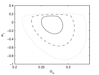
Figure 1: The $1\sigma$ (solid line), $2\sigma$ (dashed line), and $3\sigma$ (dotted line) contour plots of $\Omega_{\textrm{m}}$-$w_{1}$ relation in model (iii).

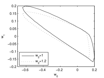
Figure 2: The $1\sigma$ contour plots of $w_{0}$-$w_{1}$ relation in model (v) showing no particular preference to quintessence or phantom.

V Conclusion and discussion

We have obtained a class of exact solutions of the tachyon field in the framework of Friedmann universe. The solutions of the Hubble parameter $H$, the scale factor $a$, and the potential $V$ are expressed by general integrations of a given generating function $F(\phi)$. We list the exact solutions of some special generating functions, such as the constant, the power-law, and the exponential functions. By the results one is tempted to postulate that the tachyon field may provide a possible explanation to the dark energy. According to the solutions of the tachyon field, we propose some parameterized EOS parameters of dark energy in the cosmological evolution, thus these tachyon-inspired dark energy models predict some new $H$-$z$ relations in cosmology. We employ the SNLS data with the parameters $\mathcal{A}$ and $\mathcal{R}$ to constrain our models. The results show that the tachyon field can be a candidate for the dark energy, and the phantom case is slightly favored to fit the SNe Ia data, though there is still no way to rule out the simplest cosmological constant as a good dark energy candidate.

In this work, the tachyon field that causes the late-time accelerating expansion of the Universe, instead of the problematic yet economic cosmological constant. The generating function method enables us to obtain exact solutions to explore the properties of the tachyon field. Furthermore, another class of scalar field, the k-essence kes has also related to the DBI action and likewise this generating function method can similarly be applied to it. Beside, other approaches are also interesting, such as in Ref. od . Currently, lots of exotic components are proposed to explain the cosmic dark components (dark matter and dark energy) and too many of them fit the data well. However, we believe that the seemingly chaotic situation would be improved as the incoming more precise data sets in observational cosmology available and we may gain some new knowledge not far away.

Appendix A A note on the mixture of dust and dark energy

If there are several components in the Universe, we can solve the Friedmann equations to obtain the Hubble parameter $H(z)$. Assuming that only the $i$th component is in the Universe, we can solve a relation $H_{i}(z)$. The question is whether the addition law $H(z)^{2}=\sum_{i}H_{i}(z)^{2}$ is correct. This is not always true in general. The reason is as follows. From Eq. (5), the equation determining the Hubble parameter is $\dot{H}=-\frac{3}{2}H^{2}+\sum_{i}\Lambda_{i}$ if there are the dust and other components $\Lambda_{i}$ in the Universe. This equation can be rewritten as

$$\frac{1}{2}(1+z)\frac{d(H^{2})}{dz}=\frac{3\gamma}{2}H^{2}-\sum_{i}\Lambda_{i}.$$ (25)

If each $\Lambda_{i}$ is only explicitly dependent on the redshift $z$ or just constant, this is an inhomogeneous linear differential equation, and $\Lambda_{i}$ are the inhomogeneous terms. According to the theory of linear differential equations, the solution of the this equation is equal to the summation of the solutions when each nonhomogeneous term exists. Therefore, the conclusion is that if the component contributes a term which is only explicitly dependent on the redshift $z$ (equally, the scale factor $a$) or constant, the addition law is correct.

For example, the curvature term is proportional to $1/a^{2}$, and the cosmological constant is a constant. Therefore, the corresponding terms of the dust, the curvature, and the cosmological constant can be added to have $H^{2}$ as a polynomial. In the case of the bulk viscosity, which contributes a term proportional to $H$ bre02 ; eos4 , even an explicit $H(z)$ relation unable to be obtained, consequently, $H^{2}$ cannot be separated to a $(1+z)^{3}$ term and a dark energy term simply. The tachyon field is far more complicated than the only $z$-dependent term, thus Eq. (20) may not exactly valid. However, since the $\Lambda$CDM model is in good agreement with the globally observational data, the behavior the dark energy should not be deviated from the cosmological constant too far away. It is reasonable to assume that the addition law is valid for the mixture of the dust and dark energy as an approximation, as that is correct for the limit case to the cosmological constant.

References

- (1) A. G. Riess et al., Astron. J. 116, 1009 (1998); N. Bahcall, J. P. Ostriker, S. Perlmutter, and P. J. Steinhardt, Science 284, 1481 (1999); A. G. Riess et al., astro-ph/0611572.
- (2) C. L. Bennett et al., Astrophys. J. Suppl. 148, 1 (2003); D. N. Spergel et al., astro-ph/0603449.
- (3) P. Astier et al., Astron. Astrophys. 447, 31, (2006), astro-ph/0510447.
- (4) S. Weinberg, Rev. Mod. Phys.61, 1 (1989)
- (5) S. Nojiri and S. D. Odintsov, Phys. Rev. D 72, 023003 (2005), hep-th/0505215.
- (6) S. Capozziello, V. F. Cardone, E. Elizalde, S. Nojiri, and S. D. Odintsov, Phys. Rev. D 73, 043512 (2006), astro-ph/0508350.
- (7) S. Capozziello, S. Nojiri, and S. D. Odintsov, Phys. Lett. B 634, 93 (2006), hep-th/0512118.
- (8) J. Ren and X. H. Meng, Phys. Lett. B 633, 1 (2006), astro-ph/0511163; 636, 5 (2006), astro-ph/0602462; Int. J. Mod. Phys D 16, 1341 (2007), astro-ph/0605010.
- (9) A. Kamenshchik, U. Moschella, and V. Pasquier, Phys. Lett. B 511, 265 (2001), gr-qc/0103004.
- (10) X. H. Meng and P. Wang, Class. Quant. Grav. 20, 4949 (2003); 21, 951 (2004); 22, 23 (2005); Gen. Rel. Grav. 36, 1947 (2004); Phys. Lett. B 584, 1 (2004); astro-ph/0308284; hep-th/0310038.
- (11) P. J. E. Peebles and B. Ratra, Rev. Mod. Phys. 75, 559 (2003), astro-ph/0207347.
- (12) T. Padmanabhan, Phys. Rept. 380, 235 (2003), hep-th/0212290.
- (13) A. A. Sen, I. Chakrabarty, and T. R. Seshadri, Gen. Rel. Grav. 34, 477 (2002), gr-qc/0005104.
- (14) L. P Chimento, V. Méndez, and N. Zuccalá, Class. Quantum Grav. 16, 3749 (1999).
- (15) A. Sen, JHEP 0204, 048 (2002), hep-th/0203211; JHEP 0207, 065 (2002), hep-th/0203265; Mod. Phys. Lett. A 17, 1797 (2002), hep-th/0204143.
- (16) J. S. Bagla, H. K. Jassal, and T. Padmanabhan, Phys. Rev. D 67, 063504 (2003), astro-ph/0212198.
- (17) G. Shiu and I. Wasserman, Phys. Lett. B 541, 6 (2002), hep-th/0205003; G. Shiu, S.-H. H. Tye, Ira Wasserman, Phys. Rev. D 67, 083517 (2003), hep-th/0207119.
- (18) P. F. Gonzalez-Diaz, Phys. Rev. D 70 063530 (2004), astro-ph/0408450.
- (19) E. J. Copeland, M. R. Garousi, M. Sami, and S. Tsujikawa, Phys. Rev. D 71 043003 (2005), hep-th/0411192.
- (20) S. Panda, M. Sami, and S. Tsujikawa, Phys. Rev. D 73, 023515 (2006), hep-th/0510112.
- (21) A. de la Macorra, U. Filobello, G. German, Phys. Lett. B 635 (2006) 355 (2006), hep-th/0601052.
- (22) G. Calcagni and A. R. Liddle, Phys. Rev. D 74, 043528 (2006), astro-ph/0606003.
- (23) M. B. Causse, astro-ph/0312206; S. K. Srivastava, gr-qc/0409074; gr-qc/0411088; T. Kobayashi, gr-qc/0608104; Y. Shao and Y. Gui, gr-qc/0703111; gr-qc/0703112.
- (24) R. R. Caldwell, Phys. Lett. B 545, 23 (2002), astro-ph/9908168.
- (25) R. R. Caldwell, M. Kamionkowski, and N. N. Weinberg, Phys. Rev. Lett. 91, 071301 (2003), astro-ph/0302506.
- (26) J. G. Hao and X. Z. Li, Phys. Rev. D 68, 043501 (2003), hep-th/0305207; Phys. Rev. D 68, 083514 (2003), hep-th/0306033.
- (27) B. Gumjudpai, T. Naskar, M. Sami, and S. Tsujikawa, JCAP 0506, 007 (2005), hep-th/0502191.
- (28) S. Nojiri and S. D. Odintsov, Phys. Lett. B 571, 1 (2003), hep-th/0306212.
- (29) W. H. Kinney and K. Tzirakis, arXiv:0712.2043 [astro-ph].
- (30) J. Martin and M. Yamaguchi, arXiv:0801.3375 [hep-th].
- (31) T. Padmanabhan, Phys. Rev. D 66 021301 (2002), hep-th/0204150.
- (32) L. R. W. Abramo and F. Finelli, Phys. Lett. B 575, 165 (2003), astro-ph/0307208.
- (33) S. Nojiri, S. D. Odintsov, and S. Tsujikawa, Phys. Rev. D 71, 063004 (2005), hep-th/0501025.
- (34) M. C. Bento, O. Bertolami, N. M. C. Santos, and A. A. Sen, Phys. Rev. D 71, 063501 (2005); Y. Gong and Y. Z. Zhang, Phys. Rev. D 72, 043518 (2005); X. Zhang and F. Q. Wu, Phys. Rev. D 72, 043524 (2005); X. Zhang, F. Q. Wu, and J. Zhang, JCAP 0601, 003 (2006); astro-ph/0701405.
- (35) D. J. Eisenstein et al., Astrophys. J. 633 (2005) 560, astro-ph/0501171.
- (36) Y. Wang and P. Mukherjee, Astrophys. J. 606 (2004) 654, astro-ph/0312192; Y. Wang and M. Tegmark, Phys. Rev. Lett. 92 (2004) 241302, astro-ph/0403292.
- (37) L. P. Chimento, Phys. Rev. D 69, 123517 (2004), astro-ph/0311613.
- (38) S. Nojiri, S. D. Odintsov, and H. Stefancic, Phys. Rev. D 74, 086009 (2006), hep-th/0608168; S. Nojiri and S. D. Odintsov, Phys. Rev. D 74, 086005 (2006), hep-th/0608008; Phys. Lett. B 639, 144 (2006), hep-th/0606025.
- (39) I. Brevik, Phys. Rev. D 65, 127302 (2002), gr-qc/0204021.