Constraints on Reionization and Source Properties from the Absorption Spectra of $z>6.2$ Quasars

Abstract

We make use of hydrodynamical simulations of the intergalactic medium (IGM) to create model quasar absorption spectra. We compare these model spectra with the observed Keck spectra of three $z>6.2$ quasars with full Gunn-Peterson troughs: SDSS J1148+5251 ($z=6.42$), SDSS J1030+0524 ($z=6.28$), and SDSS J1623+3112 ($z=6.22$). We fit the probability density distributions (PDFs) of the observed Lyman $\alpha$ optical depths ($\tau_{\alpha}$) with those generated from the simulation, by adopting a template for the quasar’s intrinsic spectral shape, and exploring a range of values for the size of the quasar’s surrounding HII region, $R_{S}$, the volume-weighted mean neutral hydrogen fraction in the ambient IGM, $\bar{x}_{\rm HI}$, and the quasar’s ionizing photon emissivity, $\dot{N}_{Q}$. In order to avoid averaging over possibly large sightline–to–sightline fluctuations in IGM properties, we analyze each observed quasar independently. We find the following results for J1148+5251, J1030+0524, and J1623+3112: The best–fit sizes $R_{S}$ are 40, 41, and 29 (comoving) Mpc, respectively. For the later two quasars, the value is significantly larger than the radius corresponding to the wavelength at which the quasar’s flux vanishes. These constraints are tight, with only $\sim 10\%$ uncertainties, comparable to those caused by redshift–determination errors. The best–fit values of $\dot{N}_{Q}$ are 2.1, 1.3, and 0.9 $\times$ 10⁵⁷ s^-1, respectively, with a factor of $\sim$ 2 uncertainty in each case. These values are a factor of $\sim$ 5 lower than expected from the template spectrum of Telfer et al. (2002). Finally, the best–fit values of $\bar{x}_{\rm HI}$ are 0.16, 1.0, and 1.0, respectively. The uncertainty in the case of J1148+5251 is large, and $\bar{x}_{\rm HI}$ is not well constrained. However, for both J1030+0524 and J1623+3112  we find a significant lower limit of $\bar{x}_{\rm HI}\mathrel{\hbox to0.0pt{\lower 4.0pt\hbox{\hskip 1.0pt$\sim$}\hss}\raise 1.0pt\hbox{$>$}}0.033$. Our method is different from previous analyses of the GP absorption spectra of these quasars, and our results strengthen the evidence that the rapid end–stage of reionization is occurring near $z\sim 6$.

1. Introduction

The epoch of reionization, when the radiation from early generations of astrophysical objects ionized the intergalactic medium (IGM), offers a wealth of information about cosmological structure formation and physical processes in the early universe. Only recently have we begun to gather clues concerning this epoch. The Thomson scattering optical depth, $\tau_{e}=0.09\pm 0.03$ (Page et al., 2006; Spergel et al., 2006b), measured from the polarization anisotropies in the cosmic microwave background (CMB) by the Wilkenson Microwave Anisotropy Probe (WMAP), suggests that cosmic reionization began at redshift $z\mathrel{\hbox to0.0pt{\lower 4.0pt\hbox{\hskip 1.0pt$\sim$}\hss}\raise 1.0pt\hbox{$>$}}10$. However, the current uncertainty of this value, and the fact that the optical depth measures only an integrated electron column density, means that many possible competing reionization scenarios can still be accommodated.

In order to chart the progress of reionization, several attempts have been made to measure the neutral fraction of the IGM at high redshifts ($z\mathrel{\hbox to0.0pt{\lower 4.0pt\hbox{\hskip 1.0pt$\sim$}\hss}\raise 1.0pt\hbox{$>$}}6$). The detection of dark spectral regions, so-called Gunn-Peterson (GP) troughs, in the Lyman line absorption spectra of high-redshift quasars discovered in the Sloan Digital Sky Survey (SDSS) offers a probe of the late stages of reionization. The Ly$\alpha$ optical depths associated with such GP troughs, and more importantly their accelerated evolution at $z\mathrel{\hbox to0.0pt{\lower 4.0pt\hbox{\hskip 1.0pt$\sim$}\hss}\raise 1.0pt\hbox{$>$}}6$, suggests that the reionization epoch is ending at $z\sim 6$, with a lower limit on the volume-weighted IGM neutral fraction, $\bar{x}_{\rm HI}(z\sim 6)\mathrel{\hbox to0.0pt{\lower 4.0pt\hbox{\hskip 1.0pt$\sim$}\hss}\raise 1.0pt\hbox{$>$}}10^{-3}$, along at least the line of sight (LOS) to two quasars (White et al., 2003; Fan et al., 2006a). The sharp decline in flux at the edge of the GP trough of quasar J1030+0524 can be used to infer the stronger constraint of $\bar{x}_{\rm HI}(z\sim 6)\mathrel{\hbox to0.0pt{\lower 4.0pt\hbox{\hskip 1.0pt$\sim$}\hss}\raise 1.0pt\hbox{$>$}}0.2$, along that LOS (Mesinger & Haiman, 2004). The observed size of the quasars’ surrounding HII regions can be used to infer a similar, independent lower limit (Wyithe & Loeb, 2004; Mesinger & Haiman, 2004), although this requires additional assumptions concerning the quasar and its environment, and the inferred neutral fraction scales directly with these assumptions (Bolton & Haehnelt, 2006; Maselli et al., 2006). The rapid evolution in the sizes of the HII regions for different quasars between $z\sim 5.7$ and $z\sim 6.4$ suggests that the average neutral fraction increased by a factor of $\sim 10$ during this interval (Fan et al., 2006a), although there are alternative ways to account for the steep size–evolution (Bolton & Haehnelt, 2006). The distribution of spectral sizes of dark gaps should help distinguish these scenarios in the future (Gallerani et al., 2006; Fan et al., 2006a). Upper limits on the neutral fraction at $z\sim 6$ have also been suggested by other means. The lack of significant evolution in the luminosity function (LF) of Lyman $\alpha$ emitters between $z\approx 5.7$ and $z\approx 6.5$ was used to infer $\bar{x}_{\rm HI}(z\sim 6)\mathrel{\hbox to0.0pt{\lower 4.0pt\hbox{\hskip 1.0pt$\sim$}\hss}\raise 1.0pt\hbox{$<$}}0.3$ (Malhotra & Rhoads, 2004; Haiman & Cen, 2005), if the galaxies are assumed to lie in isolation, or $\bar{x}_{\rm HI}(z\sim 6)\mathrel{\hbox to0.0pt{\lower 4.0pt\hbox{\hskip 1.0pt$\sim$}\hss}\raise 1.0pt\hbox{$<$}}0.5$ (Furlanetto et al., 2006), if an analytic prescription of the clustering of HII bubbles (Furlanetto et al., 2004b) is taken into account. However, a recent, more accurate measurement of the LF at $z\approx 6.5$ revealed evidence of a decrease, weakening these upper limits (Kashikawa et al., 2006). Finally, the lack of noticeable absorption due to the Ly$\alpha$ damping wing in the afterglow spectrum of the gamma-ray burst 050904 at $z=6.3$ can constrain $\bar{x}_{\rm HI}(z\sim 6)\mathrel{\hbox to0.0pt{\lower 4.0pt\hbox{\hskip 1.0pt$\sim$}\hss}\raise 1.0pt\hbox{$<$}}0.2$ along that LOS (Totani et al., 2006).

The preponderance of constraints mentioned above suggests that the combination of all existing data is consistent with $\bar{x}_{\rm HI}(z\sim 6)\sim 0.1$. While this is plausible, the constraints listed above all rely on various model assumptions. For example, the conversion of an observed average flux decrement to a neutral fraction (Fan et al., 2002; White et al., 2003; Fan et al., 2006a) is difficult, and requires precise ab–initio knowledge of the IGM density distribution at high-redshifts (Oh & Furlanetto, 2005; Fan et al., 2006a). All of the other constraints mentioned above rely on the IGM density distribution, as well, albeit less sensitively. Techniques involving the sizes of HII regions (Wyithe & Loeb, 2004; Maselli et al., 2006; Fan et al., 2006a) are subject to degeneracies between quasar lifetime, ionizing flux, and the IGM neutral fraction. Further complicating matters for the HII bubble size techniques is the fact that the onset of the GP trough need not correspond to the edge of the HII region. The GP through just corresponds to the region where the flux drops below the detection threshold, and thus merely provides a lower limit on the size of the HII region (Mesinger & Haiman 2004; Maselli et al. 2006; see also Bolton & Haehnelt 2006 for a recent, comprehensive review of these issues). Furthermore, determining the number density and evolution of Ly$\alpha$ emitting galaxies is complicated and depends on knowledge of galaxy clustering (Haiman & Cen, 2005; Furlanetto et al., 2004a, 2006), absorber clustering, as well as the large-scale density (e.g. Barkana & Loeb 2004b, a) and velocity fields (e.g. Cen et al. 2005), which are all unconstrained at the relevant high redshifts.

More generally, the drawback of many of these methods is that they rely on the combination of data from multiple LOSs to obtain statistical significance. However, assuming constancy in the IGM properties along disparate LOSs is dangerous at high-redshifts, especially approaching the end of reionization, when large sightline-to-sightline fluctuations are expected in the density field and the ionizing background (see, e.g., recent reviews by Djorgovski et al. 2006 and Lidz et al. 2006). Indeed, the current sample of high-redshift quasars already reveals large fluctuations in the IGM properties along different LOSs (Fan et al., 2006a). This would suggest that the most rewarding technique would be able to analyze and obtain constraints from each source independently from other sources. This is statistically less powerful (e.g. Mesinger et al. 2004), but the rewards can be rich, potentially providing additional constraints on the properties of individual quasars and their environments, such as the quasar’s emissivity of ionizing photons, size of its surrounding HII region, sharpness of the HII region boundary, the quasars’ X-ray emission, as well as a measure of the sightline-to-sightline fluctuations in these quantities (Mesinger & Haiman, 2004).

The purpose of this paper is to derive these parameters, i.e. the hydrogen neutral fraction, the size of surrounding HII region, and the ionizing emissivity, by separately modeling the spectra of each of the $z>6.2$ quasars. Specifically, we analyze J1148+5251 ($z=6.42$), J1030+0524 ($z=6.28$) and J1623+3112 ($z=6.22$). At present, a 4th quasar is known with a full GP trough. This source, however, is a broad absorption line (BAL) quasar J1048+4637 ($z=6.2$), with complex spectral features (Fan, X., private communication) that preclude a simple interpretation in terms of IGM properties. We have therefore omitted this quasar from our study.

Our analysis differs from our previous work (Mesinger & Haiman, 2004) where we modeled the gross transmission features in Ly$\alpha$ and Ly$\beta$ close to the edge of the HII region surrounding J1030+0524. In the present study, we perform a much more detailed analysis, by fitting the quasar’s intrinsic emission, and modeling the distribution of optical depths, pixel–by–pixel, blueward of the Ly$\alpha$ line center, following the procedure proposed in Mesinger et al. (2004). Unlike in Mesinger & Haiman (2004), here we do not make use of the Ly$\beta$ absorption spectrum, except to set a lower limit in the allowed size of the HII region surrounding J1030+0524, the only one among the three quasars that has a noticeable offset between the Ly$\alpha$ and Ly$\beta$ GP troughs. Our reason for ignoring the Ly$\beta$ region is that the majority of the pixels we analyze (see Figure 2 below) have flux detected in the Ly$\alpha$ absorption region, which can directly be converted to a Ly$\alpha$ optical depth. This avoids the need for a statistical modeling of the foreground Ly$\alpha$ absorption, necessary to convert Ly$\beta$ to a Ly$\alpha$ optical depth.

This paper is organized as follows. In § 2, we describe our analysis technique, including generating the simulated absorption (§ 2.1), fitting for the quasars’ intrinsic emission spectrum (§ 2.2), and the statistical method used to compare the observed and simulated spectra (§ 2.3). In § 3, we present our results for each of the quasars we analyze. In § 4, we discuss various aspects of our results, such as the origin of the constraints we obtain, and the robustness of our results in the face of uncertainties in the quasar template spectrum. In § 5, we summarize our key findings and present our conclusions.

2. Analysis

In this section, we describe the three components of our analysis: (i) a hydrodynamical simulation to model the absorption (§ 2.1); (ii) modeling the quasars’ intrinsic emission spectrum (§ 2.2); and (iii) the statistical comparison of observed and simulated spectra (§ 2.3). Unless stated otherwise, we adopt the background cosmological parameters ($\Omega_{\Lambda}$, $\Omega_{\rm M}$, $\Omega_{b}$, n, $\sigma_{8}$, $H_{0}$) = (0.76, 0.24, 0.0407, 1, 0.76, 72 km s^-1 Mpc^-1), consistent with the three–year results by the WMAP satellite (Spergel et al., 2006a). We use redshift, $z$, and the observed wavelength, $\lambda_{\rm obs}$, interchangeably throughout this paper as a measure of the distance along the line of sight. Unless stated otherwise, we quote all quantities in comoving units.

2.1. Simulating Absorption in the IGM

In order to simulate the absorption spectra, we make use of a hydrodynamical simulation box in a $\Lambda$CDM universe at redshift $z$ = 6. The details of the simulation are described in Cen et al. (2003), and we only briefly discuss the relevant parameters here. The box is 11 $h^{-1}$ Mpc on each side, with each pixel being about 25.5 $h^{-1}$ kpc. This scale resolves the Jeans length in the smooth, partially-ionized IGM by more then a factor of 10. The box also has a slightly different set of cosmological parameters: $(\Omega_{\Lambda},\Omega_{M},\Omega_{b},n,\sigma_{8},$ $H_{0})$ = (0.71, 0.29, 0.047, 1, 0.85 , 70 km s^-1 Mpc^-1).

Density and velocity information was extracted from the simulation box along randomly chosen lines of sight. The step size along each LOS was taken to be 5.1 $h^{-1}$ kpc, which resolves the Lyman $\alpha$ Doppler width in the partially-ionized IGM by more than a factor of 40. The exact value of the step size was chosen somewhat arbitrarily, and does not influence the results as long as it adequately resolves the Doppler width. At each step, the density and velocity values were averaged for the neighboring pixels, and weighted by the distance to the center of the pixels. We extended each LOS by the common practice of randomly choosing a LOS through the box, and stacking several segments together (Cen, 1994; Mesinger et al., 2004; Kohler et al., 2005; Bolton & Haehnelt, 2006). The r.m.s. mass fluctuation on the scale the box is $\sigma(z=6.3)\sim 0.15$. This is a small enough value that neglecting wavelengths longer than the box size is justified in our analysis. Note however, that this is not the case for modeling highly non-linear processes, such as reionization (e.g. Barkana & Loeb 2004b). When using such a LOS in simulating a given quasar spectrum, density values from the simulation were scaled as $(1+z)^{3}$.

The total optical depth due to Lyman $\alpha$ absorption, $\tau$, between an observer at z = 0 and a source at z = $z_{\rm Q}$, at an observed wavelength of $\lambda_{\rm obs}=\lambda_{0}(1+z_{\rm Q})$, is given by:

$$\tau(\lambda_{\rm obs})=\int_{0}^{z_{\rm Q}}dz~{}c\frac{dt}{dz}~{}n(z)~{}x_{\rm HI}(z)~{}\sigma\left[\frac{\lambda_{\rm obs}}{(1+z)(1-\frac{v(z)}{c})}\right]$$ (1)

where $n(z)$, $v(z)$, $x_{\rm HI}(z)$ are the total hydrogen number density, the component of the peculiar velocity along the LOS, and the local hydrogen neutral fraction, respectively, at redshift $z$. The Ly$\alpha$ absorption cross section, to first order in $v(z)/c$, is given by $\sigma[\lambda_{\rm obs}/(1+z)/(1-v(z)/c)]$.

Since high-redshift quasars are surrounded by their own highly ionized HII regions, it is useful to express $\tau$ as a sum of contributions from inside ($\tau_{R}$) and outside ($\tau_{D}$) the HII region, $\tau=\tau_{R}+\tau_{D}$. Defined as such, the resonant optical depth, $\tau_{R}$, would be given by Eq. (1), with the lower limit of integration changed to the redshift corresponding to the edge of the HII region, $z(R_{S})$. The damping wing optical depth $\tau_{D}$, would be given by Eq. (1), with the upper limit of integration changed to $z(R_{S})$ .

Since cosmic hydrogen is highly ionized at low redshifts, one can replace the lower limit of integration in Eq. (1) with $z_{\rm end}$, denoting the redshift below which HI absorption becomes insignificant along the LOS to the source. In our analysis, we chose the value of $z_{\rm end}$ separately for each quasar to correspond approximately to the blue edge of its GP trough. This roughly translates to $z_{\rm end}\sim$ 0.2–0.3 for our three quasars. We find that the exact choice of $z_{\rm end}$ is not important, because most of the contribution to $\tau_{D}$ comes from neutral hydrogen close to $z(R_{S})$. Inside the HII region, we assume an IGM temperature of $T=2\times 10^{4}$ K. Outside the HII region, for the case of a mostly ionized universe, we assume an IGM temperature of $T=10^{4}$ K, while the temperature in a neutral universe was taken to be $T=2.73\times 151(\frac{1+z}{151})^{2}$ K, valid for $z<150$ (Peebles, 1993). Our results are fairly insensitive to the exact temperature used. The Doppler width of the Lyman-$\alpha$ absorption cross section scales as $\nu_{D}\propto T^{1/2}$, but the total integrated area under the cross section is independent of temperature.

Assuming ionization equilibrium, we compute the neutral hydrogen fraction at each point along the LOS with:

$$nx_{\rm HI}(\Gamma_{\rm Q}+\Gamma_{\rm BG})=n^{2}(1-x_{\rm HI})^{2}\alpha_{B}~{},$$ (2)

where $\Gamma_{\rm Q}$ and $\Gamma_{\rm BG}$ are the number of ionizations per second per hydrogen atom due to the quasar’s and the background’s ionizing fluxes, respectively, and $\alpha_{B}$ is the case-B hydrogen recombination coefficient. The LHS of Eq. (2) accounts for the number of hydrogen ionizations per cm³, while the RHS accounts for the number of hydrogen recombinations per cm³. Solving Eq. (2) for $x_{\rm HI}$ one obtains:

$$x_{\rm HI}=\frac{-b-\sqrt{b^{2}-4}}{2}~{},$$ (3)

where $b\equiv-2-(\Gamma_{\rm Q}+\Gamma_{\rm BG})/(n\alpha_{B})$. We further parametrize the quasar’s ionization rate with:

$$\Gamma_{\rm Q}\equiv f_{\Gamma}\Gamma^{e}_{\rm Q}$$ (4)

where $\Gamma^{e}_{\rm Q}=(4\pi r^{2})^{-1}\int_{\nu_{H}}^{\infty}1.55\times 10^{31}$ $(\nu/\nu_{H})^{-1.8}$ $[(1+z)/(1+z_{\rm Q})]^{-0.8}(\sigma/h\nu)d\nu$ s^-1, with $\nu_{H}=3.29\times 10^{15}$ Hz being the ionization frequency of hydrogen and $r$ being the luminosity distance between the source and redshift $z$. $\Gamma^{e}_{\rm Q}$ results from redshifting a power–law spectrum with a slope of $\nu^{-1.8}$, normalized such that the emission rate of ionizing photons per second is $1.3\times 10^{57}$, matching the emissivity one obtains (Haiman & Cen, 2002) for SDSS J1030+0524 using a standard template spectrum (Elvis et al., 1994). Note that the normalization inferred from the more recent template of Telfer et al. (2002) is a factor of of $\sim 5$ higher. This roughly translates to an emission rate of ionizing photons of

$$\dot{N}_{Q}=f_{\Gamma}\times 1.3\times 10^{57}~{}{\rm s^{-1}}~{}.$$ (5)

We ignore radiative transfer along the LOS (and also the ionization of helium). Instead, outside of the quasar’s HII region, we compute $x_{\rm HI}$ assuming the quasar contributes nothing to the ionizing flux, i.e. $\Gamma_{\rm Q}(R>R_{S})=0$, while inside the HII region, we assume the gas is optically thin in the ionizing continuum. This assumption of a sharp HII region boundary is an approximation, valid in the regime where either the quasar’s spectrum is soft, or where a strong soft ionizing background flux dominates over that of the quasar already at radii smaller that the mean free path of the typical ionizing quasar photon (as is the case of the proximity effect at lower redshift; Bajtlik et al. 1988) If the quasar has a hard spectrum, and the background intensity is low, then the edge of the HII region will be “blurred”. A similar blurring would arise if additional ionizing sources inside the HII region, with an extended spatial distribution, would contribute significant flux (Wyithe & Loeb, 2006), a possibility we do not address here. However, already strong upper limits can be placed on the extent of such blurring from the offset between the wavelengths of the Ly$\alpha$ and Ly$\beta$ GP troughs. Since Ly$\beta$ absorption is less sensitive than Ly$\alpha$, the amount of offset between the GP troughs gives a measure of the spatial (i.e. wavelength) evolution of $\tau$ close to the edge of the HII region, with a large offset indicating slow $\tau$ evolution, and a small offset indication rapid $\tau$ evolution. Mesinger & Haiman (2004) studied this for the case of J1030+0524, but even stronger constraints could be placed on the spectra of J1148+5251 and J1623+3112, since they do not show any offsets between the GP troughs (Kramer et al., in preparation). Furhtermore, neglecting possible obscuration effects arising from optically thick gas and dust close to the quasar can bias our determination of the quasar’s luminosity to lower values. This means that our determination of the quasar’s luminosity should be viewed as the observed luminosity along the LOS, and equal to the intrinsic luminosity in the low opacity limit.

Finally, we define the neutral hydrogen fraction in the IGM, $x_{\rm HI}^{\rm IGM}$, with Eq. (3) using the mean density of the universe at the edge of the HII region, $n=n_{0}[1+z(R_{S})]^{3}$, and $\Gamma_{\rm Q}=0$. Although $\Gamma_{\rm BG}$ is the more physically relevant quantity and we use it in our analysis, henceforth we will use $x_{\rm HI}^{\rm IGM}$ as the proxy for $\Gamma_{\rm BG}$ in order to match convention. As defined above, $x_{\rm HI}^{\rm IGM}$ represents the neutral fraction at the mean density. The more common representation of the neutral fraction in the literature is in the form of the volume (or mass) weighted mean, $\bar{x}_{\rm HI}$. This definition, of course, depends on the assumed density distribution. Hence, for comparison purposes, we express our results both in terms of $x_{\rm HI}^{\rm IGM}$ and $\bar{x}_{\rm HI}$, with the latter obtained by averaging over our simulation box densities and assuming ionization equilibrium.

To summarize, our analysis has three free parameters:

1. $R_{S}$, the radius of the quasar’s HII region,

2. $x_{\rm HI}^{\rm IGM}$, the neutral hydrogen fraction in the IGM at mean density,

3. $f_{\Gamma}$, the quasar’s ionizing luminosity, in units of $1.3\times 10^{57}~{}{\rm s^{-1}}$.

To obtain an intuition for the effect of varying these free parameters, in Figure 1 we plot $\tau_{R}$ (solid curve) and $\tau_{D}$ (dashed curve) for a typical simulated LOS, for parameter choices ($R_{S}$, $x_{\rm HI}^{\rm IGM}$, $f_{\Gamma}$) = (40 Mpc, 1, 1). As stated above, the total Lyman $\alpha$ optical depth is the sum of these two contributions, $\tau$ = $\tau_{R}$ + $\tau_{D}$. Roughly speaking, changing $R_{S}$ moves the dashed ($\tau_{D}$) curve left and right, while changing $x_{\rm HI}^{\rm IGM}$ moves this curve up and down in Figure 1. Changing $f_{\Gamma}$ approximately corresponds to moving the solid ($\tau_{R}$) curve up and down. The dotted line demarcates roughly the maximum total optical depth, $\tau\sim 5.5$, at which a signal can be detected with a confidence greater than 1-$\sigma$, in the spectral region just blueward of the Ly$\alpha$ emission line (see discussion in § 2.3). Finally, after the optical depth and the associated transmission ($e^{-\tau}$) is calculated according to the procedure outlined above, the transmission is averaged over $\approx$ 3.3 Å wavelength bins to match the Keck ESI spectra with which the simulated spectra are compared (note that the actual smoothing length $\Delta\lambda_{\rm obs}$ differs by a few percent for each source, since they are at different redshifts).

                                                                        

Figure 1.— Model from a hydrodynamical simulation for the optical depth contributions from within ($\tau_{R}$) and from outside ($\tau_{D}$) the local ionized region for a typical line of sight towards a $z_{\rm Q}=6.42$ quasar. This figure was created with parameter choices ($R_{S}$, $x_{\rm HI}^{\rm IGM}$, $f_{\Gamma}$) = (40 Mpc, 1, 1). The dashed curve corresponds to $\tau_{D}$, and the solid curve corresponds to $\tau_{R}$. The total Lyman $\alpha$ optical depth is the sum of these two contributions, $\tau$ = $\tau_{R}$ + $\tau_{D}$. The dotted line demarcates roughly the maximum total optical depth, $\tau\sim 5.5$, at which a signal can be detected with a confidence greater than 1-$\sigma$, in the spectral region just blueward of the Ly$\alpha$ emission line (see discussion in § 2.3). In our analysis, the transmission ($e^{-\tau}$) is averaged over $\sim$ 3 – 4 Å wavelength bins (1/10 of the resolution in the figure above), thus decreasing the fluctuation in the effective optical depth. For reference, the redshifted Ly$\alpha$ wavelength is at 9020 Å, off the plot.

The free parameter $R_{S}$ was varied in linear increments of $\Delta R_{S}=2$ Mpc, with the lower limit set by the red edge of the Ly$\alpha$ GP through in the observed spectra. The other parameters were varied in the ranges: $3.2\times 10^{-4}\leq x_{\rm HI}^{\rm IGM}\leq 1$, in multiples of 5, and $0.1\leq f_{\Gamma}\leq 10$, in linear increments of $\Delta f_{\Gamma}=0.3$ between $0.1\leq f_{\Gamma}\leq 2$ and $\Delta f_{\Gamma}=2$ between $2<f_{\Gamma}\leq 10$.

2.2. Modeling the Intrinsic Emission Spectrum

As observational input in our analysis, we make use of Keck ESI spectra of the three highest redshift quasars discovered to date: J1148+5251 ($z_{\rm Q}=6.42$), J1030+0524 ($z_{\rm Q}=6.28$), and J1623+3112 ($z_{\rm Q}=6.22$). These quasars are the only quasars discovered to date with $z_{\rm Q}>6.2$, as well as the only quasars (aside from the BAL quasar J1048+4637) exhibiting complete GP troughs, with no detectable flux over a wide wavelength range (Fan et al., 2006b). Readers interested in the details of the corresponding observations are encouraged to consult Fan et al. (2006b) and White et al. (2003).

In order to compare the quasars’ observed spectra with our simulated spectra, we must know the intrinsic emission spectrum from each of the observed sources. Observations of lower redshift quasars (e.g. Telfer et al. 2002) suggest that their intrinsic continuum emission is well fit by a broken power–law, with a mean spectral slope of $\alpha\sim-0.7$ ($f_{\nu}\propto\nu^{\alpha}$) redward of the Ly$\alpha$ line, and a slope of $\alpha\sim-1.8$ blueward of the Ly$\alpha$ line. The high-redshift SDSS quasars do not show any evidence for deviating from this trend (e.g. White et al. 2003). The precise location of the wavelength of the break in the power–law is difficult to determine for any given source, due to a strong broad Ly$\alpha$ emission line superimposed on the continuum spectrum. However, for our purposes, we are interested in the optical depth at wavelengths within just a few tens of rest-frame Angstroms blueward of the Ly$\alpha$ line center, where the Ly$\alpha$ emission line is still dominant over the continuum. Therefore, we do not model the break, and use a single power–law continuum component instead in our emission template. Throughout our analysis, we keep the logarithmic slope $\alpha=-0.7$ fixed (as we will demonstrate below, our results are insensitive to this choice).

We derive our constraints below entirely from the blue side of the Ly$\alpha$ line in our analysis, where the effects of the IGM can be felt most strongly (Mesinger et al., 2004). To this end, we make use of “clean” spectral regions on the red side of the Ly$\alpha$ line, where the resonant attenuation is negligible ($\tau_{R}\sim 0$), and the damping wing attenuation is less than 10% ($e^{-\tau_{D}}>0.9$) even in the case of a fully neutral IGM and a small $R_{S}$. We fit the NV emission line at $(1+z_{\rm Q})1240.81$ Å with a single gaussian, and the continuum with a single power–law. Additionally, we fit the Ly$\alpha$ line with a single gaussian for J1148+5251 (with a fitted width of $\Delta\lambda_{\rm obs}=113$Å) and J1623+3112 (with a fitted width of $\Delta\lambda_{\rm obs}=81$Å) and with a sum of two independent gaussians for J1030+0524 (with fitted widths of $\Delta\lambda_{\rm obs}=45$Å and $\Delta\lambda_{\rm obs}=113$Å). We have found that adding a second gaussian does not improve the fits to the Ly$\alpha$ line of J1148+5251 and J1623+3112. However, the Ly$\alpha$ line of J1030+0524 requires two gaussians for an accurate fit, as it contains a broad and narrow component, similar to the shape of a Voigt profile (Ho et al., 1997; Greene & Ho, 2004). The redshifted line centers of the gaussians were held fixed in the fitting procedure, set to $(1+z_{\rm Q})\lambda_{0}$, where $\lambda_{0}=1215.67$Å for Ly$\alpha$ and $\lambda_{0}=1240.81$Å for N V. The height and width of the gaussians were then found by fitting the flux in pixels on the red side of the line center. Care was taken, in addition, to excise the spectral region immediately redward of the Ly$\alpha$ line center, as this region could be susceptible to non-negligible absorption by dense infalling gas in the foreground, close to the quasar (e.g. Mesinger et al. 2004; Barkana & Loeb 2004a). Indeed, the quasar spectra do exhibit sharp drops in the observed flux as one approaches the line center from the red side (see Fig. 2; see also Barkana & Loeb 2003). This region was excised by eye from the fitting procedure. The amplitude of the continuum was found separately, by fitting the flux in regions of the spectrum further to the red, that are a-priori known not to suffer metal line absorption, corresponding to roughly 1300 – 1350 Å in the rest frame. We explicitly avoid spectral sub–regions with obvious emission or absorption lines. More specifically, the spectral regions in the observed frame used in the fit for the continuum were (demarcated with horizontal lines in Figure 2):

• J1148+5251: 9100–9125Å, 9128–9190Å, 9220–9500Å, 9700–10000Å;

• J1030+0524: 8880–8990Å, 9020–9100Å, 9840–9930Å, 9960–10020Å;

• J1623+3112: 8830–8895Å, 8980–9040Å, 9790–9863Å, 9880–9907Å;

In Figure 2, we show the data for the observed spectra, $F(\lambda_{\rm obs})$, with 1-$\sigma$ error bars as well as the continuum + Ly$\alpha$ + N V fit to the intrinsic emission, $F_{0}(\lambda_{\rm obs})$, generated by our procedure (solid curve). The Ly$\alpha$ optical depth can then be inferred in each pixel separately as: $\tau_{\rm obs}(\lambda_{\rm obs})=-\ln[F(\lambda_{\rm obs})/F_{0}(\lambda_{\rm obs})]$.

Figure 2.— Observed spectra (shown as points with 1-$\sigma$ error bars) and the continuum + Ly$\alpha$ + N V fit of the intrinsic emission spectrum generated by our procedure (solid curve). The spectral regions (on the red side of the Ly$\alpha$ line center) that we used in the fit are marked with horizontal lines. The inlaid panels zoom in on the spectral region (on the blue side of the Ly$\alpha$ line center) that were then used to compare the absorption optical depth $\tau$ with hydrodynamical simulations. The vertical dashed lines bracket the wavelength ranges used to construct $\tau$ histograms (see § 2.3). The spectra shown are those of J1148+5251, J1030+0524, J1623+3112 (left to right).

2.3. Comparing Simulated and Observed Spectra

After the observed optical depths, $\tau_{\rm obs}(\lambda_{\rm obs})$, are obtained as discussed in § 2.2, and the simulated optical depths, $\tau_{\rm sim}(\lambda_{\rm obs})$, are obtained for every LOS and point in our parameter space as discussed in § 2.1, we wish to statistically compare the simulated and observed optical depths for each quasar. More precisely, for each quasar and every point in our three–dimensional parameter space, ($R_{S}$, $x_{\rm HI}^{\rm IGM}$, $f_{\Gamma}$), we want to answer the question: what is the likelihood that the list of $\tau_{\rm obs}(\lambda_{\rm obs})$ values and the list of $\tau_{\rm sim}(\lambda_{\rm obs})$ values were drawn from the same underlying probability distribution? Note that we have a fixed list of about 30 $\tau_{\rm obs}(\lambda_{\rm obs})$ values for each quasar, but we generate a different list of 3000 $\tau_{\rm sim}(\lambda_{\rm obs})$ values, combining 100 LOSs, for each choice of ($R_{S}$, $x_{\rm HI}^{\rm IGM}$, $f_{\Gamma}$).

We use the Kolmogorov-Smirnov (K-S) test (e.g. Press et al. 1992) to compare the cumulative probability distributions (CPDFs) – i.e., histograms – of $\tau_{\rm obs}(\lambda_{\rm obs})$ and $\tau_{\rm sim}(\lambda_{\rm obs})$. The usefulness of the K-S test is that it provides a figure of merit which can be directly interpreted as the likelihood that two distributions were drawn from the same underlying distribution, without the need for the ad-hoc binning of data, and the resulting loss of information, required by such methods as the $\chi^{2}$ test. The drawback of using the K-S test is that computing absolute confidence levels around our best fit values would require prohibitively expensive Monte-Carlo simulations. We caution the reader that, as a result, the relative likelihoods we quote below do not represent traditional “error–bars”.

Our statistical analysis is quite similar to that employed by Rollinde et al. (2005) to model density structure surrounding moderate redshift ($z\sim 2$) quasars. The main difference in technique is that while our present approach uses a parameterized model, Rollinde et al. (2005) fit for the intrinsic spectrum directly from the low–$\tau$ regions of the spectrum. Using simulated spectra, they show that by applying the K-S test on optical depth CPDFs, one can statistically discriminate among different models of the distance–evolution of the optical depth. In Mesinger et al. (2004), we use a similar statistical test to show that the moderate degeneracy between $R_{S}$ and $x_{\rm HI}^{\rm IGM}$ can be broken with a single spectrum, if $R_{S}$ is moderately constrained. This prior analysis did not take into account the additional constraint arising from the evolution of the CPDF with distance, as our current analysis does. Nevertheless, we caution the reader that these tests only confirm the ability to statistically recover input parameters using our statistical analysis. They do not test the validity of our model.

The optical depth CPDF should have a strong dependence on wavelength (since the gas is more highly ionized near the quasar). In principle, the information contained in this dependence could be extracted and used to further constrain model parameters. For example, one could compare the CPDFs of $\tau_{\rm obs}(\lambda_{\rm obs})$ and $\tau_{\rm sim}(\lambda_{\rm obs})$ in several wavelength bins for each quasar. Unfortunately, in practice, one also needs to have many points in each individual bin, to be able to sample the underlying distribution in that bin. In one extreme, as the wavelength bin size approaches the pixel width, the information from the wavelength dependence is fully preserved; however, only a single observed pixel is available to compare with a corresponding pixel from each LOS, rendering the use of the K-S test unreliable. The converse is true in the other extreme, where the wavelength bin size approaches the entire spectral region we analyze: the shape of the CPDF is accurately captured, but information from the wavelength–dependence is destroyed. Here we (somewhat arbitrarily) divide the spectral region of analysis into wavelength bins of width $\sim$ 25–30 Å, so that each bin contains between 6–8 pixels. The two blue–most bins were chosen bracket the edge of the GP trough in the observed spectrum. Furthermore, we remove the region 20–30 Å blueward of the line center from our analysis, corresponding to the expected mean radius of the large–scale overdense region surrounding such quasars (Barkana & Loeb, 2004a). This step was necessary, as our simulation box size is too small to contain a statistical sample (or even a single occurrence) of such large overdensities, required for their accurate modeling. The wavelength bins we use in our analysis are shown by the vertical dashed lines in the inlaid panels of Figure 2. We verify that our results are fairly insensitive to our choice of bin size, i.e. the relative K-S likelihoods between models change little with decreasing bin size.

In order to incorporate an uncertainty into our emission template, we add Gaussian-distributed, uncorrelated flux variations to each pixel in the template. We do this by regarding our fitted value of the template, $F_{0}(\lambda_{\rm obs})$, as the mean value of the true flux distribution, and the “true” emission at $\lambda_{\rm obs}$ is drawn from a Gaussian distribution around that mean, with a standard deviation $\sigma_{flux}(\lambda_{\rm obs})$. Hence, we replace every $\tau_{\rm sim}(\lambda_{\rm obs})$ value by a set of 1000 values, defined by

$$\tau_{\rm sim}^{\rm sampled}(\lambda_{\rm obs})\equiv-\ln[e^{-\tau_{\rm sim}(\lambda_{\rm obs})}\times A]~{},$$ (6)

where $A$ represents our emission uncertainty, and is drawn from a Gaussian distribution with a mean of 1, and a standard deviation of $\sigma_{flux}(\lambda_{\rm obs})/F_{0}(\lambda_{\rm obs})$. We set $\sigma_{flux}(\lambda_{\rm obs})/F_{0}(\lambda_{\rm obs})=0.3$, which corresponds approximately to the typical quasar-to-quasar scatter in the continuum level immediately redward of Lyman $\alpha$ (Vanden Berk et al., 2001). However, we have verified that our results are not sensitive to this choice. For example, in the case of J1623+3112, we find that in the range $0.1\mathrel{\hbox to0.0pt{\lower 4.0pt\hbox{\hskip 1.0pt$\sim$}\hss}\raise 1.0pt\hbox{$<$}}\sigma_{flux}(\lambda_{\rm obs})/F_{0}(\lambda_{\rm obs})\mathrel{\hbox to0.0pt{\lower 4.0pt\hbox{\hskip 1.0pt$\sim$}\hss}\raise 1.0pt\hbox{$<$}}0.5$, the peak K-S probability remains unchanged, and the confidence limits quoted below change at most by a single pixel in our parameter space.

Finally, in comparing spectra, one needs to define what one considers to be “zero flux”, as simulations have near-infinite precision and observations do not. To this end, we define a maximum allowed value of the optical depth, ${\rm MAX}[\tau]\equiv 5.5$. This approximately corresponds to a 1-$\sigma$ detection in our observed spectra at wavelengths around the edge of the GP trough, where the majority of pixels with fluxes less than this value are located (see Fig. 2). In our comparison, all values of $\tau>5.5$ are treated the same, regardless of their actual value.

To summarize, for each quasar we divide the spectral region roughly blueward of $\sim$ $(1+z_{\rm Q})\lambda_{\alpha}$–25Å and redward of $\sim$ $[1+z(R_{S})]\lambda_{\alpha}$–25Å into 3–5 bins of approximately equal wavelength width, containing 6–8 pixels each. In each bin we compare the CPDFs of $\tau_{\rm obs}(\lambda_{\rm obs})$ and $\tau_{\rm sim}^{\rm sample}(\lambda_{\rm obs})$ (the latter concatenated over 100 simulated LOSs). For every point in our 3D parameter space, these two distributions are compared via the K-S test, which produces a probability to be interpreted as the likelihood that the two distributions were drawn from the same underlying distribution. Finally, the K-S probabilities for each wavelength bin are multiplied to give a likelihood estimate for that point in the 3D parameter space.

3. Results

Our results for the likelihoods of various parameter–combinations are shown in Figure 3 for J1148+5251 (top), J1030+0524 (middle), and J1623+3112 (bottom). The cross in each case marks the point in the 3D parameter space where the likelihood peaks. In order from lighter to darker, the yellow, green, and blue squares correspond to points in our parameter space with likelihoods that are a factor of 27, 9, and 3 below the peak likelihood, respectively. Parameter combinations with likelihoods smaller than 1/27th of the peak are shown as empty squares.

Below, we will discuss each quasar in turn. However, it is encouraging to note first that the isocontours in Figure 3 behave as expected, following the moderate degeneracies in the parameters. Namely, since a stronger damping wing ($\tau_{D}$) contribution can be obtained either by increasing the neutral fraction or by decreasing the size of the HII region, the isocontours should be oriented from bottom-left to upper-right in each panel. Similarly, since a smaller ionizing flux (i.e. greater $\tau_{R}$) can roughly be compensated for in the total optical depth, $\tau_{R}+\tau_{D}$, by increasing the size of the HII region or decreasing the neutral fraction (both decrease $\tau_{D}$), the isocontours should shift monotonically from the upper–left to the bottom–right with increasing $f_{\Gamma}$. Both of these trends are evident in Figure 3. For example, the colored squares (corresponding to K-S likelihoods that are within a factor of 27 of the peak likelihood) in the middle row cover most of the displayed parameter space in the left–most panel, though there are no pixels with high likelihoods. Increasing the quasar’s ionizing flux (i.e. going through the panels from left to right), shifts the colored squares increasingly towards the bottom–right corner of the panel.

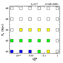
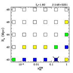
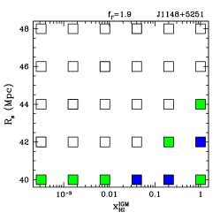
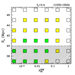
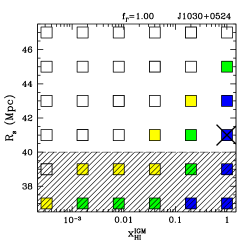
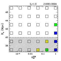
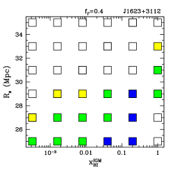
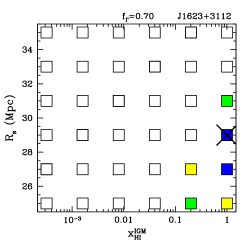
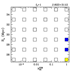
Figure 3.— Likelihoods for J1148+5251 (top), J1030+0524 (middle), and J1623+3112 (bottom) in the 3–dimensional parameter space of ($R_{S}$, $x_{\rm HI}^{\rm IGM}$, $f_{\Gamma}$). Each panel shows contours in a 2D slice of the 3D likelihood surface. The cross marks the parameter combination with the peak likelihood value (see § 2.3 for how the likelihoods were derived). In order from lighter to darker, the yellow, green, and blue squares correspond to points in our parameter space with likelihoods that are a factor of 27, 9, and 3 below the peak value, respectively. Parameter combinations with likelihoods below 1/27th of the peak are shown as empty squares. J1148+5251: The peak likelihood of 3.0% occurs at ($R_{S}$, $x_{\rm HI}^{\rm IGM}$, $f_{\Gamma}$) = (40 Mpc, 0.2, 1.6). The left, center, and right panels correspond to values of $f_{\Gamma}$= 0.7, 1.6, 1.9, respectively. J1030+0524: The peak likelihood value of 34% occurs at ($R_{S}$, $x_{\rm HI}^{\rm IGM}$, $f_{\Gamma}$) = (41 Mpc, 1, 1.0). The left, center, and right panels correspond to values of $f_{\Gamma}$= 0.4, 1.0, 1.3, respectively. The shaded region shows values ruled out by the presence of flux in the Lyman $\beta$ region, which sets the additional constraint $R_{S}$ $\mathrel{\hbox to0.0pt{\lower 4.0pt\hbox{\hskip 1.0pt$\sim$}\hss}\raise 1.0pt\hbox{$>$}}$ 40 Mpc. J1623+3112: The peak likelihood value of 39% is at ($R_{S}$, $x_{\rm HI}^{\rm IGM}$, $f_{\Gamma}$) = (29 Mpc, 1, 0.7). The left, center, and right panels correspond to values of $f_{\Gamma}$= 0.4, 0.7, 1.0, respectively.

3.1. J1148+5251

Likelihood estimates for J1148+5251 ($z_{\rm Q}=6.42$) can be seen in the top row of three panels in Fig. 3. The left, center, and right panels correspond to values of $f_{\Gamma}$= 0.7, 1.6, and 1.9, respectively. The peak likelihood of 3.0% occurs at ($R_{S}$, $x_{\rm HI}^{\rm IGM}$, $f_{\Gamma}$) = (40 Mpc, 0.2, 1.6). This is the smallest peak likelihood we obtain (c.f. peak likelihoods of $\sim$30% for the two quasars below), and most likely means that our model isn’t as accurate in describing the physical spectra of this particular quasar. The volume–averaged neutral fraction at the peak is $\bar{x}_{\rm HI}=0.16$. The range of parameter values whose likelihood estimates are within a factor of 3 of the peak likelihood is encompassed by:

• 40 Mpc $\mathrel{\hbox to0.0pt{\lower 4.0pt\hbox{\hskip 1.0pt$\sim$}\hss}\raise 1.0pt\hbox{$<$}}R_{S}\mathrel{\hbox to0.0pt{\lower 4.0pt\hbox{\hskip 1.0pt$\sim$}\hss}\raise 1.0pt\hbox{$<$}}$ 42 Mpc,

• $x_{\rm HI}^{\rm IGM}\mathrel{\hbox to0.0pt{\lower 4.0pt\hbox{\hskip 1.0pt$\sim$}\hss}\raise 1.0pt\hbox{$<$}}$ 1.0 or $\bar{x}_{\rm HI}\mathrel{\hbox to0.0pt{\lower 4.0pt\hbox{\hskip 1.0pt$\sim$}\hss}\raise 1.0pt\hbox{$<$}}$ 1.0,

• 0.7 $\mathrel{\hbox to0.0pt{\lower 4.0pt\hbox{\hskip 1.0pt$\sim$}\hss}\raise 1.0pt\hbox{$<$}}f_{\Gamma}\mathrel{\hbox to0.0pt{\lower 4.0pt\hbox{\hskip 1.0pt$\sim$}\hss}\raise 1.0pt\hbox{$<$}}$ 1.9.

Note that here as well as below, the end points of the quoted ranges correspond to the minimum or maximum value of the parameter for which there exists a combination of the other two parameters giving a K-S probability within a factor of three from the peak probability. Note that these ranges are similar in spirit to “marginalized errors”, in that the other parameters are allowed to vary, rather than fixed (but they are not actual marginalized errors; see caveat mentioned in the footnote above).

3.2. J1030+0524

Likelihood estimates for J1030+0524 ($z_{\rm Q}=6.28$) are shown in the middle row of panels in Figure 3. The left, center, and right panels correspond to values of $f_{\Gamma}$= 0.4, 1.0, and 1.3, respectively. The peak likelihood of 34% occurs at ($R_{S}$, $x_{\rm HI}^{\rm IGM}$, $f_{\Gamma}$) = (41 Mpc, 1, 1.0). The range of parameter values whose likelihood estimates are within a factor of 3 of the peak likelihood is encompassed by:

• 37 Mpc $\mathrel{\hbox to0.0pt{\lower 4.0pt\hbox{\hskip 1.0pt$\sim$}\hss}\raise 1.0pt\hbox{$<$}}R_{S}\mathrel{\hbox to0.0pt{\lower 4.0pt\hbox{\hskip 1.0pt$\sim$}\hss}\raise 1.0pt\hbox{$<$}}$ 45 Mpc,

• $x_{\rm HI}^{\rm IGM}\mathrel{\hbox to0.0pt{\lower 4.0pt\hbox{\hskip 1.0pt$\sim$}\hss}\raise 1.0pt\hbox{$<$}}$ 1.0 or $\bar{x}_{\rm HI}\mathrel{\hbox to0.0pt{\lower 4.0pt\hbox{\hskip 1.0pt$\sim$}\hss}\raise 1.0pt\hbox{$<$}}$ 1.0,

• 0.7 $\mathrel{\hbox to0.0pt{\lower 4.0pt\hbox{\hskip 1.0pt$\sim$}\hss}\raise 1.0pt\hbox{$<$}}f_{\Gamma}\mathrel{\hbox to0.0pt{\lower 4.0pt\hbox{\hskip 1.0pt$\sim$}\hss}\raise 1.0pt\hbox{$<$}}$ 1.9.

As mentioned earlier, J1030+0524 has a unique (at least among our sample of three quasars) feature. Namely, the Ly$\beta$ GP through is noticeably offset from the Ly$\alpha$ GP through. The mere presence of flux (irrespective of its properties) in the Ly$\beta$ region of the spectrum can be used to set a minimum size of the surrounding HII region, $R_{S}\mathrel{\hbox to0.0pt{\lower 4.0pt\hbox{\hskip 1.0pt$\sim$}\hss}\raise 1.0pt\hbox{$>$}}40$ Mpc. The region excluded by this prior is shaded over in the middle row in Figure 3. Taking this lower limit on $R_{S}$ into account, the range of values whose likelihood estimates are within a factor of 3 of the peak likelihood shrinks to:

• 41 Mpc $\mathrel{\hbox to0.0pt{\lower 4.0pt\hbox{\hskip 1.0pt$\sim$}\hss}\raise 1.0pt\hbox{$<$}}R_{S}\mathrel{\hbox to0.0pt{\lower 4.0pt\hbox{\hskip 1.0pt$\sim$}\hss}\raise 1.0pt\hbox{$<$}}$ 45 Mpc,

• 0.04 $\mathrel{\hbox to0.0pt{\lower 4.0pt\hbox{\hskip 1.0pt$\sim$}\hss}\raise 1.0pt\hbox{$<$}}x_{\rm HI}^{\rm IGM}$ or 0.033 $\mathrel{\hbox to0.0pt{\lower 4.0pt\hbox{\hskip 1.0pt$\sim$}\hss}\raise 1.0pt\hbox{$<$}}\bar{x}_{\rm HI}$,

• 0.7 $\mathrel{\hbox to0.0pt{\lower 4.0pt\hbox{\hskip 1.0pt$\sim$}\hss}\raise 1.0pt\hbox{$<$}}f_{\Gamma}\mathrel{\hbox to0.0pt{\lower 4.0pt\hbox{\hskip 1.0pt$\sim$}\hss}\raise 1.0pt\hbox{$<$}}$ 1.3.

3.3. J1623+3112

Likelihood estimates for J1623+3112 ($z_{\rm Q}=6.22$) are shown in the bottom row of panels in Figure 3. The left, center, and right panels correspond to values of $f_{\Gamma}$= 0.4, 0.7, and 1.0, respectively. The peak likelihood of 39% occurs at ($R_{S}$, $x_{\rm HI}^{\rm IGM}$, $f_{\Gamma}$) = (29 Mpc, 1, 0.7). The range of parameter values whose likelihood estimates are within a factor of 3 of the peak likelihood is encompassed by:

• 25 Mpc $\mathrel{\hbox to0.0pt{\lower 4.0pt\hbox{\hskip 1.0pt$\sim$}\hss}\raise 1.0pt\hbox{$<$}}R_{S}\mathrel{\hbox to0.0pt{\lower 4.0pt\hbox{\hskip 1.0pt$\sim$}\hss}\raise 1.0pt\hbox{$<$}}$ 29 Mpc,

• 0.04 $\mathrel{\hbox to0.0pt{\lower 4.0pt\hbox{\hskip 1.0pt$\sim$}\hss}\raise 1.0pt\hbox{$<$}}x_{\rm HI}^{\rm IGM}$ or 0.033 $\mathrel{\hbox to0.0pt{\lower 4.0pt\hbox{\hskip 1.0pt$\sim$}\hss}\raise 1.0pt\hbox{$<$}}\bar{x}_{\rm HI}$,

• 0.4 $\mathrel{\hbox to0.0pt{\lower 4.0pt\hbox{\hskip 1.0pt$\sim$}\hss}\raise 1.0pt\hbox{$<$}}f_{\Gamma}\mathrel{\hbox to0.0pt{\lower 4.0pt\hbox{\hskip 1.0pt$\sim$}\hss}\raise 1.0pt\hbox{$<$}}$ 1.3.

                                                                        

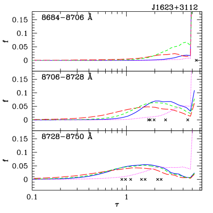
Figure 4.— Distributions of simulated optical depths for the three wavelength bins used in our analysis of J1623+3112. The solid blue, long-dashed red, short-dashed green, and dotted purple curves correspond to parameter combinations of ($R_{S}$, $x_{\rm HI}^{\rm IGM}$, $f_{\Gamma}$) = (29 Mpc, 1.0, 0.7), (29 Mpc, 0.04, 0.7), (33 Mpc, 1.0, 0.7), and (29 Mpc, 1.0, 0.1), respectively. The crosses are located at the set of observed optical depth values. The solid blue curve corresponds to the parameter combination with the peak likelihood value, while the parameter combinations represented by the other curves have likelihood values below 1/27th of the peak. The sharp jump at the largest $\tau$ bin and the overlaying of seven crosses in the top panel are due to the finite detection threshold, whereby all values of $\tau>5.5$ are indistinguishable from one another, and hence fall in the same bin in this figure. The figure demonstrates that our lower limit on $x_{\rm HI}^{\rm IGM}$ comes from the low–$\tau$ tail predicted in models with low neutral fractions or those corresponding to regions of parameter space which could mimic a low neutral fraction (see the discussion on isocontours in § 3). No points corresponding to these tails are seen in the data. Note also that while some models might perform well in one wavelength bin, only the solid blue curve is consistent with the observed data in all wavelength bins.

4. Discussion

In this section, we discuss a few important aspects of the above results. First, it is encouraging that the simple methodology we outlined can deliver statistically interesting constraints, even from the few dozen available spectral pixels. Clearly, it will be interesting to apply a similar analysis to a larger sample of sources in the future.

Perhaps our most interesting result is the lower limit we obtain, for two of the quasars, on the neutral fraction. We would like to therefore understand where these constraints actually come from. To this end, in Figure 4 we show the simulated optical depth PDFs for the three wavelength bins used in our analysis of J1623+3112. The solid blue, long-dashed red, short-dashed green, and dotted purple curves correspond to parameter combinations of ($R_{S}$, $x_{\rm HI}^{\rm IGM}$, $f_{\Gamma}$) = (29 Mpc, 1.0, 0.7), (29 Mpc, 0.04, 0.7), (33 Mpc, 1.0, 0.7), and (29 Mpc, 1.0, 0.1), respectively. The crosses are located at the set of observed optical depth values. The solid blue curve corresponds to the parameter combination with the peak likelihood value, while the parameter combinations represented by the other curves have likelihood values below 1/27th of the peak. The sharp jump corresponding at the largest $\tau$ bin and the overlaying of seven crosses in the top panel are due to the finite detection threshold, whereby all values of $\tau>5.5$ are indistinguishable from one another, and hence fall in the same bin in this figure. The figure clearly demonstrates that our lower limit on $x_{\rm HI}^{\rm IGM}$ arises from the low–$\tau$ tail predicted in models with low neutral fractions or those corresponding to regions of parameter space which could mimic a low neutral fraction (see the discussion on isocontours in § 3). While the solid blue curves are consistent with the distribution of points, these other curves all have tails that are “too long”: no points corresponding to these tails are seen in the data. Note also that while some models might perform well in one wavelength bin, only the solid blue curve is consistent with the observed data in all wavelength bins.

4.1. Sanity Checks

As our analysis technique is as yet untested, it is useful to take a step back, and verify that our results make sense. As already mentioned, the likelihood iso–contours behave as expected. Here we discuss several other encouraging checks on the validity of our analysis. We caution the reader, however, that these are not meant to be a proof of the accuracy of our analysis, and instead should be regarded merely as consistency checks.

First, the procedure here recovers fairly well the result of our previous analysis in the case of J1030+0524 (Mesinger & Haiman, 2004). This need not be the case, since the nature of the two analysis procedures are different; namely, our previous work focused only on gross, approximate Ly$\alpha$ and Ly$\beta$ transmission features near the edge of the HII region. Nevertheless, in both cases, the peak likelihood occurs at the same value of $x_{\rm HI}^{\rm IGM}$ and $R_{S}$, with only the value of $f_{\Gamma}$ being somewhat larger here ($f_{\Gamma}$=1.0 instead of $f_{\Gamma}$=0.4 in Mesinger & Haiman 2004). We attribute this shift in $f_{\Gamma}$ primarily to the inclusion of wavelength bins further inward from the HII region edge, where the effects of $R_{S}$ and $x_{\rm HI}^{\rm IGM}$ are felt less strongly and $f_{\Gamma}$ wields the most statistical weight. In particular, the likelihoods in the two blue-most wavelength bins are comparable for $f_{\Gamma}=1.0$ and $f_{\Gamma}=0.4$ (given $x_{\rm HI}^{\rm IGM}=1.0$ and $R_{S}=41$Mpc); however, the likelihoods in the two red-most wavelength bins are $\sim$ 7–8 times greater for $f_{\Gamma}=1.0$ than $f_{\Gamma}=0.4$.

Second, our results on the neutral fraction agree in relative terms with estimates obtained from transmission in GP troughs (Fan et al., 2006a). J1030+0524 and J1623+3112 both have very dark GP troughs in Ly$\alpha$ and Ly$\beta$, and thus are only able to provide lower limits on the optical depth and corresponding neutral fraction; however, J1148+5251 has transmission gaps in the GP troughs, thus favoring a smaller optical depth and corresponding neutral fraction. This is qualitatively similar to our results: we were unable to constrain $x_{\rm HI}^{\rm IGM}$ from the spectra of J1148+5251  obtaining only a shallow peak in the likelihood at $x_{\rm HI}^{\rm IGM}=0.2$; however, both J1030+0524 and J1623+3112 had peak likelihoods at $x_{\rm HI}^{\rm IGM}=1$, and strongly prefer $x_{\rm HI}^{\rm IGM}\mathrel{\hbox to0.0pt{\lower 4.0pt\hbox{\hskip 1.0pt$\sim$}\hss}\raise 1.0pt\hbox{$>$}}0.04$.

Third, the maximum likelihoods of $f_{\Gamma}$ (i.e. the relative strength of the quasars’ ionizing luminosity) match the relative strengths of the quasars’ continua redward of Ly$\alpha$. The values of $f_{\Gamma}$ corresponding to the peak likelihoods are 1.6, 1.0, and 0.7 for J1148+5251  J1030+0524  and J1623+3112  respectively. Looking at Figure 2, one can note that this is also the order of the relative strengths of the quasars’ continua redward of Ly$\alpha$, as one would expect if the UV power-law indices and amount of obscuration didn’t vary greatly among the quasars.

Finally, the quasar with the smallest HII region, J1623+3112  with a peak likelihood at $R_{S}=29$ Mpc, also has the highest favored value of $x_{\rm HI}^{\rm IGM}=1.0$ and the lowest favored value of $f_{\Gamma}$. This makes sense, since a fainter quasar, embedded in a more neutral medium should have a smaller HII region, given a similar lifetime.

4.2. Uncertainties in the Intrinsic Emission Spectra

Although we have added gaussian noise to our inferred template spectrum, as described above, we wish to get a sense of how correlated errors, modifying the broader shape of the template spectrum, would affect our results. The general concern is that mis–estimates of the flux, correlated over many pixels, could potentially mimic the effect of shifts in our parameter space. To get a sense of the magnitude of this effect, we chose to vary the width of the fitted Ly$\alpha$ gaussian for quasar J1623+3112 and see how this modifies our results. Naively, one would expect a narrower Ly$\alpha$ emission line and an accompanying decrease in effective $\tau_{\rm obs}$ to cause a shift in the parameter space to regions favoring smaller optical depths (larger $R_{S}$, smaller $x_{\rm HI}^{\rm IGM}$, larger $f_{\Gamma}$), with the opposite trends for a wider Ly$\alpha$ emission line.

We find that such degeneracies are very weak. For a 10% narrower line, we find that the peak likelihood remains at the same parameter–combinations. The range of parameter values whose likelihood estimates are within a factor of 3 of the peak likelihood changes by at most one pixel in our 3D parameter grid: 25 Mpc $\mathrel{\hbox to0.0pt{\lower 4.0pt\hbox{\hskip 1.0pt$\sim$}\hss}\raise 1.0pt\hbox{$<$}}R_{S}\mathrel{\hbox to0.0pt{\lower 4.0pt\hbox{\hskip 1.0pt$\sim$}\hss}\raise 1.0pt\hbox{$<$}}$ 29 Mpc; 0.008 $\mathrel{\hbox to0.0pt{\lower 4.0pt\hbox{\hskip 1.0pt$\sim$}\hss}\raise 1.0pt\hbox{$<$}}x_{\rm HI}^{\rm IGM}\mathrel{\hbox to0.0pt{\lower 4.0pt\hbox{\hskip 1.0pt$\sim$}\hss}\raise 1.0pt\hbox{$<$}}$ 1.0; 0.4 $\mathrel{\hbox to0.0pt{\lower 4.0pt\hbox{\hskip 1.0pt$\sim$}\hss}\raise 1.0pt\hbox{$<$}}f_{\Gamma}\mathrel{\hbox to0.0pt{\lower 4.0pt\hbox{\hskip 1.0pt$\sim$}\hss}\raise 1.0pt\hbox{$<$}}$ 1.6. This is a rather small change, and we emphasize that a 10% narrower Ly$\alpha$ line would actually be an unacceptably poor fit to the (red side of the) observed spectrum. A wider Ly$\alpha$ line is more physically motivated, since strong damping wing absorption might be able to somewhat attenuate flux far into the red side of the line. Hence, we vary the width of the Ly$\alpha$ line, well in excess of the absorbing potential of a strong damping wing. Again, we find little change in our results. Even for a 50% wider line, the parameter combination at peak likelihood remains the same, while the range of parameter values whose likelihood estimates are within a factor of 3 of the peak likelihood changes by at most one pixel to: 25 Mpc $\mathrel{\hbox to0.0pt{\lower 4.0pt\hbox{\hskip 1.0pt$\sim$}\hss}\raise 1.0pt\hbox{$<$}}R_{S}\mathrel{\hbox to0.0pt{\lower 4.0pt\hbox{\hskip 1.0pt$\sim$}\hss}\raise 1.0pt\hbox{$<$}}$ 31 Mpc; 0.2 $\mathrel{\hbox to0.0pt{\lower 4.0pt\hbox{\hskip 1.0pt$\sim$}\hss}\raise 1.0pt\hbox{$<$}}x_{\rm HI}^{\rm IGM}\mathrel{\hbox to0.0pt{\lower 4.0pt\hbox{\hskip 1.0pt$\sim$}\hss}\raise 1.0pt\hbox{$<$}}$ 1.0; 0.4 $\mathrel{\hbox to0.0pt{\lower 4.0pt\hbox{\hskip 1.0pt$\sim$}\hss}\raise 1.0pt\hbox{$<$}}f_{\Gamma}\mathrel{\hbox to0.0pt{\lower 4.0pt\hbox{\hskip 1.0pt$\sim$}\hss}\raise 1.0pt\hbox{$<$}}$ 1.3. As expected, an intrinsically wider Ly$\alpha$ line shows a slight preference for a more neutral universe.

Overall, the above exercise suggests that our results are robust and conservative, at least to mis–estimates of the Ly$\alpha$ line width. This does not, of course, preclude the possibility that the intrinsic Ly$\alpha$ lines of the $z\approx 6$ quasars possess some deviations from a gaussian shape. For example, if there is an asymmetry, in the sense of a steeper drop of flux on the blue side of the line than on the red side, our technique would have mistakenly attributed this steeper drop to absorption. This implies that we might have overestimated the neutral fractions. At present, there is, however, no evidence of such an asymmetry in the emission lines of low redshift quasars (where both sides of the lines can be seen unabsorbed), nor is there evidence, from the red side of the lines, that the high–$z$ quasars’ lines have shapes different from those of their lower–redshift counterparts.

Finally, we also note that our spectral fits, describing the intrinsic emission line on the unabsorbed red side of the line, leave typical flux residuals of only $\sim 1\%$. Similar residuals are presumably present on the blue side of the line, as well. However, the absorption $\exp(-\tau_{D})$ caused by the IGM damping wing on the blue side of the line (see Fig. 1), has an amplitude of $\sim(0.1--1)x_{\rm HI}$, exceeding the residuals for $x_{\rm HI}\mathrel{\hbox to0.0pt{\lower 4.0pt\hbox{\hskip 1.0pt$\sim$}\hss}\raise 1.0pt\hbox{$>$}}0.01$. Furthermore, in order for the residuals to mimic the IGM damping wing, they would have to be coherent (monotonically increasing with wavelength).

4.3. Biases in Local Density and Velocity Fields

As mentioned above, we remove the region 20–30 Å blueward of the line center from our analysis, corresponding to the expected mean radius of the large–scale overdense region surrounding such quasars (Barkana & Loeb, 2004a). This is a necessary step as present-day simulations cannot statistically model such rare, large–scale overdensities. However, if the density bias extended into our region of analysis, our inferred $x_{\rm HI}^{\rm IGM}$ lower limits would be conservative and our inferred $f_{\Gamma}$ values would most likely be underestimated. If the source is hosted by a large–scale overdensity, then density would decrease with decreasing $\lambda_{\rm obs}$ (increasing distance from the source). If such a decreasing density extended into our region of analysis, it would translate into a shallower rise in $\tau_{R}\propto n^{2}/\Gamma$. In matching the total optical depth $\tau_{\rm Ly\alpha}=\tau_{R}+\tau_{D}$, our analysis, which assumes constant mean density, would translate this shallower rise in $\tau_{R}$ to a shallower rise in $\tau_{D}$, i.e. a lower value of $x_{\rm HI}^{\rm IGM}$ than appropriate if the density bias was taken into account. Note that our results on $x_{\rm HI}^{\rm IGM}$ are driven by the wavelength dependence of $\tau$; a constant offset in the density field can be absorbed by a shift in $\Gamma_{\rm Q}$ (i.e. $f_{\Gamma}$), which dominates over $\Gamma_{\rm BG}$ throughout most of our region of interest and is predominantly set by the amount of absorption in bins further from the HII region edge where it has the most statistical weight. Furthermore, it is possible that an infalling IGM could introduce a similar bias, but the effect is likely to be small for a bright quasar and far away from the line center on the blue side. Moreover, the effect from the infall would have the same sign as the density bias above, making the flux fall off on the blue side of the line less steeply (Dijkstra et al., 2006; Barkana & Loeb, 2003)). In other words, by ignoring the possible density and velocity biases, we might only be slightly underestimating the neutral fraction.

4.4. Uncertainties in Intrinsic Redshift

A different source of possible error, in estimates of $R_{S}$, can result from an incorrect redshift determination. The redshifts we quote above were determined from high-ionization lines such as C IV, Si IV and N V. However, high-ionization emission lines can have non-negligible offsets from low-ionization, narrow, or molecular lines in the host galaxy. Recently, redshift determinations based on such lines have been made for the three quasars used in our analysis: $z_{\rm CO}=6.42$ for J1148+5251 (Walter et al., 2003); $z_{\rm MgII}=6.31$ for J1030+0524 (Iwamuro et al., 2004); $z_{\rm MgII}=6.22$ for J1623+3112 (L. Jiang et al. 2006, in preparation). These redshift determinations agree with the ones based on high-ionization lines used in this work for J1148+5251 and J1623+3112; however the Mg II redshift is 0.03 larger than the high-ionization line redshift for J1030+0524. If one takes the Mg II redshift to be the true systematic redshift, this would roughly increase all $R_{S}$ determinations for J1030+0524 by $\sim$ 30% The majority of the effect would be confined to the increase in $R_{S}$, since the systematic redshift doesn’t impact the Ly$\alpha$ emission fitting, and the isocontours (as seen in the middle panels of Fig. 3) are steep (i.e. a large increase in $R_{S}$ can be compensated for by a small increase in $x_{\rm HI}^{\rm IGM}$, especially for the lower confidence contours). Since increasing $R_{S}$ can roughly be compensated for by increasing $x_{\rm HI}^{\rm IGM}$ or decreasing $f_{\Gamma}$, the secondary effects of such a redshift underestimate should be a shift in the favored parameter values towards larger $x_{\rm HI}^{\rm IGM}$ and/or smaller $f_{\Gamma}$.

5. Conclusions

We have made use of hydrodynamical simulations of the IGM to create model quasar absorption spectra, and compared these with observed Keck ESI spectra of three $z>6.2$ quasars: J1148+5251 ($z=6.42$), J1030+0524 (z=6.28), and J1623+3112 (z=6.22). We compared the CPDFs of observed Ly$\alpha$ optical depths to those generated from the simulation by assuming various values for the size of the quasar’s surrounding HII region, $R_{S}$ (in comoving Mpc), volume-weighted neutral hydrogen fraction in the ambient IGM, $\bar{x}_{\rm HI}$, and the quasar’s emission rate of ionizing photons, $\dot{N}_{Q}$ (in 10⁵⁷ s^-1). This approach has not yet been applied to the spectra of the $z\mathrel{\hbox to0.0pt{\lower 4.0pt\hbox{\hskip 1.0pt$\sim$}\hss}\raise 1.0pt\hbox{$>$}}6$ quasars, and we have emphasized some important caveats, most importantly our neglect of radiative transfer effects, and our assumption that the intrinsic emission line of the quasars is symmetric around the line center. Since large sightline-to-sightline fluctuations in IGM properties are likely at these high-redshifts, we analyzed each quasar independently. We found that our approach can constrain $R_{S}$ to within $\sim$ 10%, and $\dot{N}_{Q}$ to within a factor of $\sim$ 2 for all three quasars. Fairly strong constraints on $\bar{x}_{\rm HI}$ are obtained from J1030+0524 and J1623+3112, while $\bar{x}_{\rm HI}$ is unconstrained by J1148+5251. Specifically, our results are as follows.

J1148+5251: the parameter combination with the maximum likelihood is ($R_{S}$, $\bar{x}_{\rm HI}$, $\dot{N}_{Q}$) = (40, 0.16, 2.1); the range of parameter values whose likelihood estimates are within a factor of three of the peak is encompassed by: $40\mathrel{\hbox to0.0pt{\lower 4.0pt\hbox{\hskip 1.0pt$\sim$}\hss}\raise 1.0pt\hbox{$<$}}R_{S}\mathrel{\hbox to0.0pt{\lower 4.0pt\hbox{\hskip 1.0pt$\sim$}\hss}\raise 1.0pt\hbox{$<$}}42$, $\bar{x}_{\rm HI}\mathrel{\hbox to0.0pt{\lower 4.0pt\hbox{\hskip 1.0pt$\sim$}\hss}\raise 1.0pt\hbox{$<$}}1$, $0.9\mathrel{\hbox to0.0pt{\lower 4.0pt\hbox{\hskip 1.0pt$\sim$}\hss}\raise 1.0pt\hbox{$<$}}\dot{N}_{Q}\mathrel{\hbox to0.0pt{\lower 4.0pt\hbox{\hskip 1.0pt$\sim$}\hss}\raise 1.0pt\hbox{$<$}}2.5$.

J1030+0524: the parameter combination with the maximum likelihood is ($R_{S}$, $\bar{x}_{\rm HI}$, $\dot{N}_{Q}$) = (41, 1, 1.3); the range of parameter values within a factor of three of the peak likelihood is encompassed by: $41\mathrel{\hbox to0.0pt{\lower 4.0pt\hbox{\hskip 1.0pt$\sim$}\hss}\raise 1.0pt\hbox{$<$}}R_{S}\mathrel{\hbox to0.0pt{\lower 4.0pt\hbox{\hskip 1.0pt$\sim$}\hss}\raise 1.0pt\hbox{$<$}}45$, $0.033\mathrel{\hbox to0.0pt{\lower 4.0pt\hbox{\hskip 1.0pt$\sim$}\hss}\raise 1.0pt\hbox{$<$}}\bar{x}_{\rm HI}$, $0.9\mathrel{\hbox to0.0pt{\lower 4.0pt\hbox{\hskip 1.0pt$\sim$}\hss}\raise 1.0pt\hbox{$<$}}\dot{N}_{Q}\mathrel{\hbox to0.0pt{\lower 4.0pt\hbox{\hskip 1.0pt$\sim$}\hss}\raise 1.0pt\hbox{$<$}}1.7$.

J1623+3112: the parameter combination with the maximum likelihood is ($R_{S}$, $\bar{x}_{\rm HI}$, $\dot{N}_{Q}$) = (29, 1, 0.9); the range of parameter values within a factor of three of the peak likelihood is encompassed by: $25\mathrel{\hbox to0.0pt{\lower 4.0pt\hbox{\hskip 1.0pt$\sim$}\hss}\raise 1.0pt\hbox{$<$}}R_{S}\mathrel{\hbox to0.0pt{\lower 4.0pt\hbox{\hskip 1.0pt$\sim$}\hss}\raise 1.0pt\hbox{$<$}}29$, $0.033\mathrel{\hbox to0.0pt{\lower 4.0pt\hbox{\hskip 1.0pt$\sim$}\hss}\raise 1.0pt\hbox{$<$}}\bar{x}_{\rm HI}$, $0.5\mathrel{\hbox to0.0pt{\lower 4.0pt\hbox{\hskip 1.0pt$\sim$}\hss}\raise 1.0pt\hbox{$<$}}\dot{N}_{Q}\mathrel{\hbox to0.0pt{\lower 4.0pt\hbox{\hskip 1.0pt$\sim$}\hss}\raise 1.0pt\hbox{$<$}}1.7$.

It is encouraging that the simple methodology we have utilized can deliver statistically interesting constraints, even from the few dozen available spectral pixels. Our method is different from previous analyses of the GP absorption spectra of these quasars, and the lower limits we found on the neutral fraction of the IGM surrounding two of the quasars strengthen the evidence that the rapid end–stage of reionization is occurring near $z\sim 6$. Clearly, it will be interesting to apply a similar analysis to a larger sample of sources in the future.

References

- Bajtlik et al. (1988) Bajtlik, S., Duncan, R. C., & Ostriker, J. P. 1988, ApJ, 327, 570
- Barkana & Loeb (2003) Barkana, R., & Loeb, A. 2003, Nature, 421, 341
- Barkana & Loeb (2004a) —. 2004a, ApJ, 601, 64
- Barkana & Loeb (2004b) —. 2004b, ApJ, 609, 474
- Bolton & Haehnelt (2006) Bolton, J. S., & Haehnelt, M. G. 2006, ArXiv Astrophysics e-prints
- Cen (1994) Cen, R. 1994, ApJ, 437, 12
- Cen et al. (2005) Cen, R., Haiman, Z., & Mesinger, A. 2005, ApJ, 621, 89
- Cen et al. (2003) Cen, R., Ostriker, J. P., Prochaska, J. X., & Wolfe, A. M. 2003, ApJ, 598, 741
- Dijkstra et al. (2006) Dijkstra, M., Haiman, Z., & Spaans, M. 2006, ApJ, 649, 37
- Djorgovski et al. (2006) Djorgovski, S. G., Bogosavljevic, M., & Mahabal, A. 2006, New Astronomy Review, 50, 140
- Elvis et al. (1994) Elvis, M. et al. 1994, ApJS, 95, 1
- Fan et al. (2002) Fan, X., Narayanan, V. K., Strauss, M. A., White, R. L., Becker, R. H., Pentericci, L., & Rix, H. 2002, AJ, 123, 1247
- Fan et al. (2006a) Fan, X. et al. 2006a, AJ, 132, 117
- Fan et al. (2006b) —. 2006b, AJ, 131, 1203
- Furlanetto et al. (2004a) Furlanetto, S. R., Hernquist, L., & Zaldarriaga, M. 2004a, MNRAS, 354, 695
- Furlanetto et al. (2004b) Furlanetto, S. R., Zaldarriaga, M., & Hernquist, L. 2004b, ApJ, 613, 1
- Furlanetto et al. (2006) —. 2006, MNRAS, 365, 1012
- Gallerani et al. (2006) Gallerani, S., Choudhury, T. R., & Ferrara, A. 2006, MNRAS, 370, 1401
- Greene & Ho (2004) Greene, J. E., & Ho, L. C. 2004, ApJ, 610, 722
- Haiman & Cen (2002) Haiman, Z., & Cen, R. 2002, ApJ, 578, 702
- Haiman & Cen (2005) —. 2005, ApJ, 623, 627
- Ho et al. (1997) Ho, L. C., Filippenko, A. V., Sargent, W. L. W., & Peng, C. Y. 1997, ApJS, 112, 391
- Iwamuro et al. (2004) Iwamuro, F., Kimura, M., Eto, S., Maihara, T., Motohara, K., Yoshii, Y., & Doi, M. 2004, ApJ, 614, 69
- Kashikawa et al. (2006) Kashikawa, N. et al. 2006, ApJ, 648, 7
- Kohler et al. (2005) Kohler, K., Gnedin, N. Y., & Hamilton, A. J. S. 2005, ArXiv Astrophysics e-prints
- Lewis (2006) Lewis, A. 2006, ArXiv Astrophysics e-prints
- Lidz et al. (2006) Lidz, A., Oh, S. P., & Furlanetto, S. R. 2006, ApJ, 639, L47
- Malhotra & Rhoads (2004) Malhotra, S., & Rhoads, J. E. 2004, ApJ, 617, L5
- Maselli et al. (2006) Maselli, A., Gallerani, S., Ferrara, A., & Choudhury, T. R. 2006, ArXiv Astrophysics e-prints
- Mesinger & Haiman (2004) Mesinger, A., & Haiman, Z. 2004, ApJ, 611, L69
- Mesinger et al. (2004) Mesinger, A., Haiman, Z., & Cen, R. 2004, ApJ, 613, 23
- Oh & Furlanetto (2005) Oh, S. P., & Furlanetto, S. R. 2005, ApJ, 620, L9
- Page et al. (2006) Page, L. et al. 2006, ApJ, submitted
- Peebles (1993) Peebles, P. J. E. 1993, Principles of physical cosmology (Princeton Series in Physics, Princeton, NJ: Princeton University Press, —c1993)
- Press et al. (1992) Press, W. H., Teukolsky, S. A., Vetterling, W. T., & Flannery, B. P. 1992, Numerical recipes in C. The art of scientific computing (Cambridge: University Press, —c1992, 2nd ed.)
- Rollinde et al. (2005) Rollinde, E., Srianand, R., Theuns, T., Petitjean, P., & Chand, H. 2005, MNRAS, 361, 1015
- Spergel et al. (2006a) Spergel, D. N. et al. 2006a, ApJ, submitted, preprint astro-ph/0603449
- Spergel et al. (2006b) —. 2006b, ApJ, submitted
- Telfer et al. (2002) Telfer, R. C., Zheng, W., Kriss, G. A., & Davidsen, A. F. 2002, ApJ, 565, 773
- Totani et al. (2006) Totani, T., Kawai, N., Kosugi, G., Aoki, K., Yamada, T., Iye, M., Ohta, K., & Hattori, T. 2006, PASJ, 58, 485
- Vanden Berk et al. (2001) Vanden Berk, D. E. et al. 2001, AJ, 122, 549
- Walter et al. (2003) Walter, F. et al. 2003, Nature, 424, 406
- White et al. (2003) White, R. L., Becker, R. H., Fan, X., & Strauss, M. A. 2003, AJ, 126, 1
- Wyithe & Loeb (2004) Wyithe, J. S. B., & Loeb, A. 2004, Nature, 427, 815
- Wyithe & Loeb (2006) Wyithe, S., & Loeb, A. 2006, ArXiv Astrophysics e-prints