Supernovae in Low-Redshift Galaxy Clusters:
the Type-Ia Supernova Rate

Abstract

Supernova (SN) rates are a potentially powerful diagnostic of star formation history (SFH), metal enrichment, and SN physics, particularly in galaxy clusters with their deep, metal-retaining potentials, and simple SFH. However, a low-redshift cluster SN rate has never been published. We derive the SN rate in galaxy clusters at $0.06<z<0.19$, based on type Ia supernovae (SNe Ia) that were discovered by the Wise Observatory Optical Transient Survey. As described in a separate paper, a sample of 140 rich Abell clusters was monitored, in which six cluster SNe Ia were found and confirmed spectroscopically. Here, we determine the SN detection efficiencies of the individual survey images, and combine the efficiencies with the known spectral properties of SNe Ia to calculate the effective visibility time of the survey. The cluster stellar luminosities are measured from the Sloan Digital Sky Survey (SDSS) database in the $griz$ SDSS bands. Uncertainties are estimated using Monte-Carlo simulations in which all input parameters are allowed to vary over their known distributions. We derive SN rates normalized by stellar luminosity, in SNU units (SNe per century per $10^{10}L_{\odot}$) in five photometric bandpasses, of $0.36^{+0.22}_{-0.14}\pm 0.02$ ($B$), $0.351^{+0.210}_{-0.139}\pm 0.020$ ($g$), $0.288^{+0.172}_{-0.114}\pm 0.018$ ($r$), $0.229^{+0.137}_{-0.091}\pm 0.014$ ($i$), $0.186^{+0.111}_{-0.074}\pm 0.010$ ($z$), where the quoted errors are statistical and systematic, respectively. The SN rate per stellar mass unit, derived using a color-luminosity-mass relation, is $0.098^{+0.059}_{-0.039}\pm 0.009$  SNe (century $10^{10}M_{\sun}$)^-1. The low cluster SN rates we find are similar to, and consistent with, the SN Ia rate in local elliptical galaxies.

1. Introduction

The event-rate history of supernovae (SNe), their progenitor systems, and the physical mechanisms behind these explosions, all have important implications for several branches of astrophysics and cosmology. As the primary sources of iron and other heavy elements, SNe have a key role in the chemical evolution of the Universe (e.g., Nomoto et al. 2005). The history of enrichment is determined by the rate of SNe in the past and by the inventory of heavy elements that is released by each explosion. In cosmology, type Ia SNe (SNe Ia) used as cosmological distance indicators have provided direct evidence for an accelerated expansion of the Universe (e.g., Riess et al. 1998, 2004; Perlmutter et al. 1999; Astier et al. 2006). The use of SNe Ia as standard candles relies on the assumptions that there is no evolution in their intrinsic properties, and that their luminosities can be calibrated through an unevolving empirical relation to their light-curve shape (for reviews, see Leibundgut 2001; Filippenko 2004, 2005). If these assumptions could be founded on more solid observational and physical grounds, the cosmological use of SNe Ia would stand on a firmer footing.

It is widely agreed that SNe Ia occur when a white dwarf in a binary system is pushed toward the Chandrasekhar mass limit and undergoes a runaway thermonuclear explosion. However, there is no consensus regarding how this situation is reached. In the single-degenerate scenario, a white dwarf accretes matter from a main-sequence, subgiant, or giant star. In the double-degenerate scenario, two white dwarfs merge. Furthermore, it is not clear how the explosion proceeds. Since direct observational identification of a SN Ia progenitor system is unlikely, indirect evidence may be the only practical way to distinguish between models. Modeling of the observed spectra of SNe provides many clues (e.g., Nomoto et al. 1984), as do studies of Galactic SN remnants (e.g., Badenes et al. 2006). However, these studies mostly constrain the explosion physics (deflagration or detonation) and are less sensitive to the identity of the mass donor.

A complementary approach exploits the fact that each of the above scenarios may predict a “time delay distribution,” which is the distribution of times elapsed between the formation of a stellar population and the explosions of some members of the population as SNe Ia (e.g., Yungelson & Livio 2002; Greggio 2005; Förster et al. 2006). The time delay, in turn, convolved with the star formation history (SFH), dictates the evolution of the SN rate with cosmic time or with redshift. By measuring the SN Ia rate vs. redshift $z$, one can, in principle, constrain the form of the time delay distribution and obtain clues about the progenitor scenario (e.g., Pain et al. 2002; Gal-Yam & Maoz 2004; Strolger et al. 2004; Sullivan et al. 2006; Barris & Tonry 2006; Neill et al. 2006; Förster et al. 2006).

In practice, there are several complications. A prediction of the SN rate is sensitive to the assumed SFH. For example, Förster et al. (2006) recently re-analyzed the SN Ia sample of Strolger et al. (2004) and argued that, by varying the choice of SFH within the uncertainties allowed by observations, a wide range of time delay distributions are consistent with the SN data, and hence none of the SN Ia scenarios can be ruled out. Another complication follows from the recent evidence that SNe Ia are descended from two distinct stellar populations (Mannucci et al. 2005; Scannapieco & Bildsten 2005; Sullivan et al. 2006), perhaps leading to two SN Ia “channels” – a “prompt” channel, with a delay time of order 1 Gyr or less, and a “delayed” channel, with delay times that extend to $\gtrsim 10$ Gyrs. Effectively, this means a time delay distribution that is more complex than those predicted by single-channel models. The combination of these two issues, combined with debates regarding sample completeness, have prevented conclusive determinations of delay times.

Measuring the SN Ia delay time in galaxy clusters, however, may provide a solution to these difficulties. Analysis of the stellar population of cluster galaxies suggests that the SFH in clusters is simpler than that in the field, and can likely be approximated by a brief starburst at high redshift (e.g., Wuyts et al. 2004; Holden et al. 2005). Sullivan et al. (2006) show that the mix between the delayed and prompt components of the SN Ia population changes in different environments. The prompt component dominates late-type galaxies, while elliptical galaxies contain only members of the delayed group. SN rate measurements in clusters could then provide an estimate of the delayed component alone with minimal contamination. If the population of SNe Ia is indeed bimodal, pinning down one of its components from cluster SN studies could help to disentangle the two populations in the field.

Furthermore, measurement of cluster SN rates may help resolve the question of the dominant source of the high metallicity in the intracluster medium (e.g., Renzini et al. 1993; Maoz & Gal-Yam 2004) – SNe Ia, or core-collapse SNe from an early stellar population with a top-heavy initial mass function (e.g., Maoz & Gal-Yam 2004; Loewenstein 2006). Clusters are excellent laboratories for studying enrichment, due to their simple SFH and their deep potentials from which matter cannot escape. Therefore, understanding the source of intracluster metals would be relevant for understanding metal enrichment in general, and the possible role of first-generation stars in early-universe enrichment.

Although SN Ia rates have been measured extensively out to $z\approx 1$ (Pain et al. 1996, 2002; Cappellaro et al. 1999; Hardin et al. 2000; Tonry et al. 2003; Madgwick et al. 2003; Blanc et al. 2004; Dahlén et al. 2004; Barris & Tonry 2006; Neill et al. 2006), there have been few attempts to measure the SN rate in galaxy clusters (e.g., Barbon 1978; Norgaard-Nielsen et al. 1989; Reiss et al. 1998). The only published cluster SN rate at distances beyond the Virgo cluster is by Gal-Yam, Maoz, & Sharon (2002). This measurement was based on the detection of two or three likely cluster SNe Ia in archival Hubble Space Telescope (HST) images of high-redshift clusters. The derived rates, $0.39^{+0.59}_{-0.25}$ SNu_B at $z=0.25$ and $0.80^{+0.92}_{-0.40}$ SNu_B at $z=0.9$ [$1$ SNu_B $=1$ SN century${}^{-1}(10^{10}L_{B,\sun})^{-1}]$, have large uncertainties due to the small number of detected SNe and the lack of follow-up observations, a consequence of searching archival data.

We are carrying out a program to measure the cluster SN rate at both low and high redshifts. In this paper, we derive the cluster SN rate based on a low-redshift ($0.06<z<0.19$) cluster SN survey, the Wise Observatory Optical Transient Search (WOOTS).

The cluster sample, the observational design, and the SN detection, spectroscopic follow-up observations, and classification are described in a separate paper by Gal-Yam et al. (2006), hereafter Paper I.

Here, we present the details of the derivation of the cluster SN rate and briefly discuss its implications.

Throughout the paper we assume a flat cosmology, with parameters $\Omega_{\Lambda}=0.7$, $\Omega_{\rm M}=0.3$, and $H_{0}=70~{}{\rm km~{}s}^{-1}{\rm Mpc}^{-1}$.

2. The Survey

In Paper I, we present the observational details of WOOTS, the SNe that were discovered by it, and their followup observations. Briefly, WOOTS was a survey for SNe and other transient or variable sources in the fields of 161 galaxy clusters, and was conducted in 1997-1999. The cluster sample was selected from the catalog of Abell, Corwin & Olowin (1984), based on the following criteria: cluster redshift in the range $0.06<z<0.2$ (based on the compilation of Struble & Rood 1991); declination $\delta>0$; Abell richness class $R\geq 1$ (Abell galaxy count $N>65$); and cluster radius (estimated by Leir & Van den Bergh 1977) smaller than $20^{\prime\prime}$. Monthly dark-time observations used the Wise Observatory 1 m telescope, with a $1024\times 1024$, $0\farcs 7$ pixel, Tektronics CCD imager, giving a $12^{\prime}\times 12^{\prime}$ field of view. Images were unfiltered (see also § 3) reaching a limiting magnitude equivalent to $R\sim 22$. Images (of $\sim 40$ clusters per night) were compared with previously obtained template images using image subtraction methods, and searched for transients.

All candidate transients were followed up photometrically at Wise, and spectroscopically with larger telescopes. The determination of SN redshifts, ages and types was done by comparing the observed spectra to redshifted versions of high S/N template spectra of nearby SNe, drawn from the spectroscopic archive presented by Poznanski et al. (2002). In the course of the survey, 12 SNe were discovered, all of them spectroscopically confirmed (11 as type-Ia, and one as a type-IIP SN). Seven of the SNe (all of them SNe Ia) were in their respective clusters, and the remaining five were foreground and background events. All additional transient/variable candidates were confirmed as non-SN events: asteroids, active galactic nuclei, and variable stars.

The SN sample we will analyze in this paper does not include SN 2001al (Gal Yam et al. 2003), a cluster SN Ia which was discovered during an extension of WOOTS using a new CCD camera during its commissioning phase. We do not consider in this paper any of the survey images from that survey extension. In addition, we do not include in our analysis a sub-sample of 21 clusters for which the imaging data were inadvertently lost. Our sample thus consists of six confirmed cluster SNe Ia that were discovered by monitoring, effectively, $140$ Abell clusters at $0.06<z<0.19$. Table 1 lists the six events and their main parameters.

Table 1WOOTS Cluster SNe Ia

SN	Cluster	Redshift
1998fc	Abell 403	0.10
1998eu	Abell 125	0.18
1999cg	Abell 1607	0.14
1999ch	Abell 2235	0.15
1999ci	Abell 1984	0.12
1999ct	Abell 1697	0.18

3. Photometric Calibration

A derivation of the SN rate from our survey requires knowledge of the depth of all the survey images, and hence a photometric calibration of the survey data in the observed bandpass. The WOOTS images were obtained in unfiltered (“clear”) mode, resulting in a very broad, nonstandard photometric bandpass. We have determined the effective WOOTS-clear bandpass by multiplying the quantum efficiency curve of the back-illuminated, Lumogen-coated, Tektronix CCD used in the survey, by the typical atmospheric transmission at Wise Observatory for the mean airmass (1.2) of the WOOTS observations. We have verified that the effects of varying airmass and of mirror reflectivity vs. wavelength have negligible effect of the shape of the bandpass, The peak transmission of the effective WOOTS-clear band is at $\sim 7000$ Å, with a full-width at half maximum (FWHM) of $\sim 4700$ Å.

To obtain the individual photometric zeropoints of all the WOOTS images, we begin by using those images that fall within the coverage of the Sloan Digital Sky Survey Data Release 4 (SDSS DR4; Adelman-McCarthy et al. 2006). We extract the SDSS photometry of objects identified in each image and find the best fit to the SDSS $ugriz$ magnitudes from among a set of template spectra of stars (with spectral types O to M; Silva et al. 1992) and galaxies (Kinney et al. 1996). We then use the WOOTS-clear bandpass to perform synthetic, Vega-based photometry on the best-fit spectrum for each object. Finally, we compare these synthetic magnitudes to the instrumental magnitudes of the same objects, defined as $m_{\rm inst}=-2.5\log({\rm counts})$. The WOOTS zeropoint is then defined as the median of the differences between the synthetic and the instrumental magnitudes of the calibration sources in the image. The root-mean-square (rms) scatter of these differences defines the statistical zeropoint error for each image. Every source in an image can then be calibrated to a Vega-based WOOTS-clear magnitude by adding to its instrumental magnitude the derived zeropoint of the image. We estimate the accuracy of the zeropoints measured this way by adding the systematic uncertainty in the SDSS zeropoints ($0.02$ mag) to the statistical zeropoint error determined for each image, as defined above (typically also $0.02$ mag), resulting in a total zeropoint error of $0.04$ mag.

In order to calibrate the images that are in areas not covered by the SDSS, we compare the instrumental magnitudes of objects in our images with their “$R1$” magnitudes in the USNO-$B$ catalog (Monet et al. 2003), to get an “$R1$”-based zeropoint. The USNO-$R1$ band has a similar effective wavelength to that of the WOOTS-clear band, but is much narrower. From $329$ images in regions covered by the SDSS, we measure a mean offset of $0.24$ mag between the Vega-based unfiltered WOOTS zeropoint and the $R1$ zeropoint, and use it to calibrate the rest of the images. The scatter around this offset, $0.3$ mag, reflects both image-to-image scatter in the calibration process (e.g., due to variations in the mix of spectral types among the lists of calibration objects), and systematic errors in the USNO-$B$ photometry. The photometric accuracy of USNO-$B$ is not well determined, but Monet et al. (2003) estimate that the scatter in the photometric solution over the entire catalog has an rms of $0.25$ mag, consistent with our results. We therefore adopt $0.3$ mag as the zeropoint error of the non-SDSS images. These calibration uncertainties affect the overall uncertainty in the SN rate, through the determination of our search efficiency and the visibility time (see § 5).

4. SN Rate Calculation

Given a sample of $N$ SNe discovered as part of a survey, the SN rate per unit stellar luminosity is

$${\cal R}_{\rm Ia}=\frac{N}{\sum\limits_{j}{\Delta t_{j}L_{band,j}}},$$ (1)

where $\Delta t_{j}$ is the effective visibility time (or “control time”), i.e., the time during which a cluster SN Ia is above the detection limit of the $j$th image, $L_{band,j}$ is the cluster luminosity within the search area in a chosen photometric band, and the summation is over all the survey images. We explain below our measurement of each of these variables in the present survey.

4.1. Visibility Time and Light Curves

The effective visibility time, $\Delta t_{j}$, can be understood as the amount of time during which the survey is sensitive to SNe in a comparison between two particular images of a given cluster. This quantity depends on the SN detection efficiency in each image, the SN light curve at each cluster redshift, and on the frequency of searches in the same field. We calculate the effective visibility time from

$$\Delta t_{j}=\int^{\infty}_{-\infty}{\eta^{*}[m_{eff}(t)]dt},$$ (2)

where $m_{eff}(t)$ is an “effective” SN Ia light curve in the survey bandpass at the given redshift, as explained in § 4.1.2 below, and $\eta^{*}[m_{eff}(t)]$ is the detection probability as a function of SN effective magnitude. We describe below each step in this calculation.

4.1.1 Detection Efficiency Estimation

The detection efficiency of an image as a function of magnitude is the probability of detecting a SN-like point source in that image. In order to estimate the detection efficiency for a given field, we carry out simulations, following the prescription in Gal-Yam et al. (2002). About $200$ fake SNe are added blindly to each field, with a range of magnitudes, and with a spatial distribution that follows the flux of galaxies in the field. The simulated data undergo the same search procedure as the real data by means of difference image analysis (see Paper I), and the number of fake SNe that are successfully detected in each magnitude bin is noted. The SN detection efficiency is usually close to 100% 1–2 mag above the detection limit of the image, and drops roughly linearly to zero over this range (Fig. 1). We parametrize the efficiency curve with the function

$$\eta(m;m_{0.5},s,s_{2})=\left\{\begin{array}[]{ll}\left(1+e^{\frac{m-m_{0.5}}{s}}\right)^{-1},&\mbox{$m\leq m_{0.5}$}\\ \left(1+e^{\frac{m-m_{0.5}}{s_{2}}}\right)^{-1},&\mbox{$m>m_{0.5}$},\\ \end{array}\right.$$ (3)

where $m$ is the Vega-based magnitude of a SN in the effective bandpass of the survey (see below), $m_{0.5}$ is the magnitude at which the efficiency drops to $0.5$, and $s$ and $s_{2}$ determine the range of $m$ over which $\eta$ changes from $1$ to $0.5$ and from $0.5$ to zero, respectively. The main contribution to a slow convergence to unity at magnitudes brighter than $m_{0.5}$ is the difficulty of detecting SNe which lie close to, or are superposed on, the nucleus of a bright galaxy. Such cases are automatically included in our simulations when distributing the fake SNe in the images. Figure 1 shows four examples of the results of efficiency simulations, and the best-fit efficiency curves.

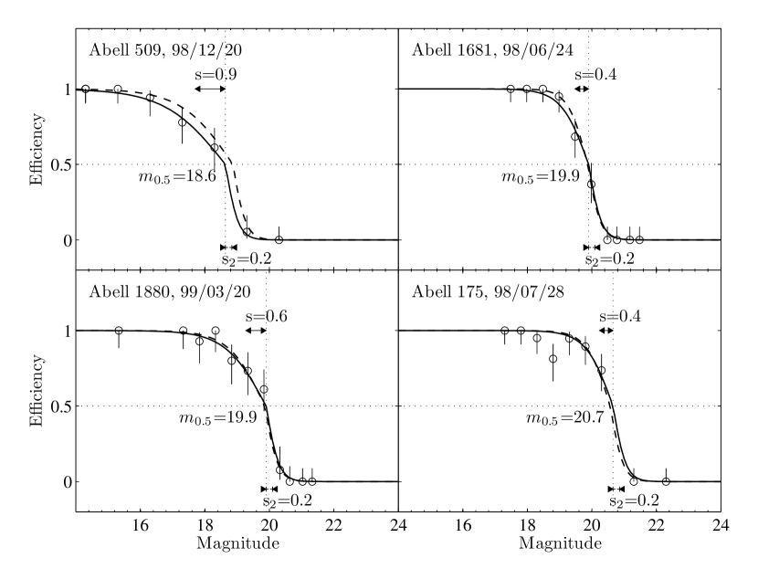
Figure 1.— Examples of point-source detection efficiency curves, as a function of WOOTS-clear Vega-based magnitude, for four survey images. Cluster names and observation dates are as marked. Circles mark the fraction of detected fake SNe, with error bars based on a binomial distribution. Solid curves are the best-fit efficiency curves (Eq. 3), and the dashed curves are the efficiency curves that correspond to the observational parameters of each image and the relations in Fig. 2.

The WOOTS database consists of $913$ images, which were obtained under a range of observing conditions – atmospheric transparency, mirror reflectivity, sky background, and telescope image quality. As a result, the detection efficiency varies significantly among the images. Since performing efficiency simulations in each and every image would be impractical, we have carried out simulations, as described above, for a subset of 30 images spanning a range in observing conditions. We then searched for correlations between the parameters of the resulting efficiency curves and various parameters that characterize each image. As detailed below, we found that the detection efficiency is primarily determined by two image parameters: the photometric zeropoint, which determines $m_{0.5}$, and the number of residuals that are left in each difference image, with which the upper slope parameter, $s$, is correlated. The lower slope parameter, $s_{2}$, did not vary significantly among the 30 simulated images, and was therefore set to its mean value, $0.2$.

The sensitivity of each image to SNe is determined by its photometric zeropoint, which combines the effects of detector quantum efficiency, variable mirror reflectivity, and variable atmospheric transparency. Specifically, the zeropoint, $ZP$, is an indicator of the limiting magnitude of the image, and therefore dictates the magnitude around which our detection efficiency drops rapidly. Figure 2 shows the relation that we have found between $ZP$ and $m_{0.5}$, $m_{0.5}=ZP-8.25$, with a scatter of $0.42$ mag.

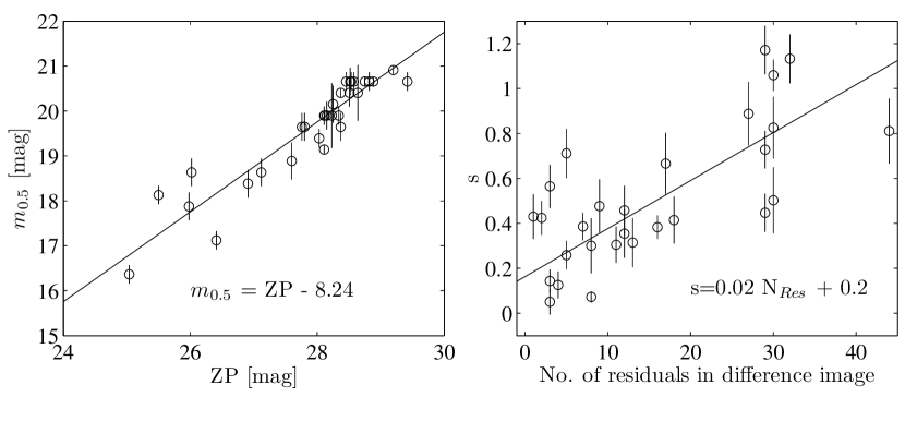
Figure 2.— Correlations between efficiency function parameters and image properties. Left: Magnitude at half the maximum efficiency ($m_{0.5}$) vs. image zeropoint ($ZP$), both in WOOTS-clear Vega magnitudes. Right: Exponential decline rate ($s$) vs. number of residuals in the difference image ($N_{Res}$).

The number of residuals, $N_{Res}$, was defined as the number of objects detected by SExtractor (Bertin & Arnouts 1996) in each difference image, with a detection threshold of $5\sigma$ above the background. A large number of subtraction residuals in an image can be due to several reasons. Most often, poor subtraction occurs when the point-spread function (PSF) in the image is very different from the PSF in the reference image. This happens when the PSF is distorted, e.g., due to imperfect telescope tracking, or atmospheric refraction at high airmass. Imperfect PSF matching and poor image subtraction will mostly affect the cores of bright galaxies, decreasing the chances of detecting SNe that lie close to galactic nuclei, and causing the efficiency curve to converge more slowly to the maximal detection efficiency. This behavior is parametrized by $s$. We find that $s$ depends on the number of residuals through the relation $s=0.02N_{Res}+0.3$, with an rms of $0.3$ (see Fig. 2).

We found no significant dependence of detection efficiency on the remaining observational parameters (sky background level and seeing width) due to the fact that most of the images were obtained during dark time, and the seeing spanned a limited range of $3\pm 0.4^{\prime\prime}$ FWHM. Based on the above relations, we can obtain efficiency curves for all images in the survey based on their measured observational parameters, $ZP$ and $N_{Res}$.

4.1.2 Light Curves

The peak magnitudes of SNe Ia exhibit an intrinsic rms scatter of 0.2–0.3 mag, and are correlated with the shape of the light curve through a stretch relation (Phillips 1993; see Leibundgut 2001 for a review). Since more luminous SNe tend to rise and decline more slowly than less luminous SNe, their overall visibility time is longer than that of dim SNe. Sullivan et al. (2006b) study the dependence of SN Ia properties on host-galaxy type, and show that SNe Ia in elliptical galaxies tend to be dimmer (with a smaller stretch factor). In their Fig. 11, they present the distribution of stretch factors according to galaxy type, at low and high redshifts. The bulk of the stellar light and mass in clusters is contributed by early-type galaxies. Indeed, among the six cluster SNe in our sample, the five with hosts were in early-type galaxies (one of the SNe was a hostless intergalactic cluster SN – see Gal-Yam et al. 2003). Assuming that all the SNe Ia in the clusters in our sample occur in elliptical galaxies, we use the distribution of stretch factors of SNe with elliptical hosts to assemble a dataset of light curves that will serve as templates. We base these light curves on a rest-frame, non-stretched, $B$-band template light curve from Nugent et al. (2002), and transform it to different stretched light curves using the stretch relation, $M_{s}=M_{s=1}-\alpha(s-1)$,$t_{s}=t_{s=1}\times\alpha$ as described by Perlmutter et al. (1999). For consistency, we use the same non-stretched peak $B$-band magnitude and $\alpha$ as Sullivan et al. (2006a), $M_{B}=-19.25$ (for h=0.7) and $\alpha=1.47$, which are based on the results of Knop et al. (2003). We assume an uncertainty of $0.15$ mag in $M_{B}$, from the dispersion in peak magnitudes of local SN light curves after stretch correction (Guy et al. 2005). This uncertainty is taken into account in our error budget (see § 5).

Since WOOTS observations were unfiltered, a transformation from the rest-frame $B$-band light curve to an observed WOOTS-clear light curve at the cluster redshift is necessary. For each cluster, we calculate a set of stretched SN light curves from multi-epoch SN Ia spectra, using synthetic photometry, as follows. We start with a set of multi-epoch spectral templates from Nugent et al. (2002). For each combination of stretch and redshift, we normalize the spectra to fit the $B$-band rest-frame photometry, and redshift them according to the cluster redshift. We then multiply the spectra by the WOOTS-clear bandpass, to obtain an unfiltered light curve. The result is a set of representative WOOTS-clear light curves for every cluster, each light curve with a different stretch. Figure 3 shows an example of the template light curves for a cluster at $z=0.131$. When calculating the visibility time for a particular image, we draw for it a stretch factor (with its corresponding, properly normalized, light curve) from the Sullivan et al. (2006) distribution of stretch factors.

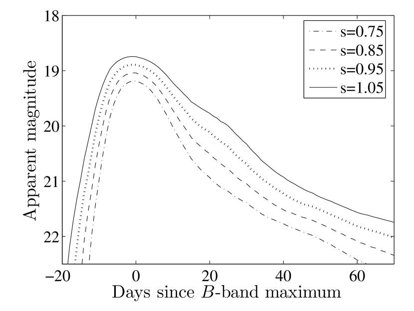
Figure 3.— Examples of template SN Ia light curves with a range of stretch factors, calculated in the WOOTS-clear bandpass. In this example, the light curves are for the cluster Abell 1920, at $z=0.131$. The representative stretch values for SNe Ia in low-$z$ elliptical galaxies are from Sullivan et al. (2006).

4.1.3 Detection Probability

The detection efficiency function described in § 4.1.1 is defined for the magnitude of a point source in a difference image. This means that the interesting quantity in the SN light curve is not its magnitude in a single image, but the magnitude corresponding to the flux difference $\Delta f$ that results from subtracting two epochs from each other. This effective light curve depends on the time that elapsed between the two epochs that are being compared,

$$m_{eff}(t) = ZP-2.5\log(\Delta f)=$$

$$-2.5\log\left(10^{-0.4m(t)}-10^{-0.4m[t+(t_{1}-t_{0})]}\right),$$

where $t$ is the age of the SN, and $t_{0}$ and $t_{1}$ are the times of the template observation and the new observation, respectively.

The detection probability function, $\eta[m_{eff}(t)]$, describes the probability of detecting a SN which occurred $t$ days ago, in a comparison between two epochs.

Since the searches in a given field were not uniformly distributed in time, with some observations conducted close in time to each other, the same SN can, in principle, be discovered in more than one image. For example, when two closely spaced observations were compared to the same template, a SN that was discovered in the first observation (at time $t_{1}$) would simply be rediscovered in the second observation (at time $t_{2}$). To avoid counting such objects twice in our calculation of the visibility time, we assign the second observation a reduced detection efficiency, which describes the probability of detecting only a SN that was not detected in the previous observation. We do this by shifting $\eta(t)$ by $t_{2}-t_{1}$ days, and subtracting from it the combined detection probability (the probability that the SN is discovered in both observations): $\eta_{2}^{*}=\eta_{2}-(\eta_{2}\times\eta_{1}$). In principle, this operation can be repeated for any number of consecutive observations, e.g., for three consecutive observations, $\eta_{3}^{*}$ will be the probability to discover a SN in the third observation ($\eta_{3}$), minus the probabilities of discovering it both in the first observation and in the third one, the second and the third, and in all three observations: $\eta_{3}^{*}=\eta_{3}-(\eta_{3}\times\eta_{2})-(\eta_{3}\times\eta_{1})-(\eta_{3}\times\eta_{2}\times\eta_{1}$). In practice, the temporal distribution of the images does not require considering more than two consecutive observations, i.e., either $\eta^{*}=\eta_{1}$ or $\eta^{*}=\eta_{2}^{*}$ are used in equation 2.

4.2. Cluster Stellar Luminosity

4.3. Aperture Luminosity Measurement

SN rates are often measured relative to the stellar luminosity within the search area, in a particular band. The cluster luminosities in our sample cannot be measured easily from WOOTS data, since they lack color and spectral information from which cluster membership could be determined. Instead, we have used the data from the SDSS DR4 to measure cluster luminosities for 72 clusters, i.e., about one-half of the sample. Unlike traditional cluster stellar luminosity measurements, we do not identify the individual cluster member galaxies from the data. Instead, we have based our measurements on a method similar to aperture photometry, as follows.

The net cluster-galaxy flux is

$$f_{cluster}=k\times(\sum_{i}f_{i}-\pi R_{c}^{2}\overline{f}_{bg}),$$ (5)

where $k$ is the K-correction factor, and the summation is over all galaxies within a cluster radius $R_{c}$ that satisfy the criteria that will be described below. The total Galactic extinction-corrected flux of galaxy $i$ is denoted by $f_{i}$, and $\overline{f}_{bg}$ is the average “background”-galaxy flux per unit area. The net cluster-galaxy flux is translated to luminosity based on the cluster redshift and the appropriate K-correction, and corrected for incompleteness, as described below. In what follows, we describe the derivation of cluster stellar luminosities in the SDSS $r$ band. The luminosities in three other SDSS photometric bands, $g,i,$ and $z$, were measured in the same manner.

To lessen the contamination of our measurements by foreground galaxies, we ignored, both within and outside our apertures, galaxies brighter than the brightest-cluster galaxy (BCG) in each field. The BCG was identified from the SDSS catalog by its magnitude, color, and where available, by redshift. We also ignored galaxies fainter than the SDSS $95\%$ completeness limit (see Table 2).

Table 2Adopted Photometric Parameters

	(1)	(2)	(3)	(4)
band	$m_{lim}$	$M_{{\rm band},\odot}$	$M^{*}$	$\alpha$
	[mag]	[mag]	[mag]
$g$	$22.2$	$5.12$	$-22.01\pm 0.26$	$-1.00\pm 0.06$
$r$	$22.2$	$4.64$	$-22.21\pm 0.05$	$-0.85\pm 0.03$
$i$	$21.3$	$4.53$	$-22.31\pm 0.08$	$-0.70\pm 0.05$
$z$	$20.5$	$4.51$	$-22.36\pm 0.06$	$-0.58\pm 0.04$

Leir & van den Bergh (1977) estimated cluster radii, $R_{LvdB}$, for 1889 Abell clusters, using the red plates of the Palomar Sky Survey, by superposing a grid of circles of various radii on each cluster, and selecting by eye the radius that encompasses most uniformly all visible cluster members. We have examined their estimate for 12 of our clusters, by measuring the net cluster-galaxy flux as described above, as a function of $R_{c}$. We find that the enclosed flux profile generally tends to a constant value (to within errors) at radii $R_{c}\approx R_{LvdB}$, and we therefore adopt $R_{LvdB}$ as the cluster radius of each cluster in our sample. In §3 we investigate the effect of varying the choice of $R_{c}$ between $0.5R_{LvdB}$ and $1.5R_{LvdB}$, according to a normal distribution centered on $R_{LvdB}$ with $\sigma=0.2R_{LvdB}$. We find that this uncertainty in the cluster radius results in a $\sim 1\%$ error in the stellar luminosity.

The average background-galaxy flux per unit area, $\overline{f}_{bg}$, was estimated from the flux per unit area of galaxies that satisfy the above criteria, in an annulus of area of $\sim 0.5$ deg² centered on the cluster, with inner radius of $0.4^{\circ}$. The inner radius is chosen to be large enough to exclude cluster member galaxies, but small enough to be representative of the large-scale structure in the vicinity of the cluster. In order to check whether the measured cluster luminosity is sensitive to the choice of background annulus inner radius, we calculated the luminosity of each cluster using a range of inner radii, between $0.35^{\circ}$ and $0.45^{\circ}$. We experimented with both using a fixed angular radius for all of the clusters, and using a buffer that is proportional to the cluster radius. The luminosities that result from the various methods of background estimation have an rms of $8\%$. We take this uncertainty into account in our error budget (see §5).

To convert the observed magnitudes to rest-frame magnitudes, a K-correction factor was calculated for each cluster assuming that all the cluster light is emitted by elliptical galaxies at the cluster redshift. The net cluster flux was then translated to luminosity, according to the cluster redshift and the adopted cosmology. The faint cut on the galaxy magnitudes means that the summed luminosity includes only galaxies brighter than some limiting luminosity, which depends on the cluster redshift. We correct for this incompleteness by multiplying the summed luminosity by the fraction of light that comes from the faint end of a Schechter (1976) luminosity function:

$$C=\frac{\int_{0}^{\infty}{\Phi(L)dL}}{\int_{L_{lim}(m_{lim},z)}^{\infty}\Phi(L)dL},$$ (6)

where $\Phi(L)dL=\Phi^{*}(L/L^{*})^{\alpha}{\rm exp}(-L/L^{*})d(L/L^{*})$. We adopt $\alpha=-0.85\pm 0.03$ and $M^{*}=-22.21\pm 0.05$ as the mean values for the $r$-band luminosity function parameters in clusters (Goto et al. 2002; see Table 2). The integrated $r$-band luminosity correction factors in our sample are in the range $C-1=0.4^{+0.09}_{-0.07}\times 10^{-3}$ to $8.3^{+1.1}_{-0.9}\times 10^{-3}$, for $z=0.06$ and $z=0.2$, respectively, i.e., always quite small (see Table 3). We note that Goto et al. (2002) excluded the BCGs from the analysis when fitting the data to the Schechter function. We therefore applied the correction above after subtracting the luminosity of the BCG from the summed luminosity, and added the BCG luminosity to the corrected cluster luminosity.

Several recent studies have argued that BCG galaxy luminosities are underestimated in SDSS, because the default sky subtraction algorithm removes the outer, low surface-brightness, flux from these galaxies (Graham et al. 2005; Bernardi et al. 2005; Lauer et al. 2006; Desroches et al. 2006; von der Linden et al. 2006). L.-B. Desroches and C.-P. Ma (private communication) find that, for a subsample of the Miller et al. (2005) C4 sample, improved sky subtraction increases the luminosity by a mean factor 1.3 over the total deVaucoulers SDSS luminosity. For five of our BGCs which are in common with their subsample they find similar correction factors. It is clear that BCG luminosity measurements from the SDSS are indeed sensitive to the sky-level subtraction algorithm. On the other hand, it is not certain that the new corrected measurements are in fact superior, e.g., they might include in the BCG measurement some light from neighboring galaxies. We therefore choose to increase the BCG luminosities by 15%, with an additional systematic uncertainty of $\pm 15\%$. Since the BCG luminosity typically constitutes about 6% of the cluster luminosity, this correction lowers our derived SN rate by 1%, and increases the systematic error in the rate by $\pm 1\%$.

Table 3Measured Cluster Luminosities

Abell	$z$	Luminosity [$10^{12}L_{\sun}$]				Luminosity	Mass
Number		$g$	$r$	$i$	$z$	Correction (r)	[$10^{12}M_{\sun}$]
125	0.19	2.51	2.51	3.10	4.50	1.0071	8.2 $\pm 1.9$
175	0.13	4.67	6.03	7.59	8.52	1.0027	16.3 $\pm 3.8$
279	0.08	0.82	0.91	1.41	1.61	1.0008	5.0 $\pm 1.2$
655	0.12	4.55	5.00	6.99	8.14	1.0025	19.8 $\pm 4.7$
917	0.13	1.04	1.40	1.79	2.15	1.0029	4.2 $\pm 1.0$
924	0.10	0.60	0.83	1.13	1.29	1.0014	2.9 $\pm 0.7$
947	0.18	1.55	2.06	2.32	2.27	1.0061	3.3 $\pm 0.8$
975	0.12	0.87	0.94	1.20	1.66	1.0022	3.3 $\pm 0.8$
1025	0.15	2.81	3.30	3.77	4.77	1.0041	7.3 $\pm 1.7$
1066	0.07	1.60	1.86	2.26	2.71	1.0006	4.8 $\pm 1.1$
1073	0.14	2.27	3.18	3.46	4.56	1.0033	6.2 $\pm 1.5$
1081	0.16	3.41	4.02	5.49	6.23	1.0046	14.4 $\pm 3.4$
1132	0.14	3.74	5.16	6.58	7.53	1.0031	14.8 $\pm 3.5$
1170	0.16	3.83	3.54	4.29	5.04	1.0049	8.8 $\pm 2.1$
1190	0.08	1.25	1.54	2.18	2.70	1.0008	6.8 $\pm 1.6$
1201	0.17	7.05	8.61	9.57	11.26	1.0054	16.1 $\pm 3.8$
1207	0.14	0.80	0.71	0.96	1.59	1.0031	3.5 $\pm 0.8$
1227	0.11	2.45	3.19	4.50	4.65	1.0019	11.5 $\pm 2.7$
1474	0.08	1.17	1.52	1.84	2.12	1.0008	3.7 $\pm 0.9$
1477	0.11	0.08	0.15	0.18	0.24	1.0019	0.4 $\pm 0.1$
1524	0.14	1.77	2.07	2.50	3.12	1.0032	5.4 $\pm 1.3$
1528	0.15	1.34	1.78	2.44	3.22	1.0043	7.5 $\pm 1.8$
1539	0.17	3.15	4.32	5.23	6.76	1.0056	11.7 $\pm 2.8$
1552	0.08	1.95	2.11	2.68	3.30	1.0010	6.4 $\pm 1.5$
1553	0.17	5.46	5.39	6.83	8.30	1.0051	16.1 $\pm 3.8$
1566	0.10	0.75	0.84	1.13	1.44	1.0015	3.2 $\pm 0.8$
1617	0.15	2.60	2.77	3.58	4.62	1.0041	9.3 $\pm 2.2$
1661	0.17	1.44	2.15	2.87	3.36	1.0053	7.4 $\pm 1.7$
1667	0.17	2.15	2.38	2.92	3.69	1.0051	6.6 $\pm 1.6$
1674	0.11	1.56	1.95	2.78	2.95	1.0017	7.5 $\pm 1.8$
1677	0.18	2.36	2.82	3.33	4.17	1.0066	6.9 $\pm 1.6$
1678	0.17	1.88	2.32	2.71	3.23	1.0055	5.2 $\pm 1.2$
1679	0.17	1.89	2.26	2.67	3.32	1.0055	5.4 $\pm 1.3$
1697	0.18	3.20	3.82	5.14	5.96	1.0066	13.2 $\pm 3.1$
1731	0.19	2.42	2.87	3.78	5.16	1.0076	10.9 $\pm 2.6$
1738	0.12	2.27	2.91	3.41	4.83	1.0021	7.8 $\pm 1.8$
1763	0.19	4.01	5.19	6.60	7.63	1.0070	14.9 $\pm 3.5$
1767	0.07	1.28	1.60	1.95	2.70	1.0006	4.8 $\pm 1.1$
1773	0.08	1.35	1.57	2.00	2.25	1.0008	4.4 $\pm 1.0$
1774	0.17	2.46	2.85	3.23	4.65	1.0054	7.0 $\pm 1.6$
1780	0.08	1.39	1.69	2.16	2.31	1.0008	4.6 $\pm 1.1$
1795	0.06	1.56	1.80	2.19	3.48	1.0005	6.1 $\pm 1.4$
1889	0.19	3.11	3.04	4.02	5.06	1.0069	10.8 $\pm 2.5$
1911	0.19	2.71	2.69	3.43	4.04	1.0074	8.0 $\pm 1.9$
1914	0.17	6.01	7.08	8.52	9.98	1.0056	17.1 $\pm 4.0$
1918	0.14	1.45	1.87	2.25	2.68	1.0034	4.6 $\pm 1.1$
1920	0.13	2.55	2.72	3.47	4.68	1.0029	9.2 $\pm 2.2$
1926	0.13	4.46	5.05	6.41	7.98	1.0029	15.5 $\pm 3.6$
1936	0.14	1.42	1.68	2.12	2.51	1.0033	4.8 $\pm 1.1$
1937	0.14	0.63	0.89	1.23	1.80	1.0033	4.2 $\pm 1.0$
1940	0.14	3.67	4.13	4.89	6.30	1.0034	10.4 $\pm 2.5$
1954	0.18	2.31	2.56	3.09	3.73	1.0064	6.5 $\pm 1.5$
1966	0.15	0.84	1.21	1.53	3.09	1.0041	5.9 $\pm 1.4$
1979	0.17	2.24	2.58	3.10	3.54	1.0054	6.1 $\pm 1.4$
1984	0.12	1.24	1.54	1.97	2.32	1.0025	4.6 $\pm 1.1$
1986	0.12	1.33	1.78	1.97	2.52	1.0022	3.6 $\pm 0.8$
1990	0.13	0.89	1.40	1.98	2.28	1.0026	5.6 $\pm 1.3$
1999	0.10	2.61	2.98	3.88	4.70	1.0016	9.7 $\pm 2.3$
2005	0.13	2.21	2.79	3.47	4.01	1.0026	7.4 $\pm 1.7$
2008	0.18	1.28	2.20	2.78	3.74	1.0064	7.2 $\pm 1.7$
2009	0.15	2.73	3.72	4.40	6.00	1.0042	9.9 $\pm 2.3$
2029	0.08	2.49	2.85	3.36	5.62	1.0008	9.2 $\pm 2.2$
2061	0.08	1.72	1.64	2.17	2.09	1.0008	4.4 $\pm 1.0$
2062	0.11	1.99	2.25	2.94	3.56	1.0019	7.4 $\pm 1.8$
2089	0.07	0.51	0.79	0.94	0.84	1.0007	1.4 $\pm 0.3$
2100	0.15	3.03	3.80	4.69	5.78	1.0042	10.5 $\pm 2.5$
2122	0.07	0.68	0.91	1.13	1.44	1.0005	2.7 $\pm 0.6$
2172	0.14	1.21	1.59	1.97	2.55	1.0033	4.7 $\pm 1.1$
2213	0.16	1.15	1.39	1.52	2.05	1.0047	2.8 $\pm 0.7$
2235	0.15	1.45	1.78	2.27	2.64	1.0041	5.2 $\pm 1.2$
2244	0.10	1.83	2.76	3.38	3.31	1.0014	5.9 $\pm 1.4$
2255	0.08	3.64	4.14	5.46	6.00	1.0009	12.7 $\pm 3.0$

4.3.1 Comparison to Other Luminosity Measurements

The reliability of our luminosity measurement method can be tested by comparing our results to independent measurements of the same clusters. The comparison can be particularly straightforward, if the compared luminosities were derived from the same data, namely, the SDSS. Miller et al. (2005) describe their compilation of a cluster catalog, containing $748$ clusters selected spectroscopically from the SDSS database, 12 of which are in our sample and are fully covered by the SDSS DR4. Miller et al. (2005) calculate the $r$-band luminosities of the clusters as the summed luminosities of all galaxies within $2.1$ Mpc (for our choice of $H_{0}$) from the center of the cluster, within 4$\sigma$ in redshift space, and more luminous than $1.4\times 10^{10}L_{\sun}$ (corresponding to a $17.8$ mag galaxy at $z=0.11$). In order to compare our results to theirs, we have calculated the aperture-based luminosities for the $12$ clusters that appear in both samples, with the same radius and limiting luminosity criteria. Excluding Abell 1539, for which the luminosity measurement of Miller et al. was corrupted by a satellite trail in the SDSS $r$-band image, we find that the mean difference between the two measurements of every cluster is $\sim 20\%$.

4.3.2 Measured Luminosities

Table 3 lists our luminosity measurements for the 72 clusters in our sample that are covered by the SDSS DR4 (the “SDSS clusters”). Due to the WOOTS selection criteria (Paper I), the luminosities span a small range, with $68\%$ of the clusters having $L_{r}=2.3^{+1.7}_{-0.9}\times 10^{12}L_{r,\sun}$ (Fig. 4). Within this range, there is no clear trend with other cluster parameters. We therefore assign to the clusters for which we do not have SDSS data (the “non-SDSS clusters”) random luminosities drawn from the luminosity distribution of the SDSS clusters. We estimate the uncertainties in the SN rate due to this random luminosity assignment in § 5.

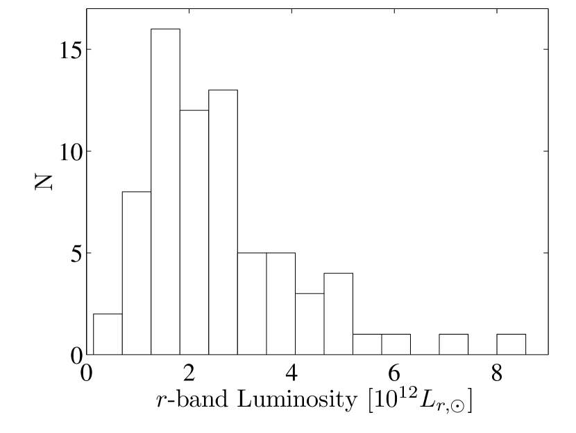
Figure 4.— Distribution of stellar luminosities of the WOOTS clusters that are in the SDSS DR4 (the “SDSS clusters”), as measured with our photometric aperture technique.

The actual luminosity that we require in Eq. 1 is not the total cluster luminosity, but the cluster luminosity included within the search area. For every WOOTS image we define the effective search area as the overlap area between the image and its reference image. The reference image was assigned a zero search area, since the survey was sensitive only to SNe that are brighter in the later epoch (see Paper I). For the SDSS clusters, we calculate the luminosity, as described above, contributed by galaxies that are inside the effective area of an image pair. If the full cluster area within $R_{c}$ is covered by the image (usually clusters with $R_{c}<6^{\prime}$), we adopt the calculated cluster luminosity instead.

To estimate the luminosity inside the search area of the non-SDSS clusters, we need to scale down the cluster luminosity according to the luminosity profile and the effective search area. Figure 5 shows, for the SDSS clusters, the mean fraction of cluster luminosity, $L(<r)/L(<R_{c})$, measured within an aperture of radius $r$, vs. the radius normalized by the cluster radius, $r/R_{c}$. The solid line is a second-order polynomial fit to the data, $L_{r}/L_{R_{c}}=-0.07+1.64r/R_{c}-0.56(r/Rc)^{2}$. We use this relation for all the non-SDSS clusters with $R_{c}>6^{\prime}$, adopting for $r$ the radius of a circle with an area equal to the effective search area of the image. Figure 6 examines the reliability of this approximation. For each SDSS cluster, we estimate the luminosity within a circular aperture with an area of $12^{\prime}\times 12^{\prime}$ (the dimensions of the CCD used in WOOTS), using the above relation, and plot it against the luminosity that is measured directly in the effective search area. The difference between the estimated luminosities and the measured ones has an rms deviation of $16\%$, which we adopt as the uncertainty introduced by this approximation.

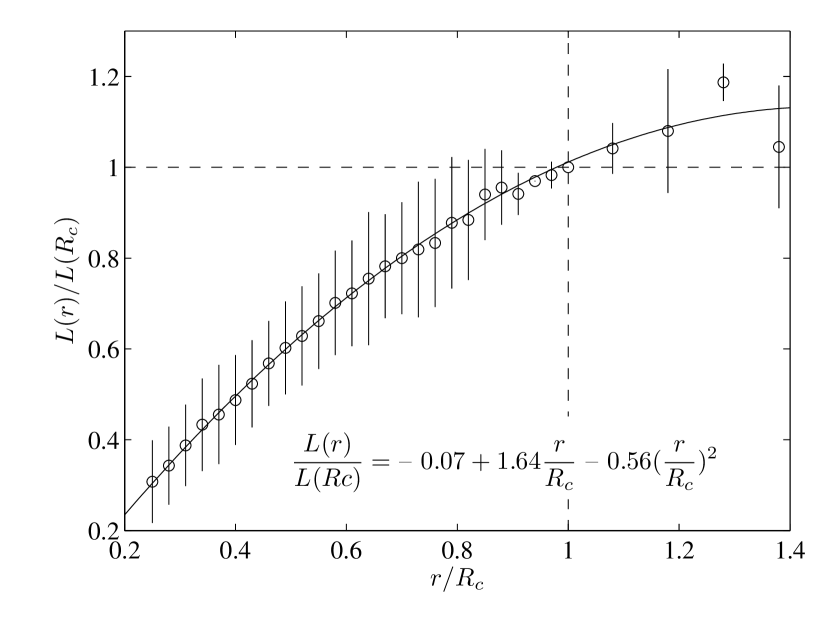
Figure 5.— Composite enclosed cluster-galaxy light profile, based on all SDSS clusters in the sample. Error bars represent the measured rms over the sample. The solid line is the indicated second-order polynomial fit to the data.

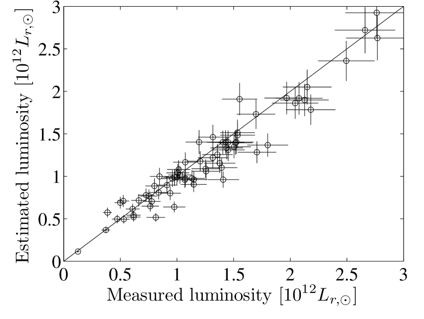
Figure 6.— Comparison between the luminosity within the WOOTS search area, estimated using the relation in Fig. 5, and the actual luminosity measured in the image area, for the SDSS clusters. The solid line represents perfect agreement.

5. Results and Error Estimation

Combining all the elements of the calculation, as described above, we can derive the cluster SN rate and its uncertainty. The dominant source of error in the rate is the Poisson statistics of the (small) number of SNe, $N=6^{+3.58}_{-2.38}$ (68% confidence limit). To determine the propagation of the uncertainties in all the parameters and measurements that enter the rate derivation to the overall systematic uncertainty, we have conducted a Monte Carlo experiment, in which we calculate the SN rate many times, with the parameters drawn at random each time from their respective distributions. The distributions are either Gaussian with an rms deviation set to equal the parameter error, or a specific measured distribution (e.g., the distribution of light-curve stretch factors). The distributions of SN rates from the Monte Carlo simulation permit both a reliable error estimation and a determination of the most probable rate. Because of the nonlinear dependence of the rate on some of the parameters entering the calculation (e.g., stretch factor and luminosity), the most probable SN rate will not necessarily be the SN rate obtained from the combined most-probable values of all the input parameters. We will take as the most probable SN rate the peak of the Monte Carlo distribution, with a systematic error derived directly from this distribution, and a statistical error that originates from the Poisson confidence limits on the number of events.

We have also examined the sensitivity of the SN rate to the uncertainties in the individual parameters, by turning on the Monte Carlo simulation for each one separately. Table 4 summarizes the mean values and the uncertainty in the SN rate, due to each of the parameters.
Luminosity error: The overall luminosity error is about $5\%$, and is dominated by the process of randomly drawing the non-SDSS cluster luminosities from the luminosity distribution of the SDSS clusters. Varying the cluster radius has a much smaller effect, of $\sim 1\%$. Similarly, the uncertainty due to the luminosity gradient of the clusters introduces an SN rate error smaller than $0.2\%$. Varying the inner radius of the background annulus results in an error of less than $0.5\%$.
Visibility time error: The uncertainties in the visibility time measurement have a less intuitive effect on the final rate distribution. The visibility time is most sensitive to the shape and parameters of the efficiency function, mainly $m_{0.5}$, which is the magnitude at which the efficiency drops to half its maximum value. We find that drawing the efficiency parameters from normal distributions centered on their best estimated or mean values results not only in a dispersion in SN rates, but also in an overall decrease in the rate. The reason for this behavior is that the dependence of the rate on the efficiency is nonlinear. A slightly higher efficiency (caused by higher $m_{0.5}$ or lower $s$) will result in a decrease in the SN rate, and vice versa, but for a similar absolute change in the efficiency parameters, the decrease in the rate is larger than the increase in the rate. The same applies to the distribution of SN light-curve stretch factors. Drawing light curves from a stretch-factor distribution, even if it is symmetric about the mean value, causes an overall decrease in the mean SN rate. In our case, all of these effects are, of course, negligible compared to the statistical error. The total systematic error, which in our case is $\sim 6\%$, will become comparable to the statistical error in future surveys with the detection of several hundred SNe.

Table 4Sensitivity of the SN Rate to the Uncertainty in Individual Parameters and Measurements.

Parameter	Parameter distribution	$<SNu_{r}>$	$\sigma$
Non-SDSS cluster-luminosity draw	SDSS cluster	$0.325$	$0.016$
	luminosity distribution
Cluster radius ($R_{c}$)	Normal with $\sigma=20\%$	$0.327$	$0.004$
$L$(in image) $\propto L(<r)$	Normal with $\sigma=0.16$	$0.324$	$0.002$
Background annulus	Measured1; $\sigma=0.07$	$0.3243$	$0.0007$
Overall uncertainty in $L$		$0.327$	$0.017$
ZP (from USNO-B / SDSS)	Normal with $\sigma=0.3/0.04$	$0.316$	$0.004$
$m_{0.5}vs.ZP$	Normal with $\sigma=0.4$	$0.301$	$0.007$
$svs.N_{Res}$	Normal with $\sigma=0.3$	$0.321$	$0.002$
LC stretch factor	From Sullivan et al. (2006b)	$0.318$	$0.004$
Overall uncertainty in visibility time		$0.287$	$0.009$
Overall uncertainty from all parameters		$0.290$	$0.017$

By calculating the luminosity for different buffer selections; see § 4.2

We note that some parameters were not varied in our simulation, since their errors are significantly smaller. (1) The uncertainties in the Schechter luminosity function parameters cause a symmetrical change of $0.16\%$ in the luminosity, in the most extreme case, and were therefore ignored. (2) In the calculation of cluster luminosities, we assumed that all of the cluster light is emitted by elliptical galaxies. However, a small fraction of the light does come from spiral galaxies, which have a different K-correction – it is $0.16$ mag smaller at $z=0.06$, and $0.26$ mag larger at $z=0.2$. To check the effect of this assumption, we calculated the SN rate for the unrealistic case, in which half of the cluster galaxies are Sc galaxies. In the $0.06<z<0.2$ range, individual cluster luminosities increase (at $z<0.115$) or decrease (at $z>0.115$) by no more than $10\%$, relative to the all-elliptical case. The actual distribution of cluster redshifts leads to a $\sim 4\%$ increase in the SN rate. Thus, even in this extreme scenario, the influence on the SN rate is smaller than that of the other sources of systematic error.

The resulting SN rates, as determined from the positions of the peaks of the Monte Carlo distributions, and normalized by stellar luminosity in the $g,r,i$, and $z$ bands are given in Table 5. The rates are given in units of SNu_band, defined as SNe (century $10^{10}L_{{\rm band},\sun}$)^-1. We also express our result in the Johnson $B$ band used traditionally for SN rates, in units of SNu_B, by assuming $B-r=1.078$ mag for elliptical galaxies (as calculated from the template elliptical spectrum of Kinney et al. 1996), $M_{r,\sun}=4.64$ (Blanton et al., 2006), and $M_{B,\sun}=5.47$ (Allen 1976).

Table 5SN Ia Rates

Environment	Redshift	Value 1	Units2	Reference
cluster	$0.06<z<0.2$	$0.351^{+0.210}_{-0.139}\pm 0.020$	SNug	This work
		$0.288^{+0.172}_{-0.114}\pm 0.018$	SNur
		$0.229^{+0.137}_{-0.091}\pm 0.014$	SNui
		$0.186^{+0.111}_{-0.074}\pm 0.010$	SNuz
cluster	$0.06<z<0.2$	$0.36^{+0.22}_{-0.14}\pm 0.02$	SNuB	This work
cluster	$0.18<z<0.37$	$0.39^{+0.59}_{-0.25}$	SNuB	Gal-Yam et al. (2002)
cluster	$0.83<z<1.27$	$0.80^{+0.92}_{-0.41}$	SNuB	Gal-Yam et al. (2002)
E/S0	local	$0.16\pm 0.05$	SNuB	Capellaro et al (1999)
cluster	$0.06<z<0.2$	$0.098^{+0.059}_{-0.039}\pm 0.009$	SNuM	This work
E/SO	local	$0.038^{+0.014}_{-0.012}$	SNuM	Mannucci et al. (2005)
E/SO	$0.2<z<0.75$	$0.053\pm{0.011}$	SNuM	Sullivan et al. (2006)

6. Comparison to Other SN Rate Measurements

Our derived cluster SN rate at $0.06<z<0.19$ can be compared to recent measurements of SN rates both in clusters and in the field. In the field, we compare the rate derived in this work to recent measurements of the SN rate in elliptical galaxies per unit stellar luminosity and per unit mass. Cappellaro et al. (1999) measured a local E/S0 SN Ia rate of $0.16\pm 0.05$ SNu_B, which is consistent with the rate we obtain in this luminosity band, $0.36^{+0.22}_{-0.14}\pm 0.02$ SNu_B. To convert our measurement to SNuM [SNuM = SN (century $10^{10}M_{\sun}$)^-1], we follow Mannucci et al. (2005), who used the mass-to-light ratio derived by Bell et al. (2001) to convert the $K$-band luminosities and $B-K$ colors of the galaxies in their sample to stellar mass. We derive the $r-i$ color of each SDSS cluster from the ratio between its measured $r$-band and $i$-band luminosities, $r-i=-2.5\,{\rm log}_{10}(L_{r}/L_{i})-M_{i,\sun}+M_{r,\sun}$. The stellar mass of each cluster is then estimated from the color-dependent stellar mass-to-light ratio derived by Bell et al. (2003), ${\rm log}_{10}(M_{\sun}/L_{z,\sun})=-0.052+0.923(r-i)$ (see Manucci et al. 2005 for a discussion of the validity of this ratio for our purpose). Finally, we define the stellar mass-to-light ratio of our cluster sample as the total mass divided by the total $z$-band luminosity of the entire sample, $M/L=1.89\pm 0.44M_{\sun}/L_{z,\sun}$, and use it to convert the SN rate from SNu_z to SNuM. The resulting SN rate per unit stellar mass is $0.098^{+0.059}_{-0.039}\pm 0.009$  SNuM. Mannucci et al. (2005) used the SN sample of Cappellaro et al. (1999) to measure the SN rate per unit mass as a function of host-galaxy morphological type. They found a rate of $0.038^{+0.014}_{-0.012}$ (converted from $h=0.75$ to $h=0.70$) SNuM for low-redshift ($z<0.02$) E/S0 galaxies, lower than, but consistent with our result for cluster galaxies at a somewhat higher redshift. We note that some of the E/S0 galaxies monitored by Cappellaro et al. are members of nearby galaxy clusters, and therefore the Mannucci et al. (2005) local rate includes both cluster and field early-type galaxies. A discussion of local rates separated by environment will be presented elsewhere.

Sullivan et al. (2006) measured the SN Ia rate at $0.2<z<0.75$, from $124$ SNe discovered by the Supernova Legacy Survey (SNLS), and studied the SN host properties. Following Mannucci et al. (2005) and Scannapieco et al. (2006), they separated the rate into two components, one proportional to stellar mass, and the other proportional to the star formation rate – $SNR_{Ia}(t)=AM(t)+B\dot{M}(t)$. Their best-fit values are $A=0.053\pm{0.011}$ SNuM, $B=(3.9\pm 0.7)\times 10^{-4}$ SNe yr^-1 (M_☉ yr^-1)^-1. Since the stellar mass in their sample is dominated by the early-type galaxies, and these galaxies have virtually no star formation, the parameter $A$ is essentially the SN rate in E/S0 galaxies. Comparison of the E/S0 SN rates measured by Mannucci et al. (2005) and Sullivan et al. (2006) indicates that the rate may be constant with redshift out to $z\approx 0.5$, although an increase by a factor $\sim 2$ is also consistent within the errors. Our measurement in clusters at an intermediate redshift range is consistent with these two field elliptical rate measurements.

In galaxy clusters, Gal-Yam et al. (2002) measured cluster SN Ia rates per unit stellar $B$-band luminosity of $0.39^{+0.59}_{-0.25}$ SNu_B at $<z>=0.25$ and $0.80^{+0.92}_{-0.41}$ SNu_B at $<z>=0.9$ (converting to our adopted cosmology). These estimates were based on the detection of one cluster SN in the low-redshift bin, and one or two in the high-redshift bin, and consequently, the errors are large. Comparing to our measurement of $0.36^{+0.22}_{-0.14}\pm 0.02$ SNu_B, there is a hint for a slow rise in SN rate with redshift. However, the data are equally consistent, given the large error bars, with a constant rate. More accurate SN rate measurements at high $z$, which are in progress, will elucidate this question.

7. Summary

We have analyzed the data from the WOOTS cluster SN survey (Paper I) to derive the SN Ia rate in $0.06<z<0.19$ clusters, normalized by stellar luminosity and by stellar mass (Table 5). In addition to the sample of six cluster SNe Ia discovered by the survey, our measurement required the determination of two variables – the survey visibility time, and the cluster stellar luminosities, which we determined using the survey data, assisted by SDSS data. We have conducted Monte Carlo simulations that mimic the inhomogeneity in the parameters that enter the rate calculation, and quantify the dependence of the systematic errors on the uncertainty in these parameters. The resulting systematic errors are about an order of magnitude smaller than the Poisson errors due to the small number of SNe that were detected.

We find that the SN rate is similar to the rate found in field elliptical galaxies, both locally and out to $z=0.75$. A comparison to cluster SN rates at higher redshifts is similarly consistent with an unchanging rate, but the large uncertainties in current high-$z$ cluster SN rates can also accommodate a decline in the rate with time. We are in the process of obtaining cluster SN rate measurements at high redshift. The emerging dependence of SN rate on cosmic time and on galaxy environment should provide valuable new insights for astrophysics and cosmology.

References

- Abell et al. (1989) Abell, G. O., Corwin, H. G., Jr., & Olowin, R. P. 1989, ApJS, 70, 1
- Adelman-McCarthy et al. (2006) Adelman-McCarthy, J. K., et al. 2006, ApJS, 162, 38
- Astier et al. (2006) Astier, P., et al. 2006, A&A, 447, 31
- Badenes et al. (2006) Badenes, C., Borkowski, K. J., Hughes, J. P., Hwang, U., & Bravo, E. 2006, ApJ, 645, 1373
- Bahcall (1999) Bahcall, N. 1999 Allen’s Astrophysical Quantities, ed. A. Cox, AIP Press (New York: Springer-Verlag), p. 613
- Barris & Tonry (2006) Barris, B. J., & Tonry, J. L. 2006, ApJ, 637, 427
- Bell et al. (2003) Bell, E. F., McIntosh, D. H., Katz, N., & Weinberg, M. D. 2003, ApJS, 149, 289
- Bertin & Arnouts (1996) Bertin, E., & Arnouts, S. 1996, A&AS, 117, 393
- Blanton & Roweis (2006) Blanton, M. R., & Roweis, S. 2006, astro-ph/0606170
- Branch (1998) Branch, D. 1998, ARA&A, 36, 17
- Cappellaro et al. (1999) Cappellaro, E., Evans, R., & Turatto, M. 1999, A&A, 351, 459
- Chang et al. (2006) Chang, R., Gallazzi, A., Kauffmann, G., Charlot, S., Ivezić, Ž., Brinchmann, J., & Heckman, T. M. 2006, MNRAS, 366, 717
- Dahlen et al. (2004) Dahlen, T., et al. 2004, ApJ, 613, 189
- Desroches et al. (2006) Desroches, L.-B., Quataert, E., Ma, C.-P., & West, A. A. 2006, astro-ph/0608474
- Filippenko (1997) Filippenko, A. V. 1997, ARA&A, 35, 309
- Filippenko (2004) Filippenko, A. V. 2004, in Carnegie Observatories Astrophysics Series, Vol. 2: Measuring and Modeling the Universe, ed. W. L. Freedman (Cambridge: Cambridge Univ. Press), p. 270
- Filippenko (2005) Filippenko, A. V. 2005, in “White Dwarfs: Cosmological and Galactic Probes,” ed. E. M. Sion, S. Vennes, & H. L. Shipman (Dordrecht: Springer), p. 97
- Förster et al. (2006) Förster, F., Wolf, C., Podsiadlowski, P., & Han, Z. 2006, MNRAS, 368, 1893
- Gal-Yam et al. (2002) Gal-Yam, A., Maoz, D., & Sharon, K. 2002, MNRAS, 332, 37
- Gal-Yam et al. (2003) Gal-Yam, A., Maoz, D., Guhathakurta, P., & Filippenko, A. V. 2003, AJ, 125, 1087
- Gal-Yam & Maoz (2004) Gal-Yam, A., & Maoz, D. 2004, MNRAS, 347, 942
- Gal-Yam et al (2006) Gal-Yam, A., Maoz, D., Filippenko, A. V., Guhathakurta, P., 2006, in preparation (Paper I)
- Goto et al. (2002) Goto, T., et al. 2002, PASJ, 54, 515
- Graham et al. (2005) Graham, A. W., Driver, S. P., Petrosian, V., Conselice, C. J., Bershady, M. A., Crawford, S. M., & Goto, T. 2005, AJ, 130, 1535
- Greggio (2005) Greggio, L. 2005, A&A, 441, 1055
- Hamuy et al. (1996) Hamuy, M., et al. 1996, AJ, 112, 2408
- Hamuy et al. (2002) Hamuy, M., et al. 2002, AJ, 124, 417
- Hardin et al. (2000) Hardin, D., et al. 2000, A&A, 362, 419
- Holden et al. (2005) Holden, B. P., et al. 2005, ApJ, 620, L83
- Kinney et al. (1996) Kinney, A. L., Calzetti, D., Bohlin, R. C., McQuade, K., Storchi-Bergmann, T., & Schmitt, H. R. 1996, ApJ, 467, 38
- Lauer et al. (2006) Lauer, T. R., et al. 2006, astro-ph/0606739
- Leibundgut (2001) Leibundgut, B. 2001, ARA&A, 39, 67
- Leir & van den Bergh (1977) Leir, A. A., & van den Bergh, S. 1977, ApJS, 34, 381
- Loewenstein (2006) Loewenstein, M. 2006, astro-ph/0605141
- Madau et al. (1998) Madau, P., Della Valle, M., & Panagia, N. 1998, MNRAS, 297, L17
- Mannucci et al. (2005) Mannucci, F., Della Valle, M., Panagia, N., Cappellaro, E., Cresci, G., Maiolino, R., Petrosian, A., & Turatto, M. 2005, A&A, 433, 807
- Maoz & Gal-Yam (2004) Maoz, D., & Gal-Yam, A. 2004, MNRAS, 347, 951
- Miller et al. (2005) Miller, C. J., et al. 2005, AJ, 130, 968
- Monet et al. (2003) Monet, D. G., et al. 2003, AJ, 125, 984
- Neill et al. (2006) Neill, J. D., et al. 2006, astro-ph/0605148
- Nomoto et al. (1984) Nomoto, K., Thielemann, F.-K., & Yokoi, K. 1984, ApJ, 286, 644
- Nomoto et al. (2005) Nomoto, K., Tominaga, N., Umeda, H., Maeda, K., Ohkubo, T., & Deng, J. 2005, Nuclear Physics A, 758, 263
- Nugent et al. (2002) Nugent, P., Kim, A., & Perlmutter, S. 2002, PASP, 114, 803
- Oke & Sandage (1968) Oke, J. B., & Sandage, A. 1968, ApJ, 154, 21
- Pain et al. (1996) Pain, R., et al. 1996, ApJ, 473, 356
- Pain et al. (2002) Pain, R., et al. 2002, ApJ, 577, 120
- Perlmutter et al. (1999) Perlmutter, S., et al. 1999, ApJ, 517, 565
- Phillips (1993) Phillips, M. M. 1993, ApJ, 413, L105
- Poznanski et al. (2002) Poznanski, D., Gal-Yam, A., Maoz, D., Filippenko, A. V., Leonard, D. C., & Matheson, T. 2002, PASP, 114, 833
- Riess et al. (1998) Riess, A. G., et al. 1998, AJ, 116, 1009
- Riess et al. (2004) Riess, A. G., et al. 2004, ApJ, 607, 665
- Scannapieco & Bildsten (2005) Scannapieco, E., & Bildsten, L. 2005, ApJ, 629, L85
- Schechter (1976) Schechter, P. 1976, ApJ, 203, 297
- Silva & Cornell (1992) Silva, D. R., & Cornell, M. E. 1992, ApJS, 81, 865
- Struble & Rood (1991) Struble, M. F., & Rood, H. J. 1991, ApJS, 77, 363
- Sullivan et al. (2006) Sullivan, M., et al. 2006, astro-ph/0605455
- Tonry et al. (2003) Tonry, J. L., et al. 2003, ApJ, 594, 1
- van Dokkum & Franx (2001) van Dokkum, P. G., & Franx, M. 2001, ApJ, 553, 90
- von der Linden et al. (2006) von der Linden, A., Best, P. N., Kauffmann, G., & White, S. D. M. 2006, astro-ph/0611196
- Wuyts et al. (2004) Wuyts, S., van Dokkum, P. G., Kelson, D. D., Franx, M., & Illingworth, G. D. 2004, ApJ, 605, 677
- Yungelson & Livio (2000) Yungelson, L. R., & Livio, M. 2000, ApJ, 528, 108