Origin of solar torsional oscillations

Abstract

Helioseismology has revealed many details of solar differential rotation and also its time variation, known as torsional oscillations. So far there is no generally accepted theoretical explanation for torsional oscillations, even though a close relation to the solar activity cycle is evident. On the theoretical side non-kinematic dynamo models (including the Lorentz force feedback on differential rotation) have been used to explain torsional oscillations. In this paper we use a slightly different approach by forcing torsional oscillations in a mean field differential rotation model. Our aim is not a fully self-consistent model but rather to point out a few general properties of torsional oscillations and their possible origin that are independent from a particular dynamo model. We find that the poleward propagating high latitude branch of the torsional oscillations can be explained as a response of the coupled differential rotation / meridional flow system to periodic forcing in mid-latitudes, of either mechanical (Lorentz force) or thermal nature. The speed of the poleward propagation sets constraints on the value of the turbulent viscosity in the solar convection zone to be less than $3\times 10^{8}\,\mbox{m}^{2}\,\mbox{s}^{-1}$. We also show that the equatorward propagating low latitude branch is very unlikely a consequence of mechanical forcing (Lorentz force) alone, but rather of thermal origin due to the Taylor-Proudman theorem.

1. Introduction

Solar torsional oscillations have been known to exist for more than two decades. Howard & Labonte (1980) presented the first observations of torsional oscillations using Mt. Wilson Doppler measurements and pointed out the 11 year periodicity and the relation to the solar cycle. These early observations showed only the equatorward propagating branch at low latitudes. The high latitude branch (above $60\arcdeg$), which is in amplitude at least twice as strong as the equatorward propagating branch, was found more recently through helioseismic measurements by Toomre et al. (2000), Howe et al. (2000), Antia & Basu (2001), Vorontsov et al. (2002), and Howe et al. (2005). These inversions also show that the high latitude signal penetrates almost all the way to the base of the convection zone. The depth penetration of the low latitude signal is more uncertain due to the lower amplitude, which is comparable to the uncertainties of the inversion methods in the lower half of the convection zone. The most interesting feature of the low latitude branch is an inclination of the phase with respect to the rotation axis by about $25\arcdeg$. This inclination is very close to the inclinations of the isorotation contours of $\Omega$ as pointed out by Howe et al. (2004).

On the theoretical side a variety of explanations have been proposed: macroscopic Lorentz force feedback, microscopic Lorentz force feedback, and thermal forcing.

The idea of macroscopic Lorentz force feedback (computed from the large scale magnetic mean field of the solar dynamo) was originally proposed by Schüssler (1981) and Yoshimura (1981) and has been incorporated into dynamo models more recently by Covas et al. (2000, 2004, 2005). While these models address the non-linear Lorentz force feedback using a simplified equations of motion (considering only the longitudinal component), models by Jennings (1993) and Rempel (2006) consider the Lorentz force feedback also in the meridional plane. The model of Rempel et al. (2005), Rempel (2006) is along the lines of the $\alpha\Lambda$-models by Brandenburg et al. (1990, 1991, 1992), Moss et al. (1995), and Muhli et al. (1995) (coupling mean field models for differential rotation, meridional flow and magnetic field evolution), but puts more emphasis on the role of the meridional flow leading to a flux-transport dynamo (see e.g. Dikpati (2005) for a recent review on the development of flux-transport dynamos).

Microscopic Lorentz force feedback (quenching of turbulent transport processes driving differential rotation ’$\Lambda$-quenching’) has been addressed by Kitchatinov & Pipin (1998), Kitchatinov et al. (1999), and Küker et al. (1999).

Very recently Spruit (2003) proposed a thermal origin of the low latitude branch of torsional oscillations, driven through enhanced radiative losses in the active region belt. This theory also predicts an inflow into the active region belt, which has been observed by Komm et al. (1993), Komm (1994), and Zhao & Kosovichev (2004).

The investigation presented here is based on the model of Rempel (2006); however we take a different approach by decoupling the excitation of torsional oscillations from a detailed dynamo model. We use the differential rotation model of Rempel (2005) and force torsional oscillations through mechanical and thermal perturbations to address the question of what type of forcing is required to get a response comparable to the observed torsional oscillations.

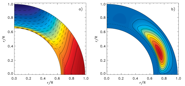
Figure 1.— a) Differential rotation (solid contours correspond to faster rotation, dashed contours to slower rotation than the core of the sun); b) Stream function of meridional flow (solid contours correspond to a counter clockwise flow). The amplitude of differential rotation is $30\%$ of the core rotation rate, the amplitude of the meridional flow is $11\,\mbox{m}\,\mbox{s}^{-1}$ ($2\,\mbox{m}\,\mbox{s}^{-1}$) at the top (bottom) of the convection zone.

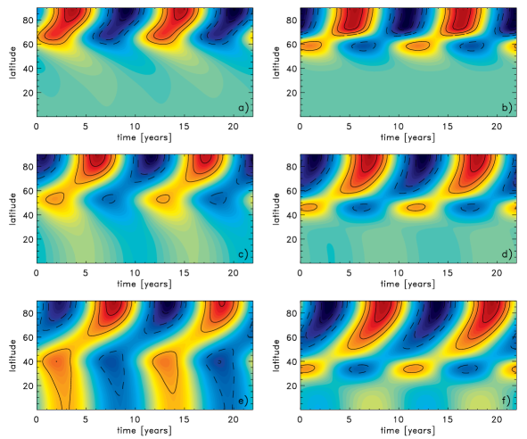
Figure 2.— Torsional oscillations produced by periodic perturbations at a fixed location. The left panels (a, c, e) show the response to a periodic perturbation in the angular velocity (mechanical forcing), the right panels (b, d, f) the response to a periodic perturbation in entropy (thermal forcing). Closed contours correspond to positive values (faster rotation), dashed contours to negative values (slower rotation). From top to bottom the position of the perturbation in latitude is varied between $60\arcdeg$ (a, b), $45\arcdeg$ (c, d), and $30\arcdeg$ (e, f). In all cases the strongest signal is found at the pole, independent from the location of the forcing. The power on the poleward side is always higher than on the equatorward side.

We emphasize that this is not a fully self-consistent explanation of torsional oscillations since we do not incorporate a full dynamo model also considering the non-linear feedback of zonal and meridional flow variations on the magnetic field evolution. We have published such a self-consistent non-linear dynamo model (based on a flux-transport dynamo and the same differential rotation model we use in this paper) in Rempel (2006). We found that many features of torsional oscillations discussed in that paper are more general, meaning independent from a particular dynamo model. The goal of this paper is to point out these general properties that are strongly related to influence of the Taylor-Proudman theorem on amplitude and phase of torsional oscillations.

2. Model

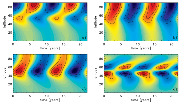
Figure 3.— Influence of viscosity and meridional flow on the poleward propagation of zonal flow variations. Panels a) and b) compare to models different values of the turbulent viscosity: a) $\nu_{t}=3\times 10^{8}\,\mbox{m}^{2}\,\mbox{s}^{-1}$ and b) $\nu_{t}=1.2\times 10^{9}\,\mbox{m}^{2}\,\mbox{s}^{-1}$. A higher value of the turbulent viscosity leads to a faster poleward propagation of the flow pattern. Both cases show the response to a periodic mechanical forcing at $45\arcdeg$ latitude. Panel c) shows the same model as panel a), however, the meridional is not allowed to change in response to the zonal flow variation. In this case the maximum amplitude coincides with the location of the forcing region and the velocity of the poleward propagation of the signal is reduced. Panel d) shows the variation of meridional flow pattern (the reference state meridional flow is subtracted) associated with poleward moving zonal flow pattern shown in Panel a). The amplitude of the meridional flow variation is around $0.2\,\mbox{m}\,\mbox{s}^{-1}$ for a solar like zonal flow variation of around $4$ nHz at the pole.

Our theoretical analysis is based on the differential rotation model developed by Rempel (2005). This model is an axisymmetric mean field model incorporating a parametrization of turbulent angular momentum transport ’$\Lambda$-effect’ (Kitchatinov & Rüdiger 1993). We refer to Rempel (2005) for details of this model. For this investigation we use a reference model close to the model used in Rempel (2006), with the minor difference of using a larger value of $\delta=-3\times 10^{-5}$ for the superadiabaticity in the overshoot region (leading to more solar like differential rotation in terms of inclination of the isorotation contours). Figure 1 shows the differential rotation and the meridional flow stream function for the reference model.

Torsional oscillations can be driven in general through mechanical forcing (Lorentz force) or thermal forcing (pressure imbalances drive geostrophic flows in a rotating system). Most investigations so far focused on the role of the longitudinal Lorentz force, neglecting azimuthal components. This can be partially justified by the fact that the toroidal field is significantly stronger than the poloidal field in an $\alpha\Omega$ dynamo, leading also to a dominant component of the Lorentz force in the longitudinal direction. The azimuthal component could be important for explaining (observed) deviations from the Taylor-Proudman state through a magnetostrophic balance; however, as we show later, this is unlikely to happen in the bulk of the convection zone. Thermal forcing is very efficient in that reproducing the observed amplitude requires only temperature fluctuations of a few tenth of a degree, which can be derived from a geostrophic balance. Assuming a latitudinal balance between Coriolis force and pressure force gives:

$$\Omega_{0}\Omega_{1}r^{2}\sin(2\theta)=\frac{1}{\varrho}\frac{\partial p}{\partial\theta}\approx\frac{1}{\varrho}\frac{\Delta p}{\Delta\theta}\approx\frac{p}{\varrho T}\frac{\Delta T}{\Delta\theta}\;,$$ (1)

which leads to

$$\Delta T\approx\Delta\theta\left(\Omega_{0}r\right)^{2}\sin(2\theta)\left(\frac{\Omega_{1}}{\Omega_{0}}\right)\left(\frac{R}{\mu}\right)^{-1}\;.$$ (2)

Here $\Omega_{0}$ denotes the reference state rotation rate, $\Omega_{1}$ the perturbation (torsional oscillation), $R$ is the gas constant, $\mu$ the mean molecular weight, $r$ the radius, and $\theta$ the co-latitude. Adopting solar values of $\Omega_{0}=2.7\times 10^{-6}\,\mbox{s}^{-1}$, $r=7\times 10^{8}\,\mbox{m}$, $\mu=0.62$, $\Delta\theta=10\arcdeg$ (width of active region belt) and $\Omega_{1}/\Omega_{0}\sim 0.005$, we get

$$\Delta T\sim 0.25\,\mbox{K}\;.$$ (3)

This value is consistent with the temperature perturbation of $0.1$ to $0.2$ K Rempel (2006) imposed in their model to drive the low latitude branch of torsional oscillations. We emphasize that the total temperature perturbation is nearly independent of depth for a fixed torsional oscillation amplitude, meaning that the relative perturbation close to the surface is around $5\times 10^{-5}$ (the same value was given by Spruit (2003)), but only around $10^{-7}$ close to the base of the convection zone.

The following questions will be addressed in this investigation:

1. Are torsional oscillations of thermal or mechanical origin?

2. Are they a consequence of traveling or periodic perturbations in the solar convection zone?

We focus our discussion separately on the high latitude and low latitude branch for reasons that will become more evident in the following discussion.

3. High latitude branch

The high latitude branch has a larger amplitude than the low latitude branch and is propagating poleward, while the low latitude branch is clearly following the equatorward propagating magnetic activity belt. This leads to the fundamental question of whether the poleward branch is also associated with a poleward propagating magnetic pattern at the base of the convection zone (as it has been seen in many interface dynamos), which is not visible at the solar surface. We cannot rule out such a possibility here, but we will show that this is not conclusive and the poleward propagation can be explained as a response of the coupled differential rotation meridional flow system to a non-traveling periodic perturbation in mid-latitudes. To demonstrate this, we incorporate in the differential rotation model a mechanical (in the equation for $\Omega$) or thermal (in the entropy equation) forcing term of the form

$$\frac{\partial\Omega_{1}}{\partial t} = \ldots+A_{\Omega}f(r,\theta)\sin(\omega_{c}t)$$ (4)

$$\frac{\partial s_{1}}{\partial t} = \ldots+A_{s}f(r,\theta)\sin(\omega_{c}t)\;.$$ (5)

Here $\omega_{c}$ corresponds to a $11$ year periodicity (as observed for torsional oscillations), $A_{\Omega}$ and $A_{s}$ are the amplitudes of the forcing, and $f(r,\theta)$ is a Gaussian profile of the form:

$$f(r,\theta)=\exp\left[-\left(\frac{r-r_{0}}{\Delta r}\right)^{2}\right]\cdot\exp\left[-\left(\frac{\theta-\theta_{0}}{\Delta\theta}\right)^{2}\right]\;.$$ (6)

We use for all following models the parameters $r_{0}=0.85\,R_{\odot}$, $\Delta r=0.05\,R_{\odot}$, $\Delta\theta=0.125$, and vary the co-latitude between $\pi/6$, $\pi/4$, and $\pi/3$. For the results presented here the amplitudes $A_{\Omega}$ and $A_{s}$ are of secondary concern (as long as $\Omega_{1}\ll\Omega_{0}$). We have chosen values leading to torsional oscillations of a few percent of the rotation rate.

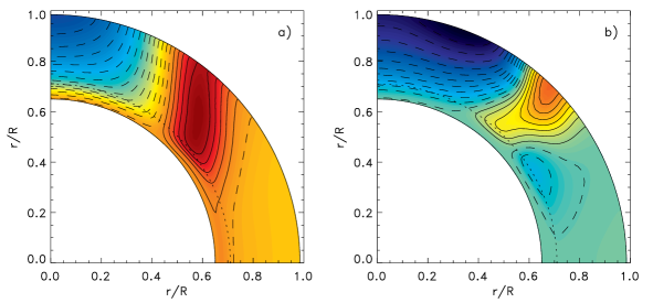
Figure 4.— Snapshots of the torsional oscillations caused by mechanical forcing (left) and thermal forcing (right). The snapshots correspond to $t=0$ years in Fig. 2. Torsional oscillations caused by thermal forcing have the tendency to show stronger deviations from the Taylor-Proudman state.

Figure 2 shows on the left side models with mechanical forcing and on the right side models with thermal forcing. From top to bottom, the latitude of the forcing is varied between $60\arcdeg$, $45\arcdeg$, and $30\arcdeg$. Independent of the nature of the periodic forcing, all models show a strong poleward propagating pattern and a very weak equatorward propagating pattern away from the latitude at which the forcing is applied. The equatorward pattern increases in amplitude when the location of the forcing is moved closer to the equator. The pattern typically shows two peaks, one close to the latitude of the forcing and one right at the pole (with larger amplitude). Comparing the latitudinal extent of the pattern on the polar side of the forcing region with observations, a forcing location in mid-latitudes seems most reasonable.

The time for the signal to travel from about $60\arcdeg$ to the pole is $3$ to $4$ years, which is close to the observed propagation speed. It turns out that the travel time is primarily affected by the turbulent viscosity assumed in the reference model, which is shown in Figure 3. To this end we compare two models with the viscosity values of $3\times 10^{8}\,\mbox{m}^{2}\,\mbox{s}^{-1}$ (panel a) and $1.2\times 10^{9}\,\mbox{m}^{2}\,\mbox{s}^{-1}$ (panel b). We have adjusted in each model the amplitude and the direction of the turbulent angular momentum transport ($\Lambda$-effect) such that the differential rotation and meridional flow remain roughly unchanged. The propagation time for the signal drops from around $3$ to $1$ year when the turbulent viscosity is increased by a factor of $4$. Since solar observations show a time delay of $3$ to $4$ years, this sets constraints on the value of the turbulent viscosity. In our model we get the best fit for values $\lesssim 3\times 10^{8}\,\mbox{m}^{2}\,\mbox{s}^{-1}$. This value is around one order of magnitude smaller than mixing-length estimates for the solar convection zone, it agrees however with the results of Kitchatinov et al. (1994) taking into account rotational quenching of turbulent viscosity. Panel c) shows the same model as panel a) but the meridional flow is not allowed to change in response to the zonal flow variation (we solve only the equation for $\Omega_{1}$ and keep the meridional flow fixed). This leads to a significantly different flow pattern: the maximum amplitude is found close to the forcing region and the propagation of the signal toward the pole slows down. In this way the variation of the meridional flow has a significant influence on the structure of the torsional oscillation pattern. Interestingly, the meridional flow of the reference state is not important, only the induced flow variation. Constructing a model with the same value of the turbulent viscosity, but a different meridional flow, leads to a nearly identical zonal flow pattern (difference in the $1\%$ range). Panel d) shows the meridional flow variation associated with the poleward moving zonal flow pattern shown in panel a). A solar like amplitude of around $4$ nHz for the torsional oscillation leads to a meridional flow variation of around $0.2\,\mbox{m}\,\mbox{s}^{-1}$.

To our knowledge this is so far the only way to constrain the turbulent viscosity directly by observations, without having to relate it to the magnetic diffusivity by making assumptions about the magnetic Prandtl number. We emphasize that our model assumes a constant value throughout the convection zone. In models with a depth dependent viscosity the above mentioned value should reflect more the values in the lower half of the convection zone rather than the surface layers, since they contribute more to the angular momentum transport due to their larger density.

From the results shown in Figure 2 it is difficult to judge whether it is possible to distinguish between a mechanical or thermal forcing. Figure 4 shows meridional cross-sections of the zonal flow pattern. The most obvious difference here is that the mechanical forcing leads to torsional oscillations more aligned with the rotation axis (Taylor-Proudman theorem), while thermal forcing shows a tendency to produce more radially aligned patterns. Beside aligning structures with the rotation axis, the Taylor-Proudman constraint also leads to an almost constant amplitude within the convection zone, while in the case of thermal forcing the entropy perturbations allow for more variation of the amplitude as function of depth.

In the case of the high latitude branch the observations are not detailed enough to distinguish between thermal and mechanical forcing (this may be because in high latitudes the radial direction almost coincides with the axis of rotation). We will show in the next section that there is a significant difference between mechanical and thermal forcing effects in low latitudes.

4. Low latitude branch

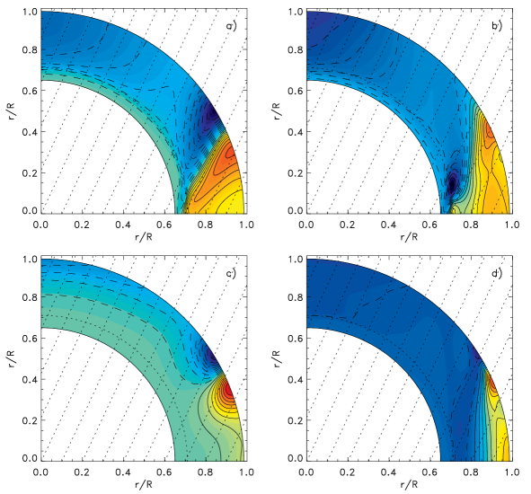
Figure 5.— Mechanical forcing of low latitude zonal flow variations. Panels a) and c) show the forced zonal flow considering no change of the meridional flow (solving the equation for $\Omega_{1}$ for the fixed reference state flow), while panels b) and d) show the zonal flow solving the full system. Panels a) and b) use a forcing function with $r_{0}=0.75\,R_{\odot},\theta_{0}=80\arcdeg$, c) and d) with $r_{0}=0.95\,R_{\odot},\theta_{0}=65\arcdeg$. While panels a) and c) show a zonal flow that closely resembles the properties of the forcing function [especially the $25\arcdeg$ inclination in panel a)], the results shown in panels b) and d) are strongly influenced by rotation. The flow pattern becomes strongly aligned with the axis of rotation and also the amplitude of the zonal flow band with slower rotation is significantly smaller than the faster zonal band.

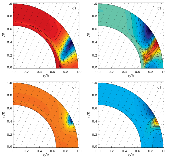
Figure 6.— Thermal forcing of low latitude zonal flow variations. The panels a) and c) show the imposed entropy perturbation, the panels b) and d) the resulting zonal flows. Panels a) and b) use a forcing function with $r_{0}=0.75\,R_{\odot},\theta_{0}=80\arcdeg$, c) and d) with $r_{0}=0.95\,R_{\odot},\theta_{0}=65\arcdeg$. Contrary to the results presented in Figure 5 for mechanical forcing, the driven zonal flows show significant deviations from the Taylor-Proudman state. Especially in panel b) the imposed $25\arcdeg$ angle of the thermal forcing function is clearly visible in the zonal flow field. Also both zonal bands (faster and slower one) are visible, with the faster band on the equatorial side being of larger amplitude and more confined.

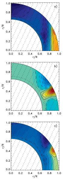
Figure 7.— Combination of mechanical and thermal forcing: a) pure mechanical forcing, b) pure thermal forcing, c) combination of both. The mechanical and thermal forcing functions used here have a radial alignment and the amplitude of the zonal flow in a) and b) is roughly the same. The combination of both forcings produces roughly a $25\arcdeg$ inclination as observed in the solar case.

The most striking feature of the low latitude branch is the systematic deviation from the Taylor-Proudman state. As first pointed out by Howe et al. (2004), the lines of constant phase show an inclination of $25\arcdeg$ to the axis of rotation, similar to the isorotation contours of the differential rotation. We present here a few idealized experiments to differentiate between possible mechanical and thermal forcing. To this end we construct a mechanical forcing function and a cooling function that has a $25\arcdeg$ inclination angle with respect to the axis of rotation. For reasons of simplicity we apply here a stationary perturbation for a time interval of a few month to illustrate the effect. The forcing functions are given by:

$$\frac{\partial\Omega_{1}}{\partial t} = \ldots+A_{\Omega}\,g(r,\theta)\left[\theta-\zeta(r)\right]$$ (7)

$$\frac{\partial s_{1}}{\partial t} = \ldots+A_{s}\,g(r,\theta)\;,$$ (8)

with

$$g(r,\theta) = 0.5\left[1+\tanh\left(\frac{r-r_{0}}{\Delta r}\right)\right]$$ (9)

$$\cdot\exp\left[-\left(\frac{\theta-\zeta(r)}{\Delta\theta}\right)^{2}\right]\,.$$

The function $\zeta(r)$ specifies the inclination of the forcing with respect to the rotation axis. Assuming that $\theta_{0}$ is the location of the forcing at $r_{0}$ and $\lambda$ is the inclination angle we get:

$$\zeta(r)=\lambda+\arcsin\left[\frac{r_{0}}{r}\sin(\theta_{0}-\lambda)\right]\;.$$ (10)

Here $\theta_{0}$ determines the co-latitude of the perturbation at the radius $r_{0}$, where $r_{0}$ marks the depth at which the forcing decreases to half of the convection zone value. We use in the following discussion common values of $\Delta r=0.05\,R_{\odot}$, $\lambda=25\arcdeg$, and $\Delta\theta=0.1$ ($\Delta\theta=0.05$) for mechanical (thermal) forcing, respectively.

To compare results for forcing functions extending through the entire convection zone with those from surface forcing functions, we will use in both cases the parameters $r_{0}=0.75\,R_{\odot},\theta_{0}=80\arcdeg$ (co-latitude); and $r_{0}=0.95\,R_{\odot},\theta_{0}=65\arcdeg$. The amplitudes $A_{\Omega}$ and $A_{s}$ are chosen so that applying the forcing for a time interval of about $4$ months leads to an amplitude of the zonal flow of a few nHz. All results shown in the following discussion show the zonal flow after $4$ months of mechanical or thermal forcing.

The forcing function for the mechanical forcing Eq. (7) is multiplied by the term $\left[\theta-\zeta(r)\right]$ in order to produce a perturbation that has a faster zonal flow equatorward and slower zonal flow poleward of the region the forcing is applied. In the case of the thermal forcing this is not required, since the response to a cooling automatically leads to the formation of two geostrophic flows with opposite directions.

Figure 5 summarizes the results obtained with mechanical forcing, Figure 6 the results from thermal forcing. In the case of mechanical forcing the zonal flows do not resemble the properties of the forcing function (especially the $25\arcdeg$ inclination) unless meridional flow variations are completely suppressed as shown in Figure 5a) and c). If meridional flow variations are considered, the zonal flow pattern shows strong influence of rotation, aligning the pattern with the axis of rotation (Taylor-Proudman theorem). As a consequence, the resulting flow is entirely dominated by the influence of rotation and does not resemble the properties of the applied forcing function. Since the pattern has the tendency to spread parallel to the axis of rotation, a perturbation traveling at the base of the convection zone ($r=0.72\,R_{\odot}$) from $30\arcdeg$ latitude toward the equator, would produce close to the surface a pattern moving from around $40\arcdeg$ to $20\arcdeg$ and could therefore not explain the observed low latitude branch of the observed torsional oscillations. Even applying the forcing close to the surface does not lead to a reasonable flow pattern as shown in Figure 5d).

This result is not too surprising, since adding a forcing in the $\phi$ direction does not impact the meridional force balance that leads to the Taylor-Proudman state. This raises the question if additional magnetic stresses in the meridional plane could cause a deviation from the Taylor-Proudman state as observed (magnetostrophic balance). In a typical $\alpha\Omega$-model for the solar dynamo, the poloidal field is at least a factor of $100$ weaker than the toroidal field. Having a toroidal field strength of around $1$ T ($10$ kG) (Rempel 2006), this yields around $0.01$ T ($100$ G) for the poloidal field. An estimate similar to Eq. (1) leads in the case of a magnetostrophic balance to

$$B_{p}^{2}\approx\mu_{0}\varrho\Delta\theta\left(\Omega_{0}r\right)^{2}\sin(2\theta)\left(\frac{\Omega_{1}}{\Omega_{0}}\right)\;.$$ (11)

Here we assumed that the $\theta$-component of the Lorentz force can be estimated as $B_{p}^{2}/(\mu_{0}\,r\,\Delta\theta)$, where $B_{p}$ denotes the poloidal field strength. Adopting solar values of $\Omega_{0}=2.7\times 10^{-6}\,\mbox{s}^{-1}$, $r=7\times 10^{8}\,\mbox{m}$, $\Delta\theta=10\arcdeg$, $\Omega_{1}/\Omega_{0}\sim 0.005$, and we get

$$B_{p}\approx 1\,\mbox{T}\sqrt{\frac{\varrho}{\varrho_{\rm bc}}}\;,$$ (12)

where $\varrho_{\rm bc}=200\,\mbox{kg}\,\mbox{m}^{-3}$ denotes the density at the base of the convection zone. These values indicate that a magnetostrophic balance is very unlikely in the bulk of the convection zone, but very close to the surface, where the density is very low, it cannot be ruled out (for a typical solar model we have $\varrho\approx 10^{-2}\varrho_{\rm bc}$ at $r=0.98\,R_{\odot}$ and $\varrho\approx 10^{-4}\varrho_{\rm bc}$ at $r=0.997\,R_{\odot}$). There are additional terms of the Lorentz force in the meridional plane that include the much stronger toroidal field: the gradient of the magnetic pressure and magnetic tension force arising from spherical geometry $\sim B_{\phi}^{2}/r$. The latter can lead to a prograde jet within the magnetized region as discussed by Rempel et al. (2000) and Rempel & Dikpati (2003), but not to a flow pattern with two opposite flows on both sides of the active region belt.

In order to address the influence of magnetic pressure, we show in Eq. (13) the $\phi$ component of the vorticity equation considering a stationary flow and neglecting viscous stresses (we also neglect here the magnetic tension force for the reason mentioned above):

$$r\sin\theta\frac{\partial\Omega^{2}}{\partial z}=\frac{g}{\gamma r}\frac{\partial}{\partial\theta}\left(s_{1}+\frac{p_{m}}{p_{0}}\right)$$ (13)

Note that this equation addresses the deviation of the full differential rotation from Taylor-Proudman state. Therefore $s_{1}$ also contains entropy perturbations associated with the reference state differential rotation. Writing $\Omega=\Omega_{r}+\Omega_{t}$ and $s_{1}=s_{r}+s_{t}$, where the subscript ’r’ refers to the reference state and the subscript ’t’ to the torsional oscillation part, we get in leading order:

$$2\,r\sin\theta\left(\Omega_{r}\frac{\partial\Omega_{t}}{\partial z}+\Omega_{t}\frac{\partial\Omega_{r}}{\partial z}\right)=\frac{g}{\gamma r}\frac{\partial}{\partial\theta}\left(s_{t}+\frac{p_{m}}{p_{0}}\right)$$ (14)

Here the first term on the left hand side is the dominant one (typically at least a factor of $5$ larger than the second one for the examples discussed here), relating directly the $z$ derivative of $\Omega_{t}$ to the entropy perturbation and magnetic pressure. Therefore, if the right hand side of Eq. (14) is zero, the torsional oscillation pattern has to be very close to the Taylor-Proudman state with $\partial\Omega_{t}/\partial z=0$. The occurrence of $s_{t}$ together with $p_{m}/p_{0}$ means that a toroidal magnetic field with neutral magnetic buoyancy does not lead to any deviation from the Taylor-Proudman state. If magnetic buoyancy is not compensated, magnetic pressure causes a flow pattern with two opposite flows on both sides of the active region belt; however, they would have the wrong sign (fast moving band on poleward side, slow moving on equatorward side; see also the discussion in next paragraph) when we make the reasonable assumption that the active region belt has a higher magnetic pressure than the surrounding region. We will show in the following paragraph that a reasonable flow perturbation results from the assumption that the active region belt has lower gas pressure, which can be the consequence of a thermal perturbation.

The zonal flow presented in Figure 6b) shows the $25\arcdeg$ inclination angle imposed through the thermal forcing function. Even though the forcing function is symmetric with respect to the latitude of the maximum (given by $\theta=\zeta(r)$), the resulting zonal flows show a significant asymmetry, with the equatorward faster rotating band more confined than the poleward slower rotating band. This is a consequence of the fact that Eq. (13) considers the radial and the latitudinal component of the Coriolis force together. The relative contribution of both components depends on the latitude. In high latitudes we have $\partial/\partial z\sim\partial/\partial r$, resulting in a symmetric flow pattern with the slower rotating band poleward and the faster rotating band equatorward, while in low latitudes we have $\partial/\partial z\sim-\partial/\partial\theta$ leading to a solution $\Omega_{t}\sim-s_{t}$, showing only a fast rotating band centered around the cooling region. In mid-latitudes the solution is a combination of both, with having a stronger fast rotating band that is also more close to the center of the cooling region. Applying the thermal forcing only to the surface, as shown Figure 6d), produces a zonal flow perturbation that is much more confined to the surface; the $25\arcdeg$ inclination is less visible in this case.

This study shows that it is much easier to produce a zonal flow pattern with the observed properties of the low latitude torsional oscillations through thermal forcing rather than mechanical forcing, but it does not explain the observed $25\arcdeg$ inclination angle, since this angle has to be imposed on the thermal forcing function. This could be a consequence of anisotropic thermal heat diffusivity that is larger parallel than perpendicular to the axis of rotation (Kitchatinov et al. 1994). A thermal signal imposed at the surface, as suggested by Spruit (2003), would therefore not penetrate radially into the convection zone but rather in an angle more aligned with the rotation axis. Another possible explanation could be a combination of mechanical and thermal forcing. To illustrate this, we computed in Figure 7 a zonal flow resulting from both types of forcing. Panel a) shows the result of the mechanical forcing alone, panel b) the result of the thermal forcing. In both cases we used $r_{0}=0.9\,R_{\odot}$ and $\theta_{0}=25\arcdeg$. The forcing functions show a radial alignment ($\zeta(r)=\theta_{0}={\rm const.}$). The amplitude of the zonal flow in a) and b) is roughly the same. Applying mechanical and thermal forcing together results in a zonal flow with roughly $25\arcdeg$ inclination with respect to the axis of rotation.

In this section we focused entirely on static forcing functions, not addressing the equatorward propagation of the signal in the course of the solar cycle. This could be easily addressed by incorporating a time dependent phase into Eq. (10); however, this does not impact the conclusions of this section concerning the importance of the Taylor-Proudman theorem, since the timescale for the establishment of the Taylor-Proudman state is significantly shorter than the solar cycle.

5. Discussion

We present in this paper a series of numerical experiments addressing the question of what type of forcing is required to produce a zonal flow variation showing the properties of the observed solar torsional oscillations. Since this study is independent from a specific dynamo model, we can infer a few general conclusions about torsional oscillations and their possible origin:

1. The Taylor-Proudman theorem applies also to perturbations of $\Omega$. Therefore it is crucial to solve in models addressing the origin of torsional oscillations the full momentum equation, including variations of the meridional flow.

2. Mechanically forced zonal flows always have the tendency to spread through the entire convection zone parallel to the axis of rotation.

3. Significant deviations from the Taylor-Proudman state (as observed in low latitudes) require thermal perturbations. A pure mechanical origin of the low latitude torsional oscillations is very unlikely.

4. The fact that the phase of the torsional oscillation signal in low latitudes is inclined such that the signal occurs for a fixed latitude at the base of the convection around 2 years prior to the surface signal does not indicate necessarily that the origin has to be at the base of the convection zone. This is a consequence of the influence of rotation.

5. The high latitude branch of torsional oscillations does not require a forcing propagating poleward in the course of the solar cycle. A poleward propagating zonal flow pattern is the natural response of the coupled differential rotation / meridional flow system to a periodic forcing (mechanical or thermal) in mid-latitudes.

6. The poleward propagation speed of the torsional oscillation pattern is only determined by the value of the turbulent viscosity of the reference model. Best agreement is found for values of $\nu_{t}$ less than $3\times 10^{8}\,\mbox{m}^{2}\,\mbox{s}^{-1}$.

In this paper we did not consider the physical origin of the imposed mechanical or thermal forcings. Possible physical explanations for the forcings considered in this paper are the following:

Macroscopic Lorentz force:

Recently Rempel (2006) showed that the macroscopic Lorentz force in a flux transport dynamo leads to a periodic source in mid-latitudes, where the poloidal magnetic field is sheared by the differential rotation while getting transported downward by the meridional flow. The model provides a poleward propagating branch with the correct amplitude and phase relation to the magnetic cycle. Unlike some of the processes listed below, this type of feedback is unavoidable for a dynamo that is energetically driven through differential rotation. Rempel (2006) showed that the amplitude of the solar torsional oscillations is consistent with a dynamo that converts around $0.1\%\,L_{\odot}$ of energy and produces around $15$ kG of toroidal field at the base of the convection zone.

A different model was presented recently by Covas et al. (2000, 2004, 2005). Their model uses the observed solar rotation profile and allows for perturbations around this profile by considering the longitudinal component of the macroscopic Lorentz force, while the azimuthal component of the momentum equation is neglected (no meridional flow is considered). Their results show torsional oscillations with both branches driven by the Lorentz force that have a remarkable agreement with observations (Vorontsov et al. 2003). Even though most of the magnetic activity is in their model concentrated in low latitudes, there are also magnetic field patterns moving poleward together with the torsional oscillation pattern. We showed in this paper that a poleward propagating magnetic pattern is not required to drive the high latitude torsional oscillations, but on the other hand we cannot rule out such a possibility based on the results we presented here. It would require a more detailed analysis of their model to determine whether the poleward propagating magnetic activity is the main driver or a response to a periodic forcing in mid-latitudes as shown by Rempel (2006).

As far as it concerns the low latitude branch of torsional oscillations we expect a significant influence of rotation, which is not present in a model not considering self-consistently the meridional flow. The alignment of the phase with the rotation axis makes it difficult to obtain a surface pattern of torsional oscillations propagating all the way to the equator especially if the Lorentz force action takes place in the lower part of the convection zone (which is the case in a dynamo model living mainly on the radial shear in the tachocline). This situation is comparable to the development of mean field models for differential rotation more than a decade ago. While early models that were not considering the meridional flow got a remarkable agreement with observations, later models solving all components of the momentum equation ended up in the Taylor-Proudman state. The problem is still under discussion, even though most people agree now that thermal perturbations explain the observed profile of the solar differential rotation (Kitchatinov & Rüdiger 1995; Rempel 2005; Miesch et al. 2006). In our experience it is much more difficult to explain the low latitude torsional oscillations when the azimuthal components of the momentum equation are considered. The situation is different for the high latitude branch, since there the alignment of perturbations with the axis of rotation does not impose such a strong constraint.

Enhanced radiative loss in active region belt:

Spruit (2003) proposed that the torsional oscillations are a response to enhanced radiative losses in the active region belt due to small scale magnetic flux elements. Rempel (2006) parametrized this idea and showed that the cooling of the active region belt drives a zonal flow that is, at least close to the surface, in good agreement with observations. Also meridional flow changes, corresponding to an inflow into the active region belt, reasonably agree with observations (Komm et al. 1993; Komm 1994; Zhao & Kosovichev 2004). However, the flow pattern deeper in the convection zone does not show the correct phase relation and depth dependence, which is most likely a consequence of the simple diffusive treatment of thermal perturbations. Better agreement could be achieved if the thermal perturbation imposed in the surface layers penetrates deep enough and is also influenced by anisotropic diffusivity to yield the observed inclinations with respect to the axis of rotation.

Quenching of convective energy flux:

Due to the very small amplitude of temperature perturbations required for driving zonal flows it seems conceivable that quenching of convective energy flux by the dynamo generated field can also cause thermal shadows within the convection zone resulting in zonal flows. Contrary to the process proposed by Spruit (2003), these temperature perturbations would originate close to the base of the convection zone, where the strongest magnetic field is found. Again, an anisotropic convective energy flux would be required to explain the observed phase relation.

Quenching of turbulent angular momentum flux ($\Lambda$-quenching):

Microscopic Lorentz force feedback in terms of quenching of turbulent transport processes driving differential rotation has been addressed by Kitchatinov & Pipin (1998), Kitchatinov et al. (1999), and Küker et al. (1999) as possible explanation for torsional oscillations. Since $\Lambda$-quenching leads to an additional source term in the equation for $\Omega$, this is a mechanical forcing similar to macroscopic Lorentz force feedback. Therefore all the results discussed above for mechanical forcing also apply in this case.

It has been speculated whether the similar inclination of the phase of the torsional oscillation pattern and the isorotation contours is a coincidence or not. None of the processes discussed here would necessarily lead to a similar angle; however, the physical cause behind both, a thermally induced deviation from the Taylor-Proudman state, is similar.

References

- Antia & Basu (2001) Antia, H. M. & Basu, S. 2001, ApJ, 559, L67
- Brandenburg et al. (1991) Brandenburg, A., Moss, D., Ruediger, G., & Tuominen, I. 1991, Geophysical and Astrophysical Fluid Dynamics, 61, 179
- Brandenburg et al. (1992) Brandenburg, A., Moss, D., & Tuominen, I. 1992, A&A, 265, 328
- Brandenburg et al. (1990) Brandenburg, A., Tuominen, I., Moss, D., & Ruediger, G. 1990, Sol. Phys., 128, 243
- Covas et al. (2004) Covas, E., Moss, D., & Tavakol, R. 2004, A&A, 416, 775
- Covas et al. (2005) —. 2005, A&A, 429, 657
- Covas et al. (2000) Covas, E., Tavakol, R., Moss, D., & Tworkowski, A. 2000, A&A, 360, L21
- Dikpati (2005) Dikpati, M. 2005, Advances in Space Research, 35, 322
- Howard & Labonte (1980) Howard, R. & Labonte, B. J. 1980, ApJ, 239, L33
- Howe et al. (2005) Howe, R., Christensen-Dalsgaard, J., Hill, F., Komm, R., Schou, J., & Thompson, M. J. 2005, ApJ, 634, 1405
- Howe et al. (2000) Howe, R., Komm, R., & Hill, F. 2000, Sol. Phys., 192, 427
- Howe et al. (2004) Howe, R., Komm, R. W., Hill1, F., Christensen-Dalsgaard, J., Schou, J., & Thompson, M. J. 2004, in ESA SP-559: SOHO 14 Helio- and Asteroseismology: Towards a Golden Future, 476
- Jennings (1993) Jennings, R. L. 1993, Sol. Phys., 143, 1
- Kitchatinov & Pipin (1998) Kitchatinov, L. L. & Pipin, V. V. 1998, Astronomy Reports, 42, 808
- Kitchatinov et al. (1999) Kitchatinov, L. L., Pipin, V. V., Makarov, V. I., & Tlatov, A. G. 1999, Sol. Phys., 189, 227
- Kitchatinov et al. (1994) Kitchatinov, L. L., Pipin, V. V., & Rüdiger, G. 1994, Astronomische Nachrichten, 315, 157
- Kitchatinov & Rüdiger (1993) Kitchatinov, L. L. & Rüdiger, G. 1993, A&A, 276, 96
- Kitchatinov & Rüdiger (1995) —. 1995, A&A, 299, 446
- Komm (1994) Komm, R. W. 1994, Sol. Phys., 149, 417
- Komm et al. (1993) Komm, R. W., Howard, R. F., & Harvey, J. W. 1993, Sol. Phys., 147, 207
- Küker et al. (1999) Küker, M., Arlt, R., & Rüdiger, G. 1999, A&A, 343, 977
- Miesch et al. (2006) Miesch, M. S., Brun, A. S., & Toomre, J. 2006, ApJ, 641, 618
- Moss et al. (1995) Moss, D., Barker, D. M., Brandenburg, A., & Tuominen, I. 1995, A&A, 294, 155
- Muhli et al. (1995) Muhli, P., Brandenburg, A., Moss, D., & Tuominen, I. 1995, A&A, 296, 700
- Rempel (2005) Rempel, M. 2005, ApJ, 622, 1320
- Rempel (2006) —. 2006, ApJ, 647, 662
- Rempel & Dikpati (2003) Rempel, M. & Dikpati, M. 2003, ApJ, 584, 524
- Rempel et al. (2005) Rempel, M., Dikpati, M., & MacGregor, K. 2005, ESA SP-560, CS13 Proceedings, 913
- Rempel et al. (2000) Rempel, M., Schüssler, M., & Tóth, G. 2000, A&A, 363, 789
- Schüssler (1981) Schüssler, M. 1981, A&A, 94, L17+
- Spruit (2003) Spruit, H. C. 2003, Sol. Phys., 213, 1
- Toomre et al. (2000) Toomre, J., Christensen-Dalsgaard, J., Howe, R., Larsen, R. M., Schou, J., & Thompson, M. J. 2000, Sol. Phys., 192, 437
- Vorontsov et al. (2003) Vorontsov, S., Covas, E., Moss, D., & Tavakol, R. 2003, in ESA SP-517: SOHO 12/GONG+ 2002 ’Local and Global Helioseismology: The Present and Future’, 37
- Vorontsov et al. (2002) Vorontsov, S. V., Christensen-Dalsgaard, J., Schou, J., Strakhov, V. N., & Thompson, M. J. 2002, Science, 296, 101
- Yoshimura (1981) Yoshimura, H. 1981, ApJ, 247, 1102
- Zhao & Kosovichev (2004) Zhao, J. & Kosovichev, A. G. 2004, ApJ, 603, 776