The Nonlinear Matter Power Spectrum

Abstract

We modify the public PM code developed by Anatoly Klypin and Jon Holtzman to simulate cosmology with arbitrary initial power spectrum and equation of state of dark energy. With this tool in hand, we perform the following studies on the matter power spectrum.

With an artificial sharp peak at $k\sim 0.2h{Mpc}^{-1}$ in the initial power spectrum, we find that the position of the peak is not shifted by nonlinear evolution. An upper limit of the shift at the level of $0.02\%$ is achieved by fitting the power spectrum local to the peak using a power law plus a Gaussian. This implies that, for any practical purpose, the baryon acoustic oscillation peaks in the matter power spectrum are not shifted by nonlinear evolution which would otherwise bias the cosmological distance estimation. We also find that the existence of a peak in the linear power spectrum would boost the nonlinear power at all scales evenly. This is contrary to what HKLM scaling relation predicts, but roughly consistent with that of halo model.

We construct two dark energy models with the same linear power spectra today but different linear growth histories. We demonstrate that their nonlinear power spectra differ at the level of the maximum deviation of the corresponding linear power spectra in the past. Similarly, two constructed dark energy models with the same growth histories result in consistent nonlinear power spectra. This is hinting, not a proof, that linear power spectrum together with linear growth history uniquely determine the nonlinear power spectrum. Based on these results, we propose that linear growth history be included in the next generation fitting formulas of nonlinear power spectrum.

For simple dark energy models parametrized by $w_{0}$ and $w_{a}$, the existing nonlinear power spectrum fitting formulas, which are calibrated for $\Lambda$CDM model, work reasonably well. The corrections needed are at percent level for the power spectrum and $10\%$ level for the derivative of the power spectrum. We find that, for Peacock & Dodds (1996) fitting formula, the corrections to the derivative of the power spectrum are independent of $w_{a}$ but changing with redshift. As a short term solution, a fitting form could be developed for $w_{0}$, $w_{a}$ models based on this fact.

1 Introduction

For cosmologists, the clustering property of matter is a gold mine. Although we are at the beginning stage of the operation, we have already been rewarded dearly: combined with WMAP (Spergel et al., 2003), SDSS data constrains cosmological parameters to reasonably high precision (for example, the matter density of the universe $\Omega_{m}$ and the amplitude of the matter perturbation $\sigma_{8}$ to $\sim 10\%$ (Tegmark et al., 2004; Abazajian et al., 2005; Seljak et al., 2005)). Fosalba, Gaztanaga, & Castander (2003) and Scranton et al. (2003) found direct evidence of the mysterious dark energy through ISW effect using data from SDSS. Also using SDSS data, the baryon acoustic oscillation (BAO) feature is used to probe the expansion history of the universe and cosmological distances (Eisenstein et al., 2005; Cole et al., 2005). Weak lensing surveys (Jarvis, Jain, Bernstein, & Dolney, 2005) made the first attempt to constrain the time evolution of dark energy … Moreover numerous ambitious future surveys of large scale structure are proposed, such as the Dark Energy Survey (DES), PanSTARRS, Supernova/Acceleration Probe (SNAP; Aldering et al., 2004) and Large Synoptic Survey Telescope (LSST). From these surveys, we want to answer questions like: Is our concordance cosmology model correct? What is the nature of the mysterious dark matter and dark energy? Do we need to modify gravity theory? Is the universe flat or curved?

On the other hand, we have tremendous success in theoretical modeling of structure formation in our universe. Starting with a handful of cosmological parameters, we can compute the linear theory matter power spectrum with high accuracy (e.g.,  Seljak et al., 2003). However, we measure the nonlinear matter or galaxy power spectrum from large-scale structure surveys. Our understanding of the connection between linear and nonlinear power spectrum is improving rapidly along with our ability to simulate the complex processes involved.

1.1 Baryon acoustic oscillations

The baryon acoustic oscillation (BAO) features in the late time matter clustering, characterized by a single peak in the correlation function and oscillations in the matter power spectrum, are imprints of the acoustic oscillations in the early universe which produces the peaks and troughs in the CMB angular power spectrum (Peebles & Yu, 1970; Sunyaev & Zel’dovich, 1970). Although the BAO features in the matter power spectrum are much weaker compared to those of the CMB because the dominating dark matter did not participate in the acoustic oscillations, these features can be measured with high accuracy with sufficiently large surveys. Indeed, the first detection was made in the SDSS survey in 2005 (Eisenstein et al., 2005; Cole et al., 2005).

With the large galaxy surveys proposed, e.g. DES, PANSTARRS, SNAP, and LSST, BAO is emerging as an important method to measure the expansion history of the universe and cosmological distances (Eisenstein, Hu, & Tegmark, 1998; Cooray, Hu, Huterer & Joffre, 2001; Blake & Glazebrook, 2003; Hu & Haiman, 2003; Seo & Eisenstein, 2003; Linder, 2003; Matsubara, 2004; Amendola et al., 2005; Blake & Bridle, 2005; Glazebrook & Blake, 2005; Dolney et al., 2006). The main theoretical uncertainties, including galaxy bias, nonlinear evolution and redshift space distortions, are investigated in detail by White (2005), Eisenstein, Seo, & White (2006), Eisenstein et al. (2006) Huff et al. (2006) and Smith et al. (2006). Nonlinear evolution smears BAO peaks due to mode-mode coupling. This effect makes BAO signal weaker and harder to detect. An even more worrying effect is that nonlinear evolution could potentially shift the peaks which would bias the distance measurement from which the cosmological parameters are inferred.

Eisenstein, Seo, & White (2006) made an order of magnitude estimation of the amount of shift of BAO peaks due to nonlinear evolution. They use spherical collapse model to estimate how much the overdensity within $150\,{\rm Mpc}$ has grown if the center were over-dense; and the change in radius is a third of that in the over density. Their conclusion is that the change in scale is on the order of $O(10^{-4})$. In this work, we use N-body simulations to test how much the peaks are shifted due to nonlinear evolution.

1.2 Fitting formulas of the nonlinear matter power spectrum

Calibrated by simulations, fitting formulas of the nonlinear power spectrum have been developed (Peacock & Dodds, 1996; Smith et al., 2003; McDonald et al., 2005). Their precisions, on the order of $10-20\%$, are sufficient for most of the current applications. Future surveys would have statistical uncertainties so low that fitting formulas with improved accuracy are highly desired (Huterer & Takada, 2005). As a step toward fulfilling this goal, we test the assumptions that go into the afore mentioned fitting formulas and propose the necessary ingredients to build a more accurate one. First, let us briefly review the existing fitting formulas.

In a series of papers (Hamilton et al., 1991; Peacock & Dodds, 1994; Jain, Mo, & White, 1995; Peacock & Dodds, 1996), the first fitting formula of the nonlinear power spectrum is worked out. The foundation of the fitting formula is the so called HKLM relation which has two parts. The first part is to connect the nonlinear scale, $r_{NL}$, to the linear scale, $r_{L}$, by volume-averaged correlation function $\bar{\xi}(r)$,

$$r_{L}=[1+\bar{\xi}_{NL}(r_{NL})]^{1/3}r_{NL}\,.$$ (1)

The reasoning behind this is pair conservation (Peebles, 1980). The second part of the HKLM procedure is to conjecture that the nonlinear correlation function is a universal function of the linear one,

$$\bar{\xi}_{NL}(r_{NL})=f_{NL}[\bar{\xi}_{L}(r_{L})]\,.$$ (2)

If one assumes that $\bar{\xi}(r)$ is equivalent to matter power spectrum at an effective wavenumber $k$, then we have the power spectrum version of the HKLM relation,

$$k_{L}=[1+\Delta^{2}_{NL}(k_{NL})]^{1/3}k_{NL}\,,$$ (3)

$$\Delta^{2}_{NL}(k_{NL},t)=f_{NL}[\Delta^{2}_{L}(k_{L},t)]\,.$$ (4)

It is commonly referred to as Peacock & Dodds fitting formula and $f_{NL}$ is calibrated using N-body simulation assuming $\Lambda$CDM cosmology.

Another approach of calculating the nonlinear power spectrum is to use the halo model (See Sheth & Cooray, 2002, for a review), which splits up the contribution to the power spectrum into one halo and two halo terms,

$$P_{NL}(k)=P^{1h}(k)+P^{2h}(k)\,.$$ (5)

The one halo term $P^{1h}(k)$ is the contribution from two particles that reside in the same halo,

$$P^{1h}(k)=\int dmn(m)\left({m\over{\bar{\rho}}}\right)^{2}|u(k|m)|^{2}\,,$$ (6)

and the two halo term is the contribution from two particles that belong to two different halos,

$$P^{2h}(k)=\left[\int dmn(m)\left({m\over{\bar{\rho}}}\right)b(m)|u(k|m)|\right]^{2}P_{L}(k)\,.$$ (7)

Here $m$ is the mass of the halo, $\bar{\rho}$ is the mean density of the universe, and $u(k|m)$ is the Fourier transform of the profile of a halo (NFW profile Navarro, Frenk, & White, 1997, for example) with mass $m$, $n(m)$ is the halo mass function which has the following form (Press & Schechter, 1974; Jenkins et al., 2001; Sheth & Tormen, 1999),

$$n(m)={{\bar{\rho}}\over m}f(\nu){{d\nu}\over{dm}}\,,$$ (8)

where $\nu=\delta_{c}/\sigma(m)$, $\sigma(m)$ is the rms of the linear density field smoothed by a spherical top-hat filter $W(k,m)$,

$$\sigma^{2}(m)=\int_{0}^{\infty}dlnk\Delta^{2}_{L}(k)W^{2}(k,m)\,.$$ (9)

Note that adding a sharp spike in the matter power spectrum would only modify $\sigma(m)$ below a mass threshold which is determined by the location of the spike. The modification to the mass function $n(m)$ would also only occur below the same mass threshold. This could be easily shown by adding a $\delta$-function to $\Delta^{2}_{L}(k)$ in equation 9.

Finally, based on a fusion of the halo model and an HKLM scaling, Smith et al. (2003) provided an empirical fitting formula with improved performance (rms error better than $7\%$ is claimed). In detail, they replaced the two halo term with a Peacock & Dodds (1996) type fitting form with an exponential cut off at nonlinear $k$ to deal with translinear regime better; and a fitting form to the one halo term. Again, the fitting forms are calibrated using $\Lambda$CDM simulation.

To summarize, fitting formulas of the nonlinear matter power spectrum have been developed for $\Lambda$CDM cosmology with precisions on the order of $10-20\%$. The foundations for these fitting formulas are the HKLM scaling relation and halo model. A less obvious assumption behind all these fitting formulas is that the nonlinear power spectrum is determined by the linear power spectrum at the same epoch, i.e. the history of the linear power spectrum does not affect the nonlinear one.

In order to achieve the $1\%$ accuracy required by future surveys (Huterer & Takada, 2005), and with more general parametrization of dark energy models, what approach shall we take to build new fitting formula of the nonlinear power spectrum? To address the issue we will test the assumptions that go into the existing fitting formulas using carefully constructed numerical experiments. In the end we will decide which assumptions should be abandoned, kept, and further included.

Although all the existing fitting formulas are calibrated for $\Lambda$CDM cosmology, it has been a common practice to apply them to dark energy models in general. We will quantify how well this procedure works.

The rest of the paper is organized as follows: In section 2 we briefly introduce the PM simulations. We demonstrate the behavior of the peak in the initial power spectrum in section 3, and discuss what we could learn from it. We test basic building blocks of the fitting formulas in section 4. In section 5 we evaluate the performance of the fitting formulas when applied to general dark energy models. Finally, we summarize our findings.

2 The PM simulation

The public PM code developed by Anatoly Klypin and Jon Holtzman is used for this work. The source code and manual are available at
      http://charon.nmsu.edu/${\sim}$aklypin/PM/pmcode/
               pmcode.html
The code assumes $\Lambda$CDM cosmology. In order to simulate cosmology with an arbitrary equation of state of dark energy, $w(z)$, or/and arbitrary initial power spectrum, we have modified the code appropriately. In this section, we lay out the basic formalism used in the simulation and the tests we have performed.

2.1 Formalism

We will use $r$, $t$ and $v$ as position, time and velocity variables in physical space and $x$, $\tau$ and $u$ as the corresponding variables in comoving space.

In physical space the Poisson equation is,

$$\nabla_{r}^{2}\Phi=4\pi G\rho\,,$$ (10)

where $\Phi$ is the gravitational potential, $G$ is the gravitational constant, and $\rho$ is the density of the universe including all constituencies. If we define a new potential $\phi$ as,

$$\phi\equiv\Phi+{1\over 2}{{\ddot{a}}\over a}x^{2}\,,$$ (11)

where over-dot represents derivative with respect to $\tau$ and $a$ is the scale factor, then, in comoving coordinates, the Poisson equation becomes,

$$\nabla_{x}^{2}\phi=4\pi G\rho a^{2}+3{{\ddot{a}}\over a}\,.$$ (12)

Using Fredmann equation to substitute the ${{\ddot{a}}/a}$ term, we have,

$$\nabla_{x}^{2}\phi=4\pi Ga^{2}(\rho-{\bar{\rho}})\equiv 4\pi Ga^{2}\delta\rho\,,$$ (13)

here ${\bar{\rho}}$ is the mean density of the universe. The corresponding equations of motion in comoving space are,

$$p\equiv mu=m\dot{x}\,;\,\,\,\dot{p}=m\dot{u}=-m\nabla_{x}\phi\,,$$ (14)

with $m$ the mass of the particle.

The PM code solves the Poisson equation 13 and the equations of motion 14. It is convenient to make the variables dimensionless by choosing suitable units. Anatoly Klypin’s PM code defines the code variables (denoted by $\sim$) as,

$$x=\tilde{x}x_{0}\,,\,\,\,p/m={\tilde{p}\over a}p_{0}\,,\,\,\,\phi=\tilde{\phi}\phi_{0}\,,\,\,\,\rho={\tilde{\rho}\over{a^{3}}}\rho_{0}\,,$$ (15)

with the units,

$${x_{0}}={L_{\rm box}/{N_{\rm g}^{1/3}}}\,,\,\,\,{p_{0}}=x_{0}H_{0}\,,$$

$${\phi_{0}}=(x_{0}H_{0})^{2}\,,\,\,\,{\rho_{0}}={3H_{0}^{2}\over{8\pi G}}\Omega_{m}\,.$$ (16)

Equation 13 and 14, in terms of these dimensionless variables, become,

$${\tilde{\nabla}}^{2}\tilde{\phi}={3\over 2}{\Omega_{m}\over a}(\tilde{\rho}-1),$$ (17)

$${d\tilde{p}\over{da}}=-F(a){\tilde{\nabla}}\tilde{\phi}\,,\,\,\,{d\tilde{x}\over{da}}=F(a){\tilde{p}\over{a^{2}}}\,,$$ (18)

where

$$F(a) = {H_{0}/{\dot{a}}}$$

$$= {\sqrt{a}\over{\sqrt{\Omega_{m}+\Omega_{\Lambda}a^{3}\exp\left[-3\int_{a=1}^{a}(1+w(a^{\prime}))dlna^{\prime}\right]}}}\,.$$

Here $w(a)$ is the equation of state of dark energy which has been generalized to an arbitrary function of $a$.

2.2 Brief summary of the PM code

PM code solves equation 17 and 18 in four main steps.

• setup the initial positions and velocities of the dark matter particles

• solve the Poisson equation using the density field estimated with current particle positions

• Advance velocities using the new potential

• Update particle positions using new velocities

The initial condition is setup using Zel’dovich approximation (Zel’dovich, 1970; Crocce et al., 2006). The density assignment is done using Cloud-in-Cell (CIC) interpolation, which is the method that linearly interpolates particle mass to its eight neighboring cells. The Poisson equation is solved using the Fast Fourier Transform (FFT) and the particle positions and velocities are solved using the leapfrog integration scheme. For further details of the implementation of these schemes, please check out the excellent write-up by Andrey Kravtsov at
http://astro.uchicago.edu/$\sim$andrey/Talks/PM/pm.pdf  .

2.3 Code testing

We setup a few test runs to determine the parameters to use in the simulations. These include the number of particles $N_{\rm p}$, number of grid cells $N_{\rm g}$, the starting redshift $z_{\rm ini}$, evolving time step $da$ and the box size $L_{\rm box}$.

Ideally, the larger $N_{\rm p}$ and $N_{\rm g}$ are the better. In practice, they are limited by the computation resources. For a standard run used in this work, $N_{\rm p}=256^{3}$ and $N_{\rm g}=512^{3}$, one time step including the power spectrum evaluation takes about 2.5 min to 6 min on an easily accessible Pentium box. Approximately 500Mb of memory is required. For a bigger run with $N_{\rm p}=512^{3}$ and $N_{\rm g}=1024^{3}$, which is mainly used to check the uncertainties of the standard runs, one step takes about 8 times longer and memory usage is on the level of 4Gb.

Figure 1 shows the differences of the matter power spectrum at $z=0$ due to different initial redshift of the simulation, $z_{\rm ini}$.

Figure 1: The effect of initial redshift of the simulation on the matter power spectrum at $z=0$. The initial redshift $z_{\rm ini}$ and the step size $da$ are listed in the legend. The Nyquist frequency is $k_{\rm Ny}=4\,h{\rm Mpc}^{-1}$. All of our simulations use $z_{\rm ini}=50$ unless stated otherwise.

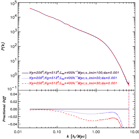
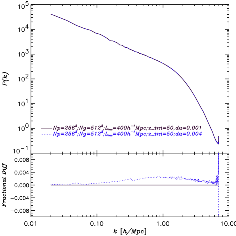
Simulations with lower $z_{\rm ini}$ under estimate the nonlinear power spectrum. Relative to $z_{\rm ini}=100$, $z_{\rm ini}=50$ and $z_{\rm ini}=30$ have power deficits of $1.5\%$ and $3\%$ respectively. These are in good agreement with the results from Crocce et al. (2006). For most of our applications, we use the ratio of the power spectrum. Percent level power deficit is not a concern for us. So we choose $z_{\rm ini}=50$ as our standard initial redshift unless stated otherwise. As to the step size, figure 2 shows that, with $z_{\rm ini}=50$, the power spectrum at $z=0$ differs by less than $0.3\%$ between $da=0.004$ and 0.001. Choosing $da=0.004$ as our standard step size, a full standard run takes anywhere between 10 hours and a day.

Figure 2: Effect of the step size of the simulation on the matter power spectrum at $z=0$. The initial redshift $z_{\rm ini}=50$ and the stepsizes $da$ are listed in the legend. The Nyquist frequency is $k_{\rm Ny}=4\,h{\rm Mpc}^{-1}$. All of our simulations use $da=0.004$ unless stated otherwise.

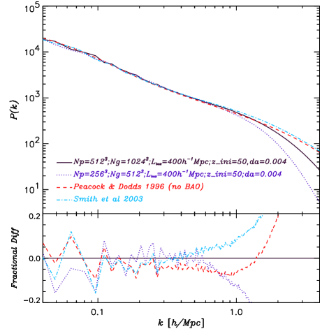
The box size of the simulation is more determined by the $k$ range that a particular application requires than anything else. The Nyquist frequency $k_{\rm Ny}\equiv N^{1/3}_{g}\pi/L_{\rm box}$ is the highest mode that is resolved by the simulation. The lowest mode is $2\pi/L_{\rm box}$. Because of aliasing, not all the $k$ modes in this range are faithfully calculated. To determine the precision of the power spectrum, we use these from simulations with higher resolution ($N_{\rm p}=512^{3}$ and $N_{\rm g}=1024^{3}$) with which we compare the results from our standard simulation ($N_{\rm p}=256^{3}$ and $N_{\rm g}=512^{3}$). With $L_{\rm box}=400h^{-1}{\rm Mpc}$, figure 3 shows that our standard run agrees with the higher resolution run perfectly for $k<0.6h{\rm Mpc}^{-1}$ and the agreement worsens to about $10\%$ at $k=1.0h{\rm Mpc}^{-1}$.

Figure 3: Comparison of the matter power spectrum, at $z=0$, from the simulation with these from fitting formulas of Smith et al. (2003) and Peacock & Dodds (1996). The upper panel shows the matter power spectra $P(k)$ and the lower panel shows the fractional difference of $P(k)$ between the higher resolution simulation with $N_{\rm p}=512^{3}$ and the rest. The simulation box is 400 $h^{-1}{\rm Mpc}$ and the corresponding Nyquist frequencies are $k_{\rm Ny}=4$ and $8\,h{\rm Mpc}^{-1}$ for simulations with $N_{\rm p}=256^{3}$ and $N_{\rm p}=512^{3}$ respectively. The initial power spectrum without BAO peaks is used for the Peacock & Dodds fitting formula.

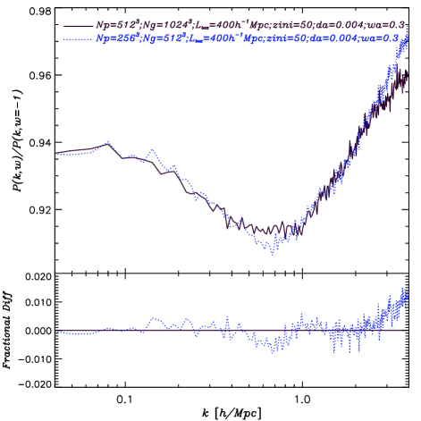
For all of our applications, except for the test of the shifting of peaks in the power spectrum, we use the ratio of power spectra instead of the absolute power. This practice takes care of the sample variance. Figure 4 shows the uncertainty levels of the ratio. Again, we compare our standard run with the one that has higher resolution ($N_{\rm p}=512^{3}$ and $N_{\rm g}=1024^{3}$). For each simulation setup, we run two cosmological models and take the ratio of their power spectra. One cosmological model is $\Lambda$CDM ($w_{0}\equiv w(z=0)=-1$ and $w_{a}\equiv-{{dw}/{da}}|_{a=1}=0$) and the other is $w_{0}=-1$ and $w_{a}=0.3$ model. According to figure 4, the ratios of the power spectra in simulations of different resolutions agree to better than $0.5\%$ all the way to $k\sim 3\,h{\rm Mpc}^{-1}$.

Figure 4: The ratio of the matter power spectra of $w_{a}=0.3$ model to that of $\Lambda$CDM model at $z=0$. Different curves are from simulations with different resolutions which are labeled in the legend. The Nyquist frequencies are $k_{\rm Ny}=4$ and $8\,h{\rm Mpc}^{-1}$ for simulations with $N_{\rm p}=256^{3}$ and $N_{\rm p}=512^{3}$ respectively.

3 the Fate of a Peak in the Initial Power Spectrum

3.1 Setting up the experiment

To address the issue of whether nonlinear evolution of the power spectrum would shift the position of BAO peaks, we construct the following numerical experiment. We put an artificial sharp peak in the otherwise smooth initial matter power spectrum and evolve it using a PM simulation (Shandarin & Melott (1990); Bagla & Padmanabhan (1997) used similar setups to test the transfer of power among different scales). The initial peak is located at $k\sim 0.2h{\rm Mpc}^{-1}$ with a $FWHM=0.013h{\rm Mpc}^{-1}$ and the maximum at $k=0.2051h{\rm Mpc}^{-1}$. At the maximum, $P(k)$ is ten times what it would be without the peak. The location of the peak is at about where the third peak of the BAO sits and deep in the nonlinear regime today. The reason to use a sharp peak is to make it easier to detect peak shifting without using any sophisticated analysis. To set the peak amplitude high is to overcome the sample variance of the simulation which is at least at the level of the BAO peaks ($10\%$). Techniques have been developed to get around sample variance and make BAO features easily seen in simulations. For example, the Millennium Simulation group (Springel et al., 2005) corrects the power spectrum of the actual realization of the initial fluctuations in their simulation to the expected input power and apply these scaling factors at all other times. It is not clear that these scaling factors are not affected by nonlinear evolution. To test the physics behind it, our approach is much cleaner.

The requirement for the simulation is such that $k=0.2h{\rm Mpc}^{-1}$ is well resolved and the peak is sampled with at least a few points in $k$ space. With these considerations, we use a simulation with box size of $2h^{-1}{\rm Gpc}$, number of particles $N_{\rm p}=512^{3}$ and number of grid cells $N_{\rm g}=1024^{3}$. The corresponding Nyquist frequency is $1.6h{\rm Mpc}^{-1}$ and the peak is in the well resolved scale. With this simulation setup, the peak is sampled with five points in $k$ space.

3.2 The shifting of the peak

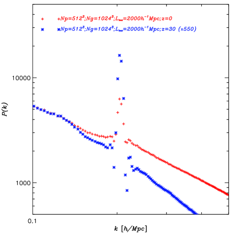
Figure 5 shows the position of the peak at $z=30$ and $z=0$. Table 1 lists the positions $k$ and the corresponding $P(k)$ for the points within the peak.

Figure 5: Testing the shift of peaks in the initial power spectrum. The blue asterisks show the linear power spectrum at $z=0$. The nonlinear power spectrum at $z=0$ is shown using red plus signs. While the peak is being smeared by nonlinear evolution, the position of the peak is not shifted at all.

Table 1: Peak position and height.

	2nd left	1st left	the peak	1st right	2nd right
$k$	0.198	0.201	0.204	0.207	0.211
$P(k;z=30)$	5.442	17.75	29.66	26.11	11.53
$P(k;z=0)$	2884.	4664.	6265.	5616.	3632.
Smearing	0.96	0.48	0.38	0.39	0.57
iVolume	48870	51554	54090	54314	56910

The most conservative estimate of how much does the peak shift is to assume that at $z=0$ the maximum of the peak is somewhere between the second left ($k=0.198\,h{\rm Mpc}^{-1}$) and second right ($k=0.211\,h{\rm Mpc}^{-1}$) points relative to the highest point of the peak in figure 5. We also know that the maximum of the input peak is at $k=0.204\,h{\rm Mpc}^{-1}$; So if the peak has shifted, the shift is less than $(0.211-0.204)/0.204=3.2\%$.

One reasonable assumption we can make is that there is only one peak. This narrows down the maximum to somewhere between the first left ($k=0.201\,h{\rm Mpc}^{-1}$) and first right ($k=0.207\,h{\rm Mpc}^{-1}$) points. With the input maximum known, the shift of the peak is less than $1.6\%$.

We can certainly do better than these crude estimates. One simple method we use is to fit the power spectrum local to the peak with a power law plus a Gaussian. The fits for the power spectra at $z=0$ and $z=30$ are shown in figure 7 and figure 6. The centers of the peak are found to be at $0.205092\,h{\rm Mpc}^{-1}$ and $0.205133\,h{\rm Mpc}^{-1}$ respectively. They agree to $0.02\%$. This estimation is approaching the theoretical limit and for any practical purpose this is equivalent to no shift.

Figure 6: Fitting the $z=30$ power spectrum near the peak with a power law plus a Gaussian. The peak position $k_{\rm peak}$ and width $\sigma_{k}$ are labeled in the legend.

Figure 7: Fitting the $z=0$ power spectrum near the peak with a power law plus a Gaussian. The peak position $k_{\rm peak}$ and width $\sigma_{k}$ are labeled in the legend.

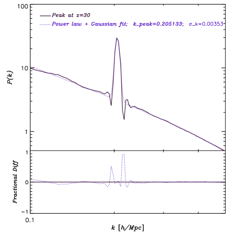
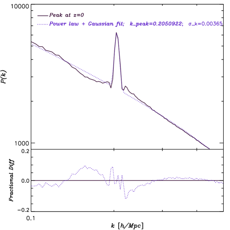
These simple arguments have not taken errors into account. Sample variance does not apply here because the initial peak and the final peak is from the same realization. The Poisson errors are on the level of $0.4\%$. This is too small to change the ordering of the points in the peak, so the first two estimations are not affected. The last estimation would have an uncertainty of $\sim 10^{-6}$ which is too small to be relevant.

3.3 Other effects that could shift the BAO peaks

There are effects other than nonlinear collapse could shift the BAO peaks. The experiment above is dark matter simulation, but the actual tracer of BAO peaks are galaxies which we know is biased tracer of dark matter. If galaxy bias is scale dependent, it could potentially shift the peaks. As shown in White (2005), and Smith et al. (2006), this is indeed the case and the scale dependency should be carefully calibrated.

Another worry is that BAO peaks sit on top of the smooth underline power spectrum whose slope changes due to nonlinear evolution might shift the peaks. As pointed out in Eisenstein, Seo, & White (2006) that this need not be the case. The argument is that one can easily make a template of the smooth underline power spectrum against which to achieve an unbiased measurement.

3.4 Effects of the peak on nonlinear power spectrum

To see the effects of the peak on nonlinear power spectrum, we compare the nonlinear power spectra evolved from initial power spectra with and without artificial peak. The smooth part of these initial power spectra are set to have the same amplitude. Note that this is different from requiring the same $\sigma_{8}$ which would allocate more power to the no peak case on scales outside the peak which would certainly make things more complicated and less clean. The simulation we use for this test is with $N_{\rm p}=256^{3}$, $N_{\rm g}=512^{3}$, $L_{\rm box}=400h^{-1}{\rm Mpc}$ and the corresponding Nyquist frequency is $k_{\rm Ny}=4h{\rm Mpc}^{-1}$. We start the simulation at $z=30$ and the step size is $da=0.004$. The higher Nyquist frequency is the main reason that we use this run instead of the one used for the peak position test.

The result is shown in figure 8.

Figure 8: Comparison of power spectra in simulations with or without a peak in the initial power spectrum. The comparison is done at a few redshifts to show the evolution of the peak and the nonlinear power spectrum. It is clear that Peacock & Dodds (1996) like mapping between linear and nonlinear $k$ does not exist. Instead, the effect of the peak is close to what halo model would predict.

Figure 9: Comparison of power spectra predicted by halo model for the cases with or without a peak in the linear power spectrum. The comparison is done at $z=0$. The effect of the peak on the nonlinear power spectrum is similar to that from simulation (figure 8), but different in details.

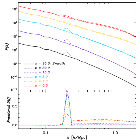
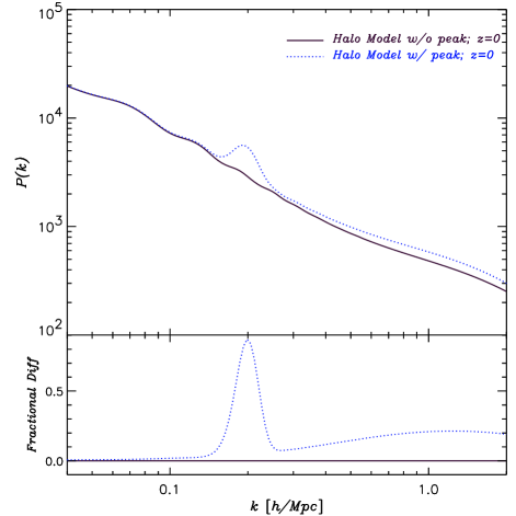
We see that the peak is washed out as the system evolves and the nonlinear power is boosted at all scales smaller than the scale where the peak is located. The amount of boost in power shows no scale dependency.

The mapping between linear and nonlinear scale proposed by Hamilton et al. (1991) and adopted by Peacock & Dodds (1996) would have predicted that the peak being mapped to a nonlinear scale $k_{NL}$ which increases as the nonlinear power grows. We do not see that kind of mapping here. On the other hand, the result is similar to what halo model’s approach would predict. In the halo model, the one halo term (see equation 6) is determined by the halo profile and the halo mass function $n(m)$. The halo profile has nothing to do with whether there is a peak in the matter power spectrum or not. An extra peak in the linear power spectrum would increase the halo mass function below certain mass threshold determined by the position of the peak. As a result, the nonlinear power are boosted on small scales which is close to what we observe in this test. In detail, it does not agree with halo model’s prediction perfectly. As shown in figure 9, halo model predicts that the fractional boost in power due to the existence of a peak has some weak scale dependence which is slightly different from what we see in the simulation. Since the addition of a spike in the power spectrum only changes the mass function at the low mass end where $u(k|m)$ is scale independent at $k=$ a few tenths $h{\rm Mpc}^{-1}$, the one halo term acts like a shot noise term. The fractional difference of the power spectra is scale dependent due to the addition of this short noise like term to the power spectrum. We do not yet understand what accounts for this difference between halo model and the simulation.

4 Linear Growth Function and non-linear Matter Power Spectrum

Existing fitting formulas of matter power spectrum, Peacock & Dodds (1996), Smith et al. (2003) or a simple Halo model, have the following assumption: the nonlinear power spectrum does not depend on the time evolution (history) of the linear power spectrum; it is determined by the linear power spectrum at the same epoch.

There is a weaker version of the assumption, which states that the linear power spectrum plus its time evolution determine the nonlinear power spectrum. A halo model incorporating merger history is a good example of building fitting formula of nonlinear matter power spectrum under this weaker assumption.

In this section, we test both versions of the above assumption using carefully chosen dark energy models.

4.1 Dark energy models construction

We choose the set of binned growth suppression $G_{i}\equiv D_{+}(a_{i})/a_{i}$ and equation of state of dark energy $w_{i}$ as parameters to be considered. $G_{i}$ and $w_{i}$ share the same binning with $\Delta z=0.1$. The linear response of $G_{i}$ to the perturbations of $w_{i}$ can be described by,

$$\delta G_{i}=R_{ij}\delta w_{j}\,.$$ (20)

Operationally the perturbation in $w_{i}$ is achieved by modulating the amplitude of the form,

$$S_{w}\propto\exp\left[-{(z-z_{i})^{\alpha}\over{2\sigma_{z}^{2}}}\right]\,,$$ (21)

where $\alpha=8$ is used to make the shapelet sharp, and $\sigma_{z}=0.05$ is used ($2\sigma_{z}=0.1$ is the binning size). The resulting $w_{i}$ binnings are slightly overlapping which does not affect the applications considered in this work. $G_{i}$ is simply chosen as the growth suppression at the center of the redshift bin $z_{i}$. The response matrix $R_{ij}$ is calculated numerically using the formula in Hu & Eisenstein (1999).

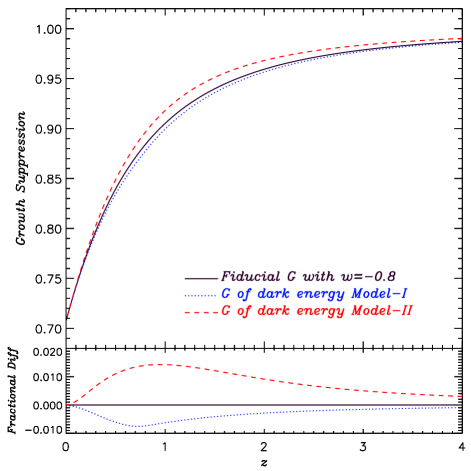
To test the strong assumption, we want to construct a $w$ model that leads to the same growth factor as the $w=w_{\rm const}$ model at $z=0$ but different growth in the past. In order to keep the linear growth factor at $z=0$ the same, the $w$ model we are looking for should have an equation of state greater than $w_{\rm const}$ during some epochs and smaller during some other epochs (to offset the effect on linear growth when it is greater). So we choose $w_{\rm const}=-0.8$, instead of -1, to avoid having $w_{i}<-1$. There are many ways to achieve our goal. The response matrix $R_{ij}$ is invertible. So one could either specify the linear growth and derive the corresponding $w_{i}$ or the other way around. Here we use the latter. First we know that the $w$ model being sought after satisfies the constrain $\delta G_{1}=0=R_{1j}\delta w_{j}$, where we explicitly label the redshift bin at $z=0$ as bin number 1. Furthermore, we restrict the variation of $w$ to below redshift one where the effect of dark energy dominates. Finally we demand that $w(z)>-1$. We then assign values to $\delta w_{j}$ satisfying the above conditions. One of our choices of $w_{i}$ is shown in figure 10 (model-I). Figure 11 shows the comparison of the corresponding linear growth suppression to that of $w=-0.8$ model. Our construction is successful since the two dark energy models have the same linear growth at $z=0$ and a maximum deviation from each other by $0.8\%$ at $z\sim 0.7$.

Figure 10: The time evolution of the equation of state of dark energy. Model-I & II have the same linear growth functions at $z=0$ as that of $w=-0.8$ model but different in the past. Their growth function comparisons are shown in figure 11. Model-III has the same linear growth function (precise to $0.05\%$ as shown in figure 13), at all redshift, as that of $w=-0.8$ model.

Figure 11: Comparison of the growth function of $w=-0.8$ model with these of the constructed dark energy model-I & II which are shown in figure 10. These dark energy models have the same growth functions at $z=0$, but different time evolutions. The fractional differences shown in the lower panel are relative to $w=-0.8$ model.

Figure 12: Comparison of the matter power spectrum at $z=0$ of $w=-0.8$ model with these of the constructed dark energy model-I & II which are shown in figure 10. These dark energy models have the same growth functions at $z=0$ but different time evolutions. The fractional differences shown in the lower panel are relative to $w=-0.8$ model. The simulation box size is $L_{\rm box}=100h{\rm Mpc}^{-1}$ and the Nyquist frequency is $k_{\rm Ny}=16h{\rm Mpc}^{-1}$ .

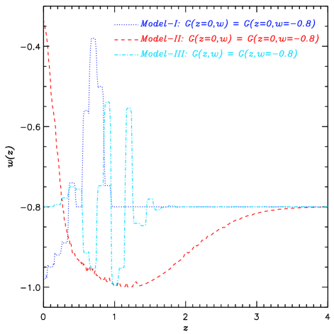
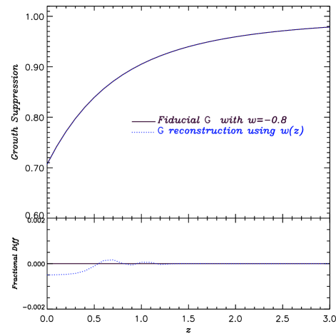
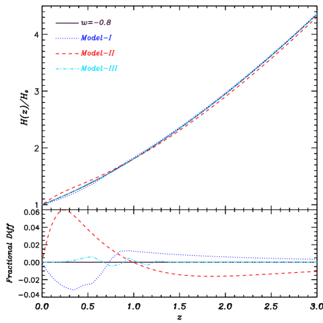
To test the weaker version of the assumption, we want to construct a $w$ model that predicts the same (to certain precision) linear growth function as that of $w=-0.8$ model at all redshift. We apply singular value decomposition (SVD) to the response matrix $R_{ij}$ and select the eigenvectors that have small eigenvalues. These eigenvectors correspond to the combinations of $\delta w_{i}$ to which $\delta G_{i}$ has the least response. Among the selected modes we pick the ones that involve variations of $w_{i}$ at low redshift where the effect of dark energy dominates. Only one mode passed the selection criteria and is shown in figure 10 as model-III. The linear growth of the selected $w$ model agrees with that of $w=-0.8$ model better than $0.05\%$ at all redshift as shown in figure 13. On the other hand, the expansion histories of these two models differ by $\sim 0.6\%$ as shown in figure 14.

Figure 13: Comparison of the growth function of $w=-0.8$ model with that of a wiggling $w(z)$ model-III which is shown in figure 10. The linear growth functions of these two dark energy models agree to better than $0.05\%$ at all redshift.

Figure 14: Comparison of the expansion history $H(z)/H_{0}$ of $w=-0.8$ model with dark energy models whose equations of state are shown in figure 10.

Figure 15: Comparison of the matter power spectrum at $z=0$ of $w=-0.8$ model with that of dark energy model-III which is shown in figure 10. The linear growth functions of these two dark energy models agree to better than $0.05\%$ at all redshift. We conclude that the two $P(k)$ are consistent.

4.2 History does matter

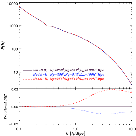
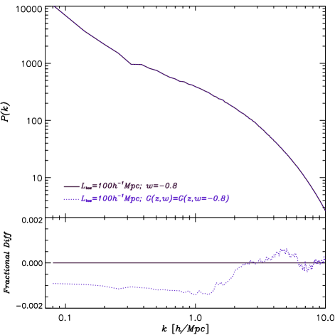
Figure 12 and 15 summarize the results. As shown in figure 12, the nonlinear matter power spectra at $z=0$ are different between $w=-0.8$ model and the constructed dark energy model-I (figure 10) which has the same linear growth at $z=0$ but different during the past. So the nonlinear power spectrum does care about the time evolution of the linear power spectrum, contrary to what existing fitting formulas assume. Our interpretation is the following. The difference in the linear power spectrum during the past causes some differences in the nonlinear power spectrum which would stay there unless some rather delicate adjustments of the history of the linear power spectrum is done to offset the effect. An arbitrary history of the linear power spectrum does not have the ability to undo the difference in the nonlinear power spectrum. One possibility is that different linear growth histories would produce different halo merger histories on which the halo concentration depends (Weshsler et al., 2005). So the nonlinear power spectrum which mainly comes from the one halo term would be different. It is hard to imagine that simply matching the linear growth at $z=0$ would erase the difference. So in general the difference would be there as shown in our test case.

The effect of linear growth history on nonlinear power spectrum is by no means limited to the $\sim 0.8\%$ level shown in our test case. The nonsmooth nature of $w(z)$ also would not make our argument any weaker. By a little bit of more work, we come up with another example that has much smoother $w(z)$ curve (figure 10 model-II) and matching linear growth at $z=0$ but maximum difference of $\sim 1.5\%$ in the past (figure 11 dash line). As shown in figure 12 (dash line), the resulting nonlinear power spectra have maximum difference at $\sim 2\%$ level. From these examples, we see that the difference of the nonlinear power spectrum due to different linear growth history is at the level of the maximum deviation of the corresponding linear power spectra in the past.

Our test of the weaker assumption validates it as shown in figure 15. The nonlinear power spectra of $w=-0.8$ model and the constructed dark energy model-III (figure 10) are consistent with being essentially the same given the small difference of the linear power spectra. This is not a proof that the history of the linear power spectrum fully determines the nonlinear power spectrum, but it hints that it is possibly the case. Note that although there is basically no hope of distinguishing the two apparently very different dark energy models using their growth functions, their expansion histories differ by $\sim 0.6\%$ (see figure 14) which is close to the level that BAO could potentially have some handle on.

5 Matter Power Spectrum and the Equation of State of Dark Energy

With the ambitious observational efforts focused on measuring the equation of state of dark energy to high precision (DES,SNAP,LSST,PanSTARRS), theoretical parameter forecasts will need to be done more carefully than before. In particular, we have to have a better understanding of the nonlinear power spectrum which is very important for cosmic shear and any other probes that utilize the information of growth of density perturbations. Since numerical simulations are too expensive to run for every application, fitting formulas of the matter power spectrum are widely used. The ones provided by Peacock & Dodds (1996) and Smith et al. (2003) are calibrated using $\Lambda$CDM models. McDonald et al. (2005) provided a correction factor to the above mentioned fitting formulas for cosmology with constant $w$ (see also Ma et al., 1999). For two parameter dark energy models parameterized by $w_{0}$ and $w_{a}$, Linder & White (2005) gives a simple procedure to calculate the nonlinear matter power spectrum with a few percent accuracy. While the method provided by Linder & White (2005) has not yet been widely adopted, a common practice is to apply Peacock & Dodds (1996) and Smith et al. (2003) fitting formulas regardless of the dark energy models. In this work we evaluate how well this common practice works.

Two things could go wrong if we used an inaccurate fitting formula. One is that the fitting formula predicts the wrong amplitude of the matter power spectrum. This is the part we study in this work. Another effect of incorrect fitting formula is that the predicted model parameter degeneracy directions and/or extent of the directions are off. Although not covered in this study, the latter effect is very important when the parameters are highly degenerate. During our study of the effect of photo-z on weak lensing tomography (Ma et al., 2006), we noticed that with no tomography binning the extent of the degeneracy among dark energy parameters could differ by a factor of 4 depending on whether the fitting forms of Peacock & Dodds (1996) or halo model is used to calculate the matter power spectrum.

For this study we further restrict ourself to two parameter dark energy models which are parametrized by $w_{0}$ and $w_{a}$.

5.1 The findings

The quantity we use to evaluate the performance of the fitting formulas applied to $w_{a}\neq 0$ dark energy models is,

$$Q\equiv{P(k,w)\over{P(k,w=-1)}}-1,$$ (22)

which is the fractional difference of the matter power spectrum between $w_{a}$ model, $P(k,w)$, and the $\Lambda$CDM model, ${P(k,w=-1)}$. The fractional difference of the power spectrum in terms of $Q$ is $\Delta Q/(Q+1)$ and that of the derivative of the power spectrum is $\Delta Q/Q\equiv Q(fitting\,\,formula)/Q(simulation)-1$. Figures 16-18 show the comparison of this quantify $Q$ from the simulation with those from the fitting formulas of Peacock & Dodds (1996) and Smith et al. (2003) for $w_{a}=0.3$, $0.2$ and $0.1$ respectively.

Figure 16: Performance of the fitting formulas when applied to non-$\Lambda$CDM cosmology. In this particular case, $w_{0}=-1.0$ and $w_{a}=0.3$. The simulation box is 400 $h^{-1}{\rm Mpc}$ and the corresponding Nyquist frequency is $k_{\rm Ny}=4\,h{\rm Mpc}^{-1}$. The initial power spectrum without BAO peaks is used for the Peacock & Dodds fitting formula.

Figure 17: Performance of the fitting formulas when applied to non-$\Lambda$CDM cosmology. In this particular case, $w_{0}=-1.0$ and $w_{a}=0.2$. The simulation box is 400 $h^{-1}{\rm Mpc}$ and the corresponding Nyquist frequency is $k_{\rm Ny}=4\,h{\rm Mpc}^{-1}$. The initial power spectrum without BAO peaks is used for the Peacock & Dodds fitting formula.

Figure 18: Performance of the fitting formulas when applied to non-$\Lambda$CDM cosmology. In this particular case, $w_{0}=-1.0$ and $w_{a}=0.1$. The simulation box is 400 $h^{-1}{\rm Mpc}$ and the corresponding Nyquist frequency is $k_{\rm Ny}=4\,h{\rm Mpc}^{-1}$. The initial power spectrum without BAO peaks is used for the Peacock & Dodds fitting formula.

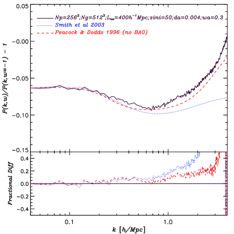
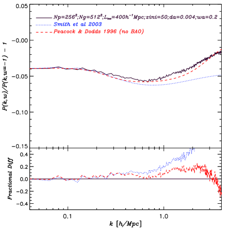
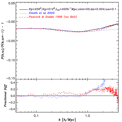
First of all, the fitting formulas are doing a good job describing $w_{a}$ models. The fractional difference of the power spectrum is $\Delta Q/(Q+1)\sim 1\%$ and that of the derivative is $\Delta Q/Q\sim 10\%$ for $k<1.0\,h{\rm Mpc}^{-1}$. In the context of Fisher matrix analysis, the Fisher matrix elements would be $20\%$ off at most. Again, just to remind ourself that we are only considering the effect of the amplitude of the power spectrum but not that of the shape of the power spectrum which is closely tied to the degeneracy direction of the model parameters.

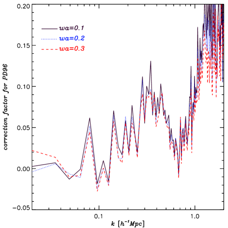
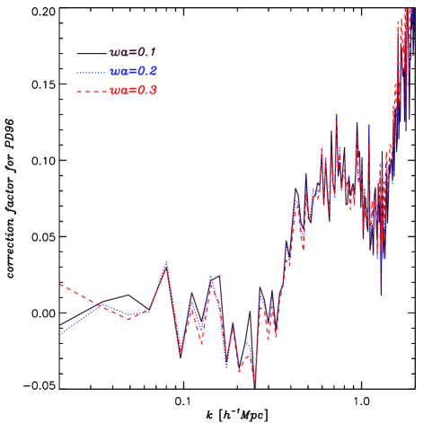
The most surprising result we find is that the fractional differences in $Q$ from Peacock & Dodds (1996) fitting formula are independent of $w_{a}$, as shown in figure 19. To turn this fact into a fitting formula of the matter power spectrum for $w_{a}$ models, the time evolution of this potential correction factor to Peacock & Dodds (1996) fitting formula should also be independent of $w_{a}$. Figure 20 shows this correction factor at $z=0.62$. We see that the peak of the correction shifts to smaller scale (higher $k$) as one goes to higher redshift and, amazingly, it shows no dependency on $w_{a}$. Although such regular behavior seems always have a good reason behind it, at the moment, we do not have a physical explanation.

Figure 19: The fractional differences of $Q$ (defined in equation 22), $Q(fitting\,\,formula)/Q(simulation)-1$, for different $w_{a}$. The power spectrum is evaluated at $z=0$.

Figure 20: The fractional differences of $Q$ (defined in equation 22), $Q(fitting\,\,formula)/Q(simulation)-1$, for different $w_{a}$. The power spectrum is evaluated at $z=0.62$.

It is very tempting to use such a fact to come up with a correction factor to the fitting formula of Peacock & Dodds (1996). The hump at the nonlinear scale in figure 19 and the ones at high redshift can be fit very well using a Gaussian in $k$ space. However, as we have pointed out throughout this work, the physical arguments supporting Peacock & Dodds’ fitting formula do not seem to hold: the linear and nonlinear scale mapping does not hold; the assumption that the history of the linear growth does not affect the nonlinear power spectrum is also being shown to be incorrect. Adding more corrections to Peacock & Dodds’ fitting formula would only turn it into another ”theory of epicycles”. We do not think this is the right approach to build a good fitting formula. As a short term solution, this may be worth doing. We leave the readers to make the judgment.

6 Discussion and Conclusions

We modify the public PM code developed by Anatoly Klypin and Jon Holtzman to simulate cosmologies with arbitrary initial matter power spectra and the equation of state of dark energy. Using N-body simulation, we test various aspects of the matter power spectrum, including whether nonlinear evolution would shift the BAO peaks, the assumptions that go into constructing fitting formulas of the nonlinear power spectrum, and the precision of the existing fitting formulas when applied to dark energy models parametrized by $w_{0}$ and $w_{a}$.

Any shift of the BAO peaks in the matter power spectrum would bias the cosmological distance inferred hence the cosmological parameters derived. To test whether nonlinear evolution would shift BAO peaks, we implement an artificial sharp peak in the initial power spectrum and evolve it using the PM code. We find that the position of the peak is not shifted by nonlinear evolution. An upper limit of the shift at the level of $0.02\%$ is achieved by fitting the power spectrum local to the peak using a power law plus a Gaussian. This implies that, for any practical purpose, the baryon acoustic oscillation peaks in the matter power spectrum are not shifted by nonlinear evolution. There are other effects such as galaxy bias that could potentially shift the peaks. These should be carefully calibrated as well.

We also find that the existence of a peak in the linear power spectrum would boost the nonlinear power at all scales evenly. This is contrary to what HKLM scaling relation predicts, but roughly consistent with that of halo model. The scale dependence is slightly different from halo model prediction in detail. Further study is required to understand the cause of the difference.

All existing fitting formulas of the nonlinear power spectrum assume that the linear power spectrum uniquely determines the nonlinear one, regardless of the linear growth history. To test this assumption, we construct two dark energy models with the same linear power spectra today but different linear growth histories and compare their nonlinear power spectra from the simulation. We find that the resulting nonlinear power spectra differ at the level of the maximum deviation of the corresponding linear power spectra in the past. Similarly, two constructed dark energy models with the same growth histories result in consistent nonlinear power spectra. This is consistent with but not a proof of the conventional wisdom that together, the linear power spectrum and the linear growth history uniquely determine the nonlinear power spectrum.

Next generation large-scale structure surveys need better fitting formulas than what are available now. With the high accuracy required, new fitting formulas should be based on solid foundations. Our results suggest that we should abandon HKLM scaling relation, keep halo model and further include linear growth history to build the next generation fitting formulas of nonlinear power spectrum. Note that our study only includes dark matter. To build fitting formulas with percent level accuracy, one has to include the effect of baryons (White, 2004; Zhan & Knox, 2004; Jing et al., 2006) and substructure (Hagan et al., 2005).

For simple dark energy models parametrized by $w_{0}$ and $w_{a}$, the existing nonlinear power spectrum fitting formulas, which are calibrated for $\Lambda$CDM model, work reasonably well. The corrections needed are at percent level for the power spectrum and $10\%$ level for the derivative of the power spectrum. We find surprisingly that, for Peacock & Dodds (1996) fitting formula, the corrections needed to the derivative of the power spectrum are independent of $w_{a}$ but changing with redshift. As a short term solution, a fitting form could be developed for $w_{0}$, $w_{a}$ models based on this fact.

References

- Abazajian et al. (2005) Abazajian, K., Zheng, Z., & Zehavi, I. et al, 2005, ApJ, 625, 613
- Aldering et al. (2004) Aldering, G. et al. 2004, PASP, submitted (astro-ph/0405232)
- Amendola et al. (2005) Amendola, L., Quercellini, C., & Giallongo, E., 2005, MNRAS, 357, 429
- Bagla & Padmanabhan (1997) Bagla, J.S., & Padmanabhan T., 1997, MNRAS 286, 1023
- Blake & Bridle (2005) Blake, C., & Bridle, S., 2005, MNRAS, 363, 1329
- Blake & Glazebrook (2003) Blake, C., & Glazebrook, K., 2003, ApJ, 594, 665
- Cole et al. (2005) Cole, S., et al., 2005, MNRAS, 362, 505
- Cooray, Hu, Huterer & Joffre (2001) Cooray, A., Hu, W., Huterer, D., & Joffre, M., 2001, ApJ, 557, L7
- Crocce et al. (2006) Crocce, M., Pueblas, S., & Scoccimarro, R., 2006, astro-ph/0606505
- Dolney et al. (2006) Dolney, A., Jain, B., & Takada, M., 2006, MNRAS, 366, 844
- Eisenstein et al. (2005) Eisenstein, D., Zehavi, I., Hogg, D. et al, 2005, ApJ. 633, 560-574
- Eisenstein, Hu, & Tegmark (1998) Eisenstein, D., Hu, W., & Tegmark, M., 1998, ApJ, 504, L57
- Eisenstein et al. (2006) Eisenstein, D., Seo H., Sirko, E., & Spergel D., 2006, astro-ph/0604362
- Eisenstein, Seo, & White (2006) Eisenstein, D., Seo H., & White M., 2006, astro-ph/0604361
- Fosalba, Gaztanaga, & Castander (2003) Fosalba, P., Gaztanaga, E., & Castander, F., 2003, ApJ 597, L89-92
- Glazebrook & Blake (2005) Glazebrook, K., & Blake, C., 2005, ApJ, 631, 1
- Hamilton et al. (1991) Hamilton, A. J. S., Kumar, P., Lu, E, & Matthews, A., 1991, ApJ, 374, L1-L4
- Hagan et al. (2005) Hagan, B., Ma, C., & Kravtsov, A., 2005, ApJ, 633, 537
- Hu & Eisenstein (1999) Hu, W., & Eisenstein, D., 1999, Phys. Rev. D. 59, 083509 (astro-ph/9809368)
- Huff et al. (2006) Huff, E., Schulz, A.E., White, M., Schlegel, D.J., Warren, M.S., 2006, astro-ph/0607061
- Hu & Haiman (2003) Hu, W., & Haiman, Z., 2003, Phys. Rev. D, 68, 063004
- Huterer & Takada (2005) Huterer, D., & Takada, M., 2005, Astropart. Phys. 23, 369-376 (astro-ph/0412142).
- Jain, Mo, & White (1995) Jain, B., Mo, H.J., & White, S.D.M., 1995, MNRAS, 276, L25-29
- Jarvis, Jain, Bernstein, & Dolney (2005) Jarvis, M., Jain, B., Bernstein, G., & Dolney, D., 2005, astro-ph/0502243
- Jenkins et al. (2001) Jenkins, A., Frenk, C.S., White, S.D.M., Colberg, J.M., & Cole, S. et al., 2001, MNRAS, 321, 372
- Jing et al. (2006) Jing, Y.P., Zhang, P., Lin, W.P., Gao, L., & Springel, V., 2006, ApJ, 640, L119-122
- Linder (2003) Linder, E. V., 2003, Phys. Rev. D, 68, 063504
- Linder (2005) Linder, E., 2005, astro-ph/0507308
- Linder & White (2005) Linder, E., & White, M., 2005, Phys. Rev. D 72, 061304 (astro-ph/0507308).
- Ma et al. (1999) Ma, C., Caldwell, R. R., Bode, P., & Wang, L. 1999, ApJ, 521, L1
- Matsubara (2004) Matsubara, T., Szalay, A. S., & Pope, A. C., 2004, ApJ, 606, 1
- Ma et al. (2006) Ma, Z., Hu, W., & Huterer, D., 2006, ApJ, 636, 21-29 (astro-ph/0506614).
- McDonald et al. (2005) McDonald, P., Trac, H. and Contaldi, C., 2005, astro-ph/0505565
- Navarro, Frenk, & White (1997) Navarro, J.F., Frenk, C.S., & White, S.D.M., 1997, ApJ, 490, 493
- Peacock & Dodds (1994) Peacock, J., & Dodds, S., 1994, MNRAS, 267, 1020-1034
- Peacock & Dodds (1996) Peacock, J., & Dodds, S., 1996, MNRAS, 280, L19
- Peebles (1980) Peebles, P.J.E., The Large-Scale Struncture of the Universe, 1980, p266
- Peebles & Yu (1970) Peebles, P. J. E., & Yu, J. T., 1970, ApJ,162, 815
- Press & Schechter (1974) Press, W., & Schechter, P., 1974, ApJ, 187, 425
- Scranton et al. (2003) Scranton, R., Connolly, A., Nichol, R. et al., 2003, astro-ph/0307335
- Seljak et al. (2005) Seljak, U. et al., 2005, Phys. Rev. D, 71 103515
- Seljak et al. (2003) Seljak, U., Sugiyama, N., White, M., & Zaldarriaga, M., 2003, Phys. Rev. D68, 83507
- Seo & Eisenstein (2003) Seo, H., & Eisenstein, D., 2003, ApJ, 598, 720
- Shandarin & Melott (1990) Shandarin, S., & Melott, A., 1990, ApJ, 364, 396
- Sheth & Cooray (2002) Sheth, R.K., & Cooray, A., 2002, Phys. Rev., 372, 1
- Sheth & Tormen (1999) Sheth, R.K., & Tormen, B., MNRAS, 1999, 308, 119
- Smith et al. (2003) Smith, R., Peacock, J., Jenkins, A. et al., 2003, MNRAS 341, 1311-1332
- Smith et al. (2006) Smith, R., Scoccimarro, R., Sheth, R., 2006, astro-ph/0609547
- Spergel et al. (2003) Spergel, D.N. et al., 2003, ApJS, 148, 175
- Springel et al. (2005) Springel, V., White, S., Jenkins, A, et al. 2005, Nature, 435, 629-636 (astro-ph/0504097)
- Sunyaev & Zel’dovich (1970) Sunyaev, R. A., & Zel’dovich, Ya. B., 1970, Ap&SS, 7, 3
- Tegmark et al. (2004) Tegmark, M. et al., 2004, Phys. Rev. D, 69, 103501
- Weshsler et al. (2005) Weshsler, R., Zentner, A., Bullock, J., Kravtsov, A., & Allgood, B., 2005, ApJ in press, astro-ph/0512416
- White (2004) White, M., 2004, Astropart. Phys., 22, 211-217
- White (2005) White, M., 2005, astro-ph/0507307
- Zel’dovich (1970) Zel’dovich, Y. B., Astron. Astrophys., 1970, 5, 84-89
- Zhan & Knox (2004) Zhan, H., & Knox, L., 2004, ApJ, 616, L75-78