Information content in the halo-model dark-matter power spectrum II: Multiple cosmological parameters

Abstract

We investigate the cosmological Fisher information in the non-linear dark-matter power spectrum in the context of the halo model. We find that there is a plateau in information content on translinear scales which is generic to all cosmological parameters we tried. There is a rise in information on smaller scales, but we find that it is quite degenerate among different cosmological parameters (except, perhaps, the tilt). This suggests that it could be difficult to constrain cosmological parameters using the non-linear regime of the dark-matter power spectrum. We suggest ways to get around this problem, such as removing the largest haloes from consideration in survey analysis.

1 Introduction

The distribution of matter in the Universe on large scales contains a wealth of cosmological information. Even though galaxy redshift surveys provide a huge amount of data about galaxy clustering on non-linear scales, it is unclear how useful these smaller scales are cosmologically. Using $N$-body simulations, Rimes & Hamilton (2005, RH05; 2006, RH06) investigated the amount of cosmological information, as a function of scale, in the matter power spectrum $P(k)$. They found that information about $\ln A$, the initial amplitude of the linear power spectrum, is preserved in $P(k)$ on large, linear scales, and that there is significant information on small scales, but there is little independent information on translinear scales ($k\sim 0.2-0.8{\ }h^{-1}{\,}{\rm Mpc}$). Neyrinck, Szapudi & Rimes (2006, Paper I) found that the halo model also predicts this translinear plateau in the information about $\ln A$ in $P(k)$. Paper I showed that the translinear plateau came largely from cosmic variance in the number of the largest haloes in a given volume.

In this Letter, we extend the analysis of Paper I, looking at how well $P(k)$ can constrain multiple cosmological parameters simultaneously.

2 Method

The Fisher information matrix $F_{\alpha\beta}$ about parameters $\alpha$ and $\beta$ given a set of data is defined (Fisher, 1935; Tegmark, Taylor & Heavens, 1997) as the concavity of the natural logarithm of the likelihood function $\mathcal{L}$, averaged over an ensemble of data predicted by $\mathcal{L}$;

$$F_{\alpha\beta}\equiv-\left\langle\frac{\partial^{2}\ln\mathcal{L}({\rm data}|\alpha,\beta,{\rm priors})}{\partial\alpha\,\partial\beta}\right\rangle.$$ (1)

In this Letter, we investigate the (hereafter, implicitly non-linear, dark-matter) power spectrum $P_{i}=P(k_{i})$ (actually, $\ln P_{i}$), measured in bins of wavenumber $k_{i}$. The cumulative Fisher information over a range of bin indices $i\in\mathcal{R}$ is

$$F_{\alpha\beta}(\mathcal{R})=\sum_{i,j\in\mathcal{R}}-\left\langle\frac{\partial\ln P_{i}}{\partial\alpha}\frac{\partial^{2}\ln\mathcal{L}}{\partial\ln P_{i}\partial\ln P_{j}}\frac{\partial\ln P_{j}}{\partial\beta}\right\rangle.$$ (2)

To simplify this, we approximate the expectation value of the data Fisher matrix as $\textbf{{C}}^{-1}$, the inverse of the data covariance matrix $C_{ij}\equiv\left\langle\Delta\ln P_{i}\Delta\ln P_{j}\right\rangle$. This approximation is good if estimates of $\ln P_{i}$ have Gaussian distributions about their expectation values. This seems to be adequately so for measurements of the dark-matter power spectrum (RH06), as the central limit theorem would encourage one to think. We denote the data covariance matrix as C (with Fisher matrix $\textbf{{C}}^{-1}$), and denote the parameter Fisher matrix as F (with covariance matrix $\textbf{{F}}^{-1}$). Equation (2) becomes

$$F_{\alpha\beta}(\mathcal{R})=\sum_{i,j\in\mathcal{R}}\frac{\partial\ln P_{i}}{\partial\alpha}(\textbf{{C}}_{\mathcal{R}}^{-1})_{ij}\frac{\partial\ln P_{j}}{\partial\beta},$$ (3)

where $\textbf{{C}}_{\mathcal{R}}$ is the square submatrix of C with both indices ranging over $\mathcal{R}$.

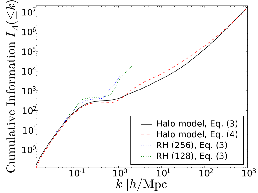
The definition in Eqn. (3) is equivalent to the one used in RH06, except that it bypasses the step of explicit upper-Cholesky decorrelation. However, Eqn. (3) differs from the erroneous definition used in RH05 and Paper I, for which derivative terms were used only on the diagonal. This previous definition can be written

$$F_{\alpha\beta}^{\rm old}(\leq k_{\rm max}) = \sum_{k_{i}\leq k_{\rm max}}\frac{\partial\ln P_{i}}{\partial\alpha}\frac{\partial\ln P_{i}}{\partial\beta}\times$$ (4)

$$\left[\sum_{l,m\leq i}(\textbf{{C}}_{\leq i}^{-1})_{lm}-\sum_{l,m\leq i-1}(\textbf{{C}}_{\leq i-1}^{-1})_{lm}\right],$$

where $\textbf{{C}}_{\leq i}$ is the upper-left square submatrix of C with indices only through $i$. Figure 1 shows the difference this makes in the cumulative information in $\ln A$, using the same cosmology as in Paper I. The difference is small, but could be larger for a parameter with derivative terms farther from unity than $\ln A$. We also show the measurements from simulations (RH06), calculated using Eqn. (3).

Figure 1: Different definitions of cumulative information, $F_{\ln A,\,\ln A}(\leq k)$, about $\ln A$ in the dark-matter power spectrum ($I_{A}(\leq k)$ is the notation used in Paper I.) The red, dashed curve uses the incorrect, ‘old’ information definition, used in Paper I and RH05, while the black curve uses the correct definition, used in this Letter, and RH06. The dotted curves show what RH06 found from $N$-body simulations of box size 128 and 256${\ }h^{-1}{\,}{\rm Mpc}$, using the ‘new’ definition.

2.1 Covariance matrix construction

We use the same procedure for the matter power spectrum covariance matrix as in Paper I. The covariance of the power spectrum in a survey of volume $V$ is the sum of a Gaussian term, which depends on the square of the power spectrum itself, and a term involving the (hereafter, implicitly non-linear) trispectrum (Hamilton, Rimes & Scoccimarro, 2006; Scoccimarro, Zaldarriaga & Hui, 1999, SZH);

$$C_{ij}=\frac{1}{V}\left[\frac{(2\pi)^{3}}{V_{s,i}}2P(k_{i})^{2}\delta_{ij}+T_{ij}\right],$$ (5)

where $V_{s,i}$ is the volume of shell $i$ in Fourier space (proportional to $k_{i}^{3}$ for logarithmically spaced bins), and $T_{ij}$ is the trispectrum averaged over shells $i$ and $j$;

$$T_{ij}\equiv\int_{s,i}\int_{s,j}T({\mn@boldsymbol{k}}_{i},-{\mn@boldsymbol{k}}_{i},{\mn@boldsymbol{k}}_{j},-{\mn@boldsymbol{k}}_{j})\frac{d^{3}{\mn@boldsymbol{k}}_{i}}{V_{s,i}}\frac{d^{3}{\mn@boldsymbol{k}}_{j}}{V_{s,j}}.$$ (6)

We use the halo-model formalism (Cooray & Sheth, 2002) to get the non-linear matter power spectrum and trispectrum. In the halo model, the universe is assumed to consist of virialized haloes distributed according to leading-order perturbation theory (the first-order, linear, power spectrum, the second-order bispectrum, and the third-order trispectrum). In the halo model, the power spectrum is the sum of one- and two-halo terms, and the trispectrum is the sum of one-, two-, three-, and four-halo terms (Cooray, 2001; Cooray & Hu, 2001, CH). For example, the power spectrum is

$$P(k) = P^{\rm 1h}(k)+P^{\rm 2h}(k)$$ (7)

$$= M^{0}_{2}(k,k)+P^{\rm lin}(k)[M^{1}_{1}(k)]^{2},$$ (8)

where $M^{\beta}_{\mu}$ are integrals over the halo mass function;

$$M^{\beta}_{\mu}(k_{1},\ldots,k_{\mu}) \equiv \int\int\left(\frac{m}{\bar{\rho}}\right)^{\mu}b_{\beta}(m)n(m,c)$$ (9)

$$\times u(k_{1},m,c)\cdots u(k_{\mu},m,c)\,dc\,dm.$$

Here, $\bar{\rho}$ is the mean matter density, $m$ is the halo mass, $c$ is the halo concentration in the NFW profile (Navarro, Frenk & White, 1996), $b_{\beta}(m)$ is the $\beta$-order halo bias (Mo, Jing & White, 1997; Scoccimarro et al., 2001), and $u(k,m,c)$ is the halo profile in Fourier space, normalized to unity at $k=0$. In Eqn. (8), we assume that the power spectrum $P^{\rm hh}$ of a set of haloes is a uniformly biased linear power spectrum $P^{\rm lin}$, even though this seems not to be quite true (Smith, Scoccimarro & Sheth, 2006, SSS).

For the covariance matrix, we use use the same halo-model inputs as did CH, except that we use a Sheth & Tormen (1999) halo mass function. The baseline cosmology is a flat concordance model, specifically that found recently by the WMAP team (Spergel et al., 2006), except that $n=1$, i.e. $(\Omega_{m}h^{2}=0.127,\,\Omega_{b}h^{2}=0.0223,\,n=1,\,\sigma_{8}=0.74)$. For the input linear power spectrum, we use the camb code.

2.2 Parameter derivatives

Figure 2: Parameter derivatives $\partial\ln P(k)/\partial\alpha$ (where $\alpha$ is the parameter shown on the left), computed using two methods: our halo model code (black curves) and the Smith et al. (2003) fitting function (green curves). Where the curves are dashed, the derivatives are negative. The red dotted $\partial\ln P(k)/\partial\ln A$ curve was measured from 400 $N$-body simulations by RH05.

The other major ingredients in our analysis are the derivatives of $\ln P_{i}$ with respect to parameters of interest. In Paper I, we varied $\ln A$ by small amounts, and thus calculated $\partial\ln P_{i}/\partial\ln A$ numerically. In this Letter, we do the same with the parameters $(\ln A,\,n,\,\ln h,\,\ln f_{b},\,\ln\Omega_{m}h^{2})$. Here, $A$ and $n$ are the scalar amplitude and tilt of the power spectrum, using the default camb pivot point, at $0.05\,{\rm Mpc}^{-1}$. The parametrized Hubble constant $h=H_{0}/(100\,\rm{km\ sec^{-1}\ Mpc^{-1}})$, and $f_{b}$ is the baryon fraction $\Omega_{b}/\Omega_{m}$, where $\Omega_{b}$ is the baryon density, and $\Omega_{m}$ is the sum of $\Omega_{b}$ and the dark-matter density, $\Omega_{c}$. We assume a flat Universe throughout.

We tried two different methods to calculate the parameter derivatives: using our halo model code; and, using the halofit  (implemented in camb) fitting formula developed by Smith et al. (2003). Each method has its advantages: using our code would be self-consistent, but halofit  has been extensively tested against $N$-body simulations. We expected the results to be similar, though, since halofit  was developed in the spirit of halo models, having both quasi-linear and self-halo terms.

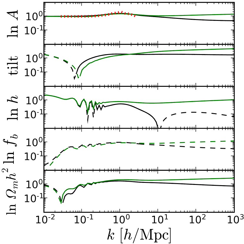
Figure 2 is a comparison of the derivative terms from the two methods. While they give similar results on linear scales, there are qualitative differences on non-linear scales. In general, halofit  predicts greater derivative terms than our code. We also show $\partial\ln P(k)/\partial\ln A$ as measured from 400 128-particle PM $N$-body simulations of box size $256{\ }h{\,}{\rm Mpc}^{-1}$ run by RH05 (using a slightly different cosmology). Although both methods are roughly consistent with the simulation measurement, the continued decrease on smaller scales which occurs in our code is somewhat more plausible than the upturn seen with halofit. The methods differ most dramatically for $\ln h$; our halo model code predicts a tiny variation with $\ln h$ on small scales, while halofit  predicts a variation comparable to other cosmological parameters.

The two models give different predictions on small scales because of different ways the one-halo terms $P^{1\rm h}$ (dominant on small scales) are defined. In the halo model, $P^{1\rm h}$ depends only on the abundances and concentrations of haloes of different masses; these depend on the variance in the linear density field smoothed with a top-hat filter of radius $r$, $\sigma^{2}(r)$. Keeping all of our other parameters fixed, changing $h$ merely shifts $\ln P^{\rm lin}(k)$ horizontally and vertically. For this cosmological model, the shift is such that $P^{\rm lin}(k)$ does not change if the local slope ${\rm d}\ln P^{\rm lin}(k)/{\rm d}\ln k$ reaches a value $\approx-2$. This happens at small scales, so $\sigma^{2}(r)$ does not change appreciably for small $r$. Thus, the abundance and concentration of small haloes varies only slightly with $\ln h$, and $P^{1\rm h}$ hardly changes on small scales. On the other hand, the halofit power spectrum does vary with $\ln h$ on small scales, since it explicitly depends on $\Omega_{m}$. (In both cases, we hold $\Omega_{m}h^{2}$ constant.)

3 Results

The parameter Fisher matrix $F_{\alpha\beta}$ gives predictions of statistical error bars and error ellipsoids, assuming that the likelihood functions are Gaussian. This assumption does not precisely hold, but is adequate to look for trends. Holding all other parameters fixed, the variance in a parameter $\alpha$ is $1/F_{\alpha\alpha}$, while the variance marginalized over other parameters is $(\textbf{{F}}^{-1})_{\alpha\alpha}$, where F is the Fisher matrix including $\alpha$ and the other parameters.

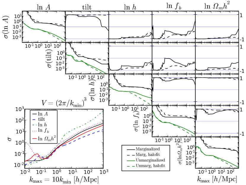
Figure 3a shows how constraints on our chosen parameters change with the smallest scale (largest wavenumber) used in the analysis. We use a survey volume of $256{\ }h^{-1}{\,}{\rm Mpc}$, and a fixed lowest wavenumber, $0.02{\ }h{\,}{\rm Mpc}^{-1}$ $\approx 2\pi/(256{\ }h^{-1}{\,}{\rm Mpc})$. In Fig. 3, instead of the rather abstract quantity of information, we show probably more familiar error-bar half-widths.

Figure 3: (A, Upper-right). One-sigma error-bar half-widths on various cosmological parameters as a function of the highest wavelength considered, $k_{\rm max}$. The lowest wavelength is held constant at 0.02${\ }h{\,}{\rm Mpc}^{-1}$, and a volume of $(256{\ }h^{-1}{\,}{\rm Mpc})^{3}$ is used. Plots on the diagonal show error-bar half-widths in single parameters, both unmarginalized (black) and marginalized over all four other parameters (green). For the solid curves, we use our halo model code for parameter derivatives; for the dashed, we use halofit. Off-diagonal plots show correlation coefficients between pairs of parameters, in the marginalized covariance matrix $\textbf{{F}}^{-1}$. (B, Lower-left). A crude exploration of practical issues of survey size. We show unmarginalized one-sigma error-bar half-widths in various cosmological parameters, holding the dynamic range of scales used constant, at a factor of 10, and using parameter derivatives from our halo model code. The volume of the box changes with $k_{\rm max}=10k_{\rm min}$; we imagine measuring the power spectrum in a box of volume $(2\pi/k_{\rm min})^{3}$.

Diagonal plots show error-bar half-widths, both unmarginalized, $1/\sqrt{F_{\alpha\alpha}}$ (black), and marginalized over all four other parameters, $\sqrt{(\textbf{{F}}^{-1})_{\alpha\alpha}}$ (green). The solid and dashed curves use the halo-model and halofit  derivative terms, respectively. For example, the information about $\ln A$ as plotted in Fig. 1 appears (to the $-1/2$ power) in the solid black curve in the upper-left plot.

Off-diagonal plots show correlation coefficients $R_{\alpha\beta}\equiv(\textbf{{F}}^{-1})_{\alpha\beta}/\sqrt{(\textbf{{F}}^{-1})_{\alpha\alpha}(\textbf{{F}}^{-1})_{\beta\beta}}$, in the marginalized parameter covariance matrix $\textbf{{F}}^{-1}$ containing all five parameters. If $R_{\alpha\beta}\approx\pm 1$, then an error ellipse is squashed along a diagonal line; if $R_{\alpha\beta}=0$, then the ellipse is circular.

The main conclusions of this Letter come from Fig. 3a. The cumulative information in a parameter varied alone generally has the characteristics found in RH05 and Paper I: there is a plateau on translinear scales, followed by a rise on fully non-linear scales. This rise appears as a drop in Fig. 3a, which shows the information to the power $-1/2$. Unfortunately, this small-scale error-bar tightening is quite degenerate among parameters. The green curves on the diagonal display this clearly; with the possible exception of the tilt, marginalized error-bar half-widths level off in the translinear regime, and never significantly decrease as smaller scales are included in the analysis. This degeneracy is also visible in the correlation coefficients, many of which are nearly $\pm 1$ on small scales. Small scales provide an increased lever arm for constraining the tilt on small scales, but the marginalized error bars in the tilt only tighten significantly if using our code’s derivative terms, not those from halofit.

Why is the small-scale rise in information so degenerate among parameters? As discussed above, $P^{\rm 1h}$ is entirely determined by the abundances and concentrations of haloes, which depend on integrals (over top-hat window functions) of the linear power spectrum. Altering any single parameter will indeed change these integrals, but this change will generally be close to a monolithic shift up or down in $P^{\rm 1h}$. Thus, changing any parameter will have a similar effect on the small-scale power spectrum.

Our previous plots have shown the cumulative information up to a wavenumber $k_{\rm max}$, holding $k_{\rm min}$ and the volume fixed. In Fig. 3b, we crudely explore the effects of survey size. We show unmarginalized error-bar half-widths, computed using derivatives from our code (not halofit), changing the volume of the survey, but not the range of scales measured. For a box size $b$, we assume that $P(k)$ can be measured from $k_{\rm min}=2\pi/b$ to $k_{\rm max}=10k_{\rm min}$. Here, the translinear plateau takes the form of a steep ramp upward at $k_{\rm max}\approx 1{\ }h{\,}{\rm Mpc}^{-1}$.

3.1 Looking in rural areas of the Universe

In Paper I, we argued that the translinear information plateau in $P(k)$ is caused by cosmic variance in the number of the largest haloes in a given volume, since on translinear scales, large haloes dominate $P(k)$. A potential way around this problem is to model the contribution of the largest haloes to the power spectrum. Another way could be to remove the ‘noise’ of the largest haloes from the analysis. Even beyond the cosmic-variance argument, it is plausible that cosmological information is especially obscured in large haloes, in advanced stages of non-linear collapse. This is not a new idea; for example, much cosmological information seems to lie in the low-overdensity Lyman-alpha forest (e.g. Croft et al., 2002; Gnedin & Hamilton, 2002).

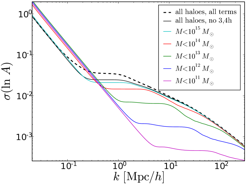
To investigate the potential of cutting out large haloes from the analysis, we truncate the halo-model integrals over the halo mass function at various upper mass cut-offs. For this calculation, we use only the dominant 1h and 2h terms in the trispectrum; we explain why in the rest of the paragraph. In this Letter, we assume that the $P^{\rm hh}$ and $T^{\rm hh}$ are given by leading-order-perturbation-theory (LOPT). This is not quite the case (SSS), but more accurate estimates of $P^{\rm hh}$ and $T^{\rm hh}$ are not currently known. The LOPT power spectrum $P^{\rm lin}$ is first-order, but the LOPT trispectrum $T^{\mathcal{O}(3)}$ is third-order; as SZH point out, using both of them together is inconsistent. Indeed, we find that doing so in Eq. 5 gives off-diagonal entries exceeding unity in the correlation matrix, violating the Schwarz inequality. These unruly entries are in the translinear regime, where $T^{\mathcal{O}(3)}$ may still accurately trace the non-linear trispectrum, but $P^{\rm lin}$ does not trace the non-linear power spectrum. Using the full halo mass spectrum in the halo model, this inaccuracy does not matter substantially, since where $P^{\rm lin}$ and $T^{\mathcal{O}(3)}$ may not accurately trace $P^{\rm hh}$ and $T^{\rm hh}$ (in the non-linear regime), the terms in the trispectrum which involve them are buried under other terms. So, we use all terms in the halo-model trispectrum when using the full halo mass function. On the other hand, if large haloes are missing from the mass spectrum, the raw $P^{\rm hh}$ and $T^{\rm hh}$ are exposed on translinear scales, and the inconsistency of using $P^{\rm lin}$ and $T^{\mathcal{O}(3)}$ together matters. One way to keep the order of perturbation theory consistent would be to calculate all functions to third order, a laborious task that might not give a more accurate result. Instead, we assume, as before, that $P^{\rm hh}=P^{\rm lin}$, but exclude terms involving functions of higher than first order in the halo-model trispectrum (the 3h and 4h terms).

Figure 4 shows that cutting out the largest haloes from the mass function for all quantities indeed shifts the information plateau to smaller scales, giving tighter error bars. We also show the results if all terms are included in the trispectrum and no mass cut-off is made; this shows that the 1h and 2h terms do dominate the halo-model trispectrum in this case.

Figure 4: The effect of introducing a mass cut-off in the halo mass function on error-bar half-widths on $\ln A$. Again, $V=(256{\ }h{\,}{\rm Mpc}^{-1})^{3}$. The information in the power spectrum of matter in low-mass haloes is potentially greater than in the full matter distribution. For the solid curves, only the dominant one- and two-halo terms of the halo-model trispectrum are included; for the dashed curve, the full trispectrum is used, including the three- and four-halo terms.

There are many practical problems which would make it difficult to constrain cosmological parameters by removing large haloes from the analysis. Halo masses are difficult to measure, and measuring all halo masses in a survey seems nearly impossible. But perhaps something as simple as the number of galaxies in a halo is well-enough correlated with halo mass to make a dent in the translinear plateau. Other problems could include inadequate knowledge of halo power spectra on non-linear scales, and the effects on a survey mask from excising haloes. Still, the information gains with mass cut-offs are dramatic enough that it seems to be worth exploring how to get around these issues.

4 Conclusion

In the context of the halo model, we find that the matter power spectrum is rather disappointing for cosmological parameter estimation on scales smaller than linear. On translinear scales ($k\sim 1-10{\ }h{\,}{\rm Mpc}^{-1}$), there is a high degree of intrinsic (co)variance in the matter power spectrum caused by cosmic-variance fluctuations in the number of large haloes, which suppress the information in any parameter of current interest on those scales. There is information on even smaller scales if each parameter is varied alone, but we find that this information is quite degenerate among various cosmological parameters. This is because changing any parameter affects the small-scale matter power spectrum in a similar way, close to a uniform shift up or down in the one-halo term. There could be more independent information in the tilt on small scales, but one method we used (involving halofit) to calculate the non-linear power spectrum predicts that the information in the tilt is also somewhat degenerate.

Our results suggest that useful cosmological information is scant below linear scales in the full matter power spectrum, but this is probably not the case for all large-scale structure statistics. For example, we show that in the halo model, the power spectrum of matter outside of large haloes has an information plateau on smaller scales than does the full matter power spectrum, allowing tighter constraints on cosmological parameters. There are practical problems with this specific approach, but it raises hopes that there are ways to circumvent the covariance and degeneracies among cosmological parameters which haloes introduce on non-linear scales. In addition, the smallest scales of the galaxy power spectrum contain information about galaxy formation. Despite the apparent difficulties we have found, we remain confident that worthwhile information exists on non-linear scales in the spatial distribution of certain sets of galaxies, matter, or even haloes themselves.

References

- Cooray (2001) Cooray A., 2001, PhD thesis, Univ. Chicago
- Cooray & Hu (2001) Cooray A., Hu W., 2001, ApJ, 554, 56 (CH)
- Cooray & Sheth (2002) Cooray A., Sheth R., 2002, Phys. Rep., 372, 1
- Croft et al. (2002) Croft R.A.C., Weinberg D.H., Pettini, M., Hernquist, L., Katz, N., 2002, ApJ, 520, 1
- Fisher (1935) Fisher R.A., 1935, J.Roy.Stat.Soc., 98, 39
- Gnedin & Hamilton (2002) Gnedin, N.Y., Hamilton, A.J.S., 2002, MNRAS, 334, 107
- Hamilton, Rimes & Scoccimarro (2006) Hamilton A.J.S., Rimes C.D., Scoccimarro R., 2006, MNRAS, 371, 1188
- Mo, Jing & White (1997) Mo, H.J., Jing, Y.P., White, S.D.M., 1997, MNRAS, 284, 189
- Navarro, Frenk & White (1996) Navarro J., Frenk C., White S.D.M., 1996, ApJ, 462, 563
- Neyrinck, Szapudi & Rimes (2006) Neyrinck, M.C., Szapudi, I., Rimes C.D., 2006, MNRAS, 370, L66 (Paper I)
- Rimes & Hamilton (2005) Rimes C.D., Hamilton A.J.S., 2005, MNRAS, 360, L82 (RH05)
- Rimes & Hamilton (2006) Rimes C.D., Hamilton A.J.S., 2006, MNRAS, 371, 1205 (RH06)
- Scoccimarro, Zaldarriaga & Hui (1999) Scoccimarro R., Zaldarriaga M., Hui L., 1999, ApJ, 527, 1 (SZH)
- Scoccimarro et al. (2001) Scoccimarro R., Sheth R., Hui L., Jain B., 2001, ApJ, 546, 20
- Sheth & Tormen (1999) Sheth R.K., Tormen G., 1999, MNRAS, 308, 119
- Smith, Scoccimarro & Sheth (2006) Smith R.E., Scoccimarro R., Sheth R.K., 2006, MNRAS, submitted (astro-ph/0609547)
- Smith et al. (2003) Smith R.E. et al., 2003, MNRAS, 341, 1311
- Spergel et al. (2006) Spergel D.N., et al., 2006, ApJ, submitted (astro-ph/0603449)
- Tegmark, Taylor & Heavens (1997) Tegmark M., Taylor A.N., Heavens A.F., 1997, ApJ, 480, 22