The UKIRT Infrared Deep Sky Survey First Data Release

Abstract

The First Data Release (DR1) of the UKIRT Infrared Deep Sky Survey (UKIDSS) took place on 2006 July 21. UKIDSS is a set of five large near–infrared surveys, covering a complementary range of areas, depths, and Galactic latitudes. DR1 is the first large release of survey-quality data from UKIDSS and includes 320 deg² of multicolour data to (Vega) $K=18$, complete (depending on the survey) in three to five bands from the set ZYJHK, together with 4 deg² of deep JK data to an average depth $K=21$. In addition the release includes a similar quantity of data with incomplete filter coverage. In JHK, in regions of low extinction, the photometric uniformity of the calibration is better than 0.02 mag. in each band. The accuracy of the calibration in ZY remains to be quantified, and the same is true of JHK in regions of high extinction. The median image FWHM across the dataset is $0.82\arcsec$. We describe changes since the Early Data Release in the implementation, pipeline and calibration, quality control, and archive procedures. We provide maps of the areas surveyed, and summarise the contents of each of the five surveys in terms of filters, areas, and depths. DR1 marks completion of 7 per cent of the UKIDSS 7-year goals.

1 Introduction

UKIDSS is the UKIRT Infrared Deep Sky Survey (Lawrence et al., 2006), carried out using the Wide Field Camera (WFCAM; Casali et al., 2006) installed on the United Kingdom Infrared Telescope (UKIRT). Data acquisition for the survey started in 2005 May. A prototype dataset, the Early Data Release (EDR), was released on 2006 February 10, and is described in Dye et al. (2006) (hereafter D06). The present paper defines the UKIDSS First Data Release (DR1), the first large release of UKIDSS survey-quality data. The data were released to the ESO community on 2006 July 21, and are available from http://surveys.roe.ac.uk/wsa.

UKIDSS is a programme of five imaging surveys that each uses some or all of the broadband filter complement $ZYJHK$, and that span a range of areas, depths, and Galactic latitudes. There are three high Galactic latitude surveys, providing complementary combinations of area and depth; the Large Area Survey (LAS), will cover 4000 deg² to $K=18$, the Deep ExtraGalactic Survey (DXS), 35 deg² to $K=21$, and the Ultra Deep Survey (UDS), 0.8 deg² to $K=23$. There are two other wide surveys to $K=18$, aimed at targets in the Milky Way; the Galactic Plane Survey (GPS) will cover 1900 deg², and the Galactic Clusters Survey (GCS) 1100 deg². The complete UKIDSS programme is scheduled to take seven years, requiring $\sim$1000 nights on UKIRT. The current implementation strategy is focused on completing an intermediate set of goals, defined by the ‘2-year plan’ detailed in D06. All magnitudes quoted in this paper use the Vega system described by Hewett et al. (2006). Depths, where not explicitly specified, are the total brightness of a point source for which the flux integrated in a $2\arcsec$ diameter aperture is detected at $5\sigma$.

A set of five baseline papers provides the relevant technical background information for the surveys. The overview of the programme is given by Lawrence et al. (2006). This sets out the science goals that drove the design of the survey programme, and details the final coverage that will be achieved, in terms of fields, areas, depths, and filters. The camera is described in detail by Casali et al. (2006), and the ZYJHK photometric system is characterised by Hewett et al. (2006), who provide synthetic colours for a wide range of types of star, galaxy, and quasar. Details of the data pipeline and data archive will appear in Irwin et al. (2007, in prep.) and Hambly et al. (2007, in prep.), respectively.

The EDR (D06), cited earlier, contains a sample of the data obtained in 2005, and amounts to about one per cent of the 7-year plan. The EDR represented a step towards regular release of survey-quality data, and occurred while the quality-control (QC) procedures were still being developed, and the pipeline finalised. The EDR included all data from the first observing block, 05A (2005 April to June), and the DXS and UDS data up to the end of September in block 05B (2005 August to 2006 January). The 05B dataset is substantially larger, and was processed with a later version of the pipeline. The current release, DR1, includes all the 05A and 05B data. All the 05B data have been verified using the revised QC procedures that define ‘survey quality’. The 05A data, however, are included in DR1, almost unchanged from the EDR (the minor changes are detailed in section 3.5) i.e. with the older versions of the pipeline and QC procedures. In a similar manner to the EDR, two databases are provided in this release. The DR1 database includes all data where the full filter complement for a particular survey exists, and the DR1+ database (which is a superset of the DR1 database) includes all data that have passed QC. The next observing block, 06A, 2006 May to July, will be combined with the 05A and 05B data, and released in DR2, early in 2007.

Each UKIDSS data release will be accompanied by a paper summarising the contents of the release, and detailing procedural changes since the previous release. The EDR paper, D06, is a self-contained summary of all information relevant to understanding the contents of the EDR. It serves as the baseline paper for technical details for all releases, and in the current paper only changes in technical details are documented. The terms EDR and DR1 have been copied from the Sloan Digital Sky Survey (SDSS), and the aims of the UKIDSS EDR and DR1 papers are similar to those of the SDSS EDR (Stoughton et al., 2002) and DR1 (Abazajian et al., 2003) papers. Besides providing details of the contents of the EDR database, D06 includes relevant details of the camera design, the observational implementation (integration times, microstepping), the pipeline and calibration, data artifacts, and the quality control procedures, as well as a brief guide to querying the archive.

In the current paper, in Section 2 we illustrate the fields surveyed on an all-sky map. In Section 3 we detail differences in the implementation, pipeline and calibration, quality control, and archive procedures between EDR and DR1. In Section 4 we provide maps for each survey, illustrating the coverage of the DR1 release. In Section 5 we summarise the contents of DR1 in terms of areas and depths, and other relevant quantities.

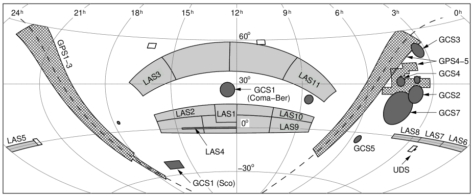
Figure 1: The UKIDSS 2–year plan survey areas showing the LAS (solid light grey), GPS (cross-hatched), GCS (solid dark grey), DXS (empty squares) and UDS (lying alongside the western-most DXS field). The dashed line indicates the Galactic plane. LAS, GPS, GCS projects included in DR1 are marked. The names of the GCS clusters not labeled are Pleiades (GCS2), Alpha Per (GCS3), Tau.–Aur. (GCS4), Orion (GCS5), and Hyades (GCS7).

2 Overview of DR1 fields

In this section we provide an overview of the areas surveyed in DR1. Detailed coverage maps are provided in Section 4. Fig. 1 illustrates the areas that will be covered in the 2-year plan. The LAS areas are shaded light grey, the GPS areas are cross-hatched, and the GCS areas are shaded dark grey. The DXS targets are the four white rectangles with centres as follows; XMM-LSS (2${}^{\rm h}25^{\rm m}$,$-4^{\circ}30^{\prime}$), the Lockman Hole (10${}^{\rm h}57^{\rm m}$,+57${}^{\circ}40^{\prime}$), Elais N1 (16${}^{\rm h}10^{\rm m}$,+54${}^{\circ}00^{\prime}$), and VIMOS 4 (22${}^{\rm h}17^{\rm m}$,+0${}^{\circ}20^{\prime}$). The UDS field covers a single tile, 0.8deg², and is just visible to the W of the DXS XMM-LSS field.

For administrative purposes the surveys are divided into ‘projects’. The LAS, GPS, and GCS projects which contain observations released in DR1 are illustrated in the figure. In the LAS, the data from projects LAS$1-4$ were observed in 05A, and were released in the EDR, and are included in DR1 unchanged, with one proviso. This is that the algorithm for associating detector frames (Section 3.5), in merging sources across bands, has been refined. For some sources, in regions where frames overlap, a different choice of frame has resulted in revised photometry. New projects LAS$5-11$ were observed in 05B. The GPS is divided into two main regions. The eastern wing lies mostly between $18^{\rm h}$ and $23^{\rm h}$ and was observed in 05A, in project GPS1. These data were released in the EDR, and are included here unchanged (with the above proviso). The eastern wing was also observed in 05B, in projects GPS2 and 3. The western wing covers the Galactic plane between approximately $3^{\rm h}$ and $8^{\rm h}$, and an additional region below the plane, the Taurus–Auriga–Perseus molecular cloud complex. The western wing was observed in 05B in projects GPS4 and 5. In the GCS, the targets Sco and Coma–Ber were observed in 05A in project GCS1. These data were released in the EDR, and are included here unchanged. In 05B the following targets were observed: Pleiades, Alpha Per, Tau.–Aur., Orion, and Hyades. Coordinates for the complete list of GCS targets are provided in Table 3 in D06.

In the DXS, the Lockman Hole was observed only in 05A, Elais N1 and XMM-LSS were observed in 05A and 05B, and VIMOS4 was observed only in 05B. The Lockman Hole data, and data taken in Elais N1 and XMM–LSS up to 2005 Sept 27, were released in the EDR. These data are included in DR1, with minor differences. Firstly the QC for the 05B data has been redone, together with the (later) 05B data not included in the EDR, using the revised procedures detailed in Section 3. Secondly, in all fields the stacking has been redone for DR1, having fixed two problems that were evident in the EDR stacking (D06). The UDS was only observed in 05B, and has been treated in the same way i.e. the QC for all the data released in DR1 was done in a homogeneous manner following the revised procedures.

3 Update

D06 contains details of the implementation, pipeline, calibration, quality control, and archive procedures applied to the EDR data, and a glossary of technical terms. In this section we describe the differences between the procedures applied to the 05B data for DR1, and those applied to the 05A data for the EDR.

Scheme	Filter	$t_{\rm exp}$	$\mu$-step	Offsets	$t_{\rm tot}$
(Survey)		(s)			(s)
1 (LAS)	$Y$	20	no	2-pt	40
	$J$	5	$2\times 2$	2-pt	40
	$HK$	10	no	4-pt	40
2 (LAS)	$Y$	20	no	4-pt	80
	$J$	10	$2\times 2$	2-pt	80
	$HK$	10	no	8-pt	80
3 (GCS)	$ZY$	20	no	2-pt	40
	$JH$	10	no	4-pt	40
	$K$	5	$2\times 2$	2-pt	40
4 (GPS)	$JH$	10	$2\times 2$	2-pt	80
	$K$	5	$2\times 2$	2-pt	40
	$H_{2}$	20	$2\times 2$	2-pt	160
5 (DXS)	$JK$	10	$2\times 2$	16-pt	640
6 (UDS)	$JK$	10	$3\times 3$	9-pt	810

Table 1: The implementation schemes used for the five surveys in 05B.

3.1 Implementation

The basic observational unit of the surveys is the stack multiframe, which is the set of four frames (one for each detector) formed by combining the set of exposures, of individual length $t_{\rm exp}$, and combined length $t_{\rm tot}$, at a given base position. The shallow surveys, LAS, GCS, and GPS, are built up by tiling the survey areas with these stack frames. For the deep surveys, DXS, and UDS, deep stack frames are created by averaging several stack frames at each position, and the fields are tiled with these deep stack frames.

The observing strategy incorporates flexibility, in order to make the best use of the observing time allocated. For example, projects suitable for execution in non–photometric conditions are included, as well as when the seeing is mediocre in photometric conditions. Small changes were made to the observing strategy for the 05B block in the light of experience in the 05A block for the LAS, GCS, and DXS. The revised set of implementation schemes for 05B (update of Table 4 in D06) is provided in Table 1. The same scheme has been retained for subsequent observations, to date. For each scheme, the table lists successively a reference number, the filters to which the details apply, the exposure time, the microstepping (if used), the number of offset positions (other than microsteps), and the total integration time $t_{\rm tot}$ making up the stack frame.

The changes since 05A are as follows. For the DXS exposure times were increased from 5s to 10s, to reduce overheads associated with readout. For the GPS the exposure times in $J$ and $H$ were increased from 5s to 10s, to reduce the overheads, and the 4-pt offset pattern replaced by a 2-pt pattern. Observations with the $H_{2}$ filter, used for the first time in 05B, mimic the $JH$ procedure, but with twice the exposure time, 20s, giving a total integration time of 160s. For the LAS and GCS, again in order to reduce overheads, by allowing increased exposure time, microstepping is now only applied in a single filter, $J$ for LAS, and $K$ for GCS. These are the filters where second–epoch observations will be made, for measuring proper motions. The improved sampling provided by microstepping allows more accurate astrometry.

3.2 Pipeline and calibration

3.2.1 Pipeline

The main changes to the pipeline processing since the EDR are a modification of the sky subtraction strategy and the incorporation of an algorithm to reduce the impact of cross-talk images.

The changes to the sky subtraction strategy involved grouping the sky estimation and correction by exposure time within each passband, if possible. This was not necessary for the EDR since virtually all frames in any one passband used identical exposure times. This extra refinement proved necessary due to the presence of a combination of additive and multiplicative artifacts in the sky correction frames. The generally more localised multiplicative artifacts scale closely with exposure time whereas the additive components do not. The latter includes illumination-dependent reset anomaly and pedestal offsets. Because a wide range of observing strategies may be employed over a night, the manner in which to combine data over the night to optimise the sky subtraction is a complex problem. It has proven difficult to devise a general algorithm that does not require manual intervention, and in a few percent of images sky-subtraction residuals are visible. Further improvements to the sky-subtraction algorithm are anticipated.

Cross-talk artifacts are confined within detector quadrants and occur between the eight channels read out in parallel in each quadrant. All the detectors show similar cross-talk patterns with the induced artifacts being essentially time derivatives of saturated stars, with either a ‘doughnut’ appearance from heavily saturated regions or half-moon-like (i.e. positive/negative residual) appearance from only weakly saturated stars. Adjacent cross-talk images are symmetric (with number of channels displacement) and typically induce features at $\sim 1$ per cent of the differential flux of the source in adjacent channels, dropping to $\sim 0.2$ per cent and $\sim 0.05$ per cent in successive channels further out. The size of the effect continues to decline with distance from the source, but in the case of very bright stars in the first or eighth channel, may be detectable out to seven channels distance.

Creating a correction for these artifacts involves devising a robust combination of a model involving the directional time derivative of the primary source, and if possible, comparing and combining this with adjacent cross-talk artifacts to create a correction sub-image. In general this model sub-image is unaffected by the presence of real objects overlapping the artifact and although the time derivative model is only an approximation to the real effect a relatively clean subtraction generally results.

D06 noted two problems affecting stacking of the data in the deep surveys. For the DXS and UDS the basic data product is a leavstack multiframe (i.e. four detectors) of total integration time 640s and 810s respectively (Table 1), referred to here as an intermediate stack. Depth is built up by averaging these intermediate stack frames. The first problem was caused by a safety feature being incorrectly applied, which meant that the recorded value of the sky noise in intermediate stacks was set too high in a few cases. The second problem (which did not affect the UDS) was quantisation noise, due to the use of integer values, affecting the deepest DXS frames. Revised stacking procedures have eliminated both problems.

3.2.2 UDS processing and source detection

The UDS is the only survey which employs $3\times 3$ microstepping. The resulting pixel scale ($0.133\arcsec$) oversamples the typical seeing of the UDS images ($0.7\arcsec$). The image detection algorithm employed in the WFCAM pipeline is optimised for critically sampled, or slightly oversampled, data. As noted in D06, for highly oversampled data, such as for the UDS, the algorithm tends to break up objects into multiple components. Consequently the UDS EDR object catalogues were unsatisfactory in this respect. Because of this, new pipeline procedures have been implemented for the UDS for DR1. The standard WFCAM pipeline is followed, up to creation of the intermediate stack frames. From that point on, further processing, quality control, frame stacking, and catalogue generation have been undertaken by the UDS working group. Full details will be provided in a forthcoming paper (Foucaud et al., 2006). A brief outline of the procedures follows.

All intermediate stacks were visually inspected for defects. In a substantial fraction the sky subtraction was deemed unsatisfactory. This can be imputed to the manner in which data taken at different times in the night were combined to create sky correction frames (Section 3.2.1). The unsatisfactory data were passed through the pipeline again, manually tailoring the sky subtraction process, and the majority of the data were recovered. A further approximately 5 per cent of frames were discarded due to the presence of moon ghosts (see Section 3.3 below). Channel bias offsets (D06) were identified in a few per cent of the frames and were corrected for with a custom procedure. In total 76 per cent of the UDS intermediate stacks were used in the DR1 release.

Before the final stacking, noisy border regions were trimmed from each frame using a masking procedure. Masking was also applied to minor image defects (e.g. satellite trails). The stacking was performed using the Terapix SWARP image resampling tool (Bertin et al., 2002), with flux scaling computed from the calibration zero-points. Images were weighted in the final stack by the inverse variance of the sky. Experimentation confirmed that this improved the final depths by approximately 0.1 mag. The pipeline confidence maps were then used to provide inter-pixel weighting.

Source catalogues were produced using the SExtractor software (Bertin & Arnouts, 2002). The K-band image was used as the primary detection image, since this is deeper than J for most galaxy colours. Simulations were used to optimise the source extraction parameters, as described in detail in Foucaud et al. (2006).

3.2.3 Calibration

The calibration scheme applied for DR1 is exactly the same as used for the EDR (D06): the zero point for each detector in each stack multiframe is determined by identifying suitable 2MASS stars in the frame, and converting the 2MASS magnitudes to the WFCAM ZYJHK system using linear colour equations, listed in D06. The calibration goal is an accuracy of the zero point of 0.02mag. While there are sufficient 2MASS stars on each detector to achieve a precision better than 0.02mag, systematic errors can enter in a variety of ways. We anticipate three changes to the way in which the calibration is undertaken for DR2.

• For stars cooler than spectral type K, typically the colour relations become non-linear, and differences between dwarfs and giants become significant. Therefore in DR2 colour equations will be determined, and applied, over a limited colour range, confined to hotter stars, F to K.

• The colour terms for the Z and Y bands are large, and it has become apparent that these relations are non linear, with a break near the boundary between A and F spectral types. Therefore a colour relation determined from a linear fit to the F to K sequence will result in a constant zero point error. Preliminary analysis indicates that the offset required is larger in the Y band than in the Z band, and is approximately 0.09mag, in the sense that Y magnitudes in the EDR and DR1 should be increased by this amount to place them on the Vega system. Following a more detailed analysis, the DR2 photometry will be corrected for this source of error.

• There is evidence of zero-point errors in regions of high extinction. This is simply a consequence of the fact that the colour relations for extinguished stars will differ from the colour relations for unextinguished stars, and will depend on the extinction. Therefore in highly extinguished regions application of a colour equation determined from regions of low extinction is incorrect.

3.3 Data artifacts

The cause of the bright moon ghosts described by D06 has been traced to the autoguider auxiliary lens that sits at the centre and above the field lens (Casali et al., 2006). When the moon lies within an annulus from about $14^{\circ}$ to $30^{\circ}$ off axis, a ghost is formed by moonlight shining through the auxiliary lens and undergoing a double internal reflection inside the field lens. It is planned to install a baffle tube between the auxiliary lens and the field lens to eliminate these moon ghosts. In the meantime, over the 06A observing block, fields within $30^{\circ}$ of the moon have been avoided. Because the arrays cover only a fraction of the focal plane the moon ghosts also produce scattered light in the instrument, even when no ghost image occurs. Sky subtraction is frequently poor when the moon is within $30^{\circ}$ of the field, although it is not clear whether this is a general problem caused by the moon shining directly on the field lens, or whether it is a consequence of the ghost images, and scattered light within the instrument. Whatever the cause, the majority of images taken in 05A and 05B, when the moon was within $30^{\circ}$, have been deprecated.

3.4 Quality control

The QC procedures followed the same pattern as with the EDR, vis. first removing corrupt data (i.e. meaningless data, e.g. empty array), and bad data (i.e. unusable data, due e.g. to a moon ghost), and then applying a set of QC cuts that define survey quality. The last have now been finalised and we set out the main elements here. The most important parameters defining survey quality are photometric zero point (i.e. how much cloud), average stellar image ellipticity, seeing, and depth. The criteria are detailed below. Some summary statistics quantifying the characteristics of the data are provided in Section 5.

Photometric zero point. Each detector frame is calibrated using the 2MASS photometry of bright unsaturated stars in the frame, using appropriate colour terms. Therefore the computed zero point for each frame, relative to the modal value for that filter, gives an indication of how much extinction by cloud there was. The effect of cloud is to reduce the depth of the observations, but cloud only effects the accuracy of the calibration to the extent that the extinction is variable across the field of view. Therefore, perfectly photometric conditions are not necessarily required for good calibration.

In practice all projects requiring accurate calibration specify ‘photometric’ conditions, and extinction by cloud is monitored during execution. Inevitably, though, a fraction of these observations are undertaken through thin cloud. At the QC stage, for photometric projects we require that the zero point lie within 0.2 mag. of the modal value. In practice the vast majority of observations requesting photometric conditions are undertaken in conditions considerably better than this limit: the root mean square (RMS) variation of the zeropoint for frames specifying photometric conditions is 0.02 mag in JHK.

For some projects photometric conditions are not required, and these are specified as ‘thin cirrus’ at the telescope. These include DXS and UDS observations, since each field is visited repeatedly, and the field may be calibrated if only a single visit takes place in photometric conditions. Additionally ‘repeat’ observations in the shallow surveys (J only in the LAS, K only in the GCS, and K and $H_{2}$ in the GPS) may be undertaken in non–photometric conditions. At the QC stage, for non-photometric projects we require that the zero point lie within 0.3 mag. of the modal value.

Figure 2: Plot of distribution of stellar ellipticity, averaged over each multiframe, within declination slices. Each point marks the median value in all multiframes within the slice, and the error bars denote the 16 per cent to 84 per cent range. Some frames at high declinations suffer from elongated images.

Ellipticity. The mean value of the ellipticity $(e=1-b/a)$ for all the stellar objects in a detector frame is recorded in the archive as the parameter avStellarEll in the table MultiframeDetector. The value of this parameter averaged over the four detectors of a multiframe is used as a QC parameter. In the majority of cases the measured value is less than 0.1, but a proportion of the DR1 frames display elongated images, particularly at high declinations. The extent of the problem is illustrated in Fig. 2 which plots the distribution of the ellipticity parameter over all multiframes observed for DR1 (before any QC deprecations), within slices of declination. The points are the median value, and the error bars mark the 16 per cent to 84 per cent range (equivalent to $\pm 1\sigma$). At high declinations $\delta>40^{\circ}$ there is a pronounced tail towards large values. For projects at high declinations we deprecated multiframes with stellar ellipticity $>0.25$, while a cut $>0.20$ was applied to all other frames.

The cause of the elliptical stellar images has been traced to instrument flexure, as well as uncorrected errors in the primary mirror figure, introducing astigmatism and coma. These problems of image quality were solved in time for 06A observations. Using a model derived from wave-front sensing data, the effects of instrument flexure are now corrected for by tilting and displacing the secondary. Additionally, the telescope temperature and attitude–dependent focus model has been improved for the combined UKIRT/WFCAM system leading to better focus tracking during observing.

Seeing. For the LAS and GCS we required seeing $<1.2\arcsec$ (averaged over the four detectors), except for the single-band non-photometric observations (J in LAS, K in GCS) where the seeing was relaxed to $<1.3\arcsec$. For the GPS, in the plane (i.e. except for observations of Taurus), the requirements were $<1.0\arcsec$ in K, and $<1.1\arcsec$ in J and H. In Taurus the limit was relaxed to $<1.3\arcsec$ in K and H₂, and $<1.4\arcsec$ in J and H. In the DXS the limit was $<1.3\arcsec$, and in the UDS the limit was $<0.8\arcsec$ in K, and $<0.9\arcsec$ in J.

Depth. For the LAS and GCS, detector frames are deprecated if the depth achieved (as defined by D06) is more than 0.5 mag. less deep than the modal value. For the GPS, the depth is affected by confusion noise, and therefore depends on Galactic latitude, $b$. So, for the GPS, depth is plotted against $b$, and outliers are identified and deprecated. There are no specific depth cuts applied to the DXS and UDS observations, since all frames contribute to improving the depth in the deep stack frames. Nevertheless a small number of frames are eliminated that were taken in conditions of bright sky, where the depth is severely compromised.

Visual checks. An additional check is made of each stack frame by viewing the archive jpeg image to identify bad frames not already deprecated by the automated QC procedures. Examples include frames where the sky subtraction is visually unsatisfactory, trailed frames not already identified as such, frames suffering from extreme channel bias offsets (either individual channels or multiple channels), or frames badly affected by bright moon ghosts. Where only a small part of a moon ghost affects the frame, or where the ghost is not particularly bright, the frame may be accepted.

Proportion of frames failing quality control. Summed over all the surveys the proportion of frames that failed QC is close to $20\%$. We expect this figure to fall substantially in future releases, to $<10\%$. The main causes are the following: a.) $7\%$ of frames were duplicated, because the observations were abandoned (principally because the seeing deteriorated), and were later repeated; b.) $8\%$ of frames were rejected because the sky subtraction was unsatisfactory, or bright moon ghosts were present; c.) $4\%$ of frames were rejected because the seeing exceeded the required limits, or the images were elongated.

We expect the proportion in category (a) to be substantially smaller in future releases. If the seeing deteriorates during an observation the observer may abandon the MSB. Unfortunately an earlier version of the summit pipeline failed to keep pace with the observations, when the GPS was observed (because cataloguing the myriad stars was slow), meaning that the QC information was only available after completion of the MSB, so the whole MSB was rejected, when it should have been abandoned earlier. The summit pipeline now keeps up with the observations. Similarly the proportion in category (b) will be smaller, now that the moon ghosts have been eliminated, and with improvements to the sky subtraction algorithm. There should also be some reduction in category (c), with image-quality improvements. Nevertheless failure of a small fraction in this category is considered acceptable, recognising this as a consequence of attempting to use as large a fraction of the observing time as possible, by tailoring the observations to the conditions.

3.5 Archive

Between the EDR and DR1 releases, there have been several minor bug fixes to the archiving software. These are detailed in the release history notes in the online web pages. Some modifications, however, warrant elaboration.

In the EDR, there were a small number of fields where frames were not correctly associated, and this gave rise to incompletely merged sources e.g. the YJHK bands available in LAS fields being merged into two framesets, for example one comprising YJH and the other K only. This in turn led to a small but significant number ($10^{3}$ out of $10^{6}$, or 0.1 per cent) of merged sources of apparently extreme colour when trawling the EDR+ tables for objects appearing in a limited set of the available bands. This bug has been fixed in the DR1 release. At the same time the source merging software (Hambly et al., 2007, in prep.), and the algorithm that associates detector frames into framesets have been refined. As a consequence, for some sources the choice of detector frames making up a frameset has changed between EDR and DR1, and therefore so also has the photometry.

As noted previously, the treatment of both the DXS and UDS in the EDR was suboptimal, mainly in terms of the source extraction applied to each. The code used was the standard nightly pipeline code, and this was not set up to cope with the lower sky noise of the deep surveys (DXS, UDS), or the significant oversampling of the UDS data. For the DXS, a revised procedure of scaling the data numbers before performing source extraction works around the limitations in the software; for the UDS, we have adopted the data yielded by the alternative software and procedures detailed in Foucaud et al. (2006). No changes to the standard archive data model were required by either of these procedural modifications, but the online documentation for the UDS has been substantially altered to correctly describe the changes to the archive web pages.

4 Fields observed in DR1

In this section we provide maps of the areas covered in DR1. In cases where the maps provided in D06 have not required updating, they are not repeated here. This is made clear when describing each survey.

Figure 3: Coverage by LAS 05B observations, showing data coverage in the DR1 database (all of YJHK; dark–grey tiles only), and the DR1+ database (all tiles). Each small square is a detector frame. The physical size of a detector in this plot and in the GCS plot (Fig. 4), is twice as large as in the two GPS plots (Figs 5 and 6).

4.1 Large Area Survey

In 05A the projects observed were LAS1, 2, 3, 4. The maps for these projects are provided in D06. New fields were observed in 05B and are illustrated below. Together with the EDR fields they form DR1.

The new fields lie within projects LAS$5-11$, which are illustrated in Fig. 1. Projects LAS$5-8$ cover successive RA sections of the SDSS southern equatorial stripe 82. Additional early–spring projects LAS$9-11$ were observed towards the end of 05B. Projects LAS$5-9$ specified photometric, and good conditions (seeing, sky brightness), while project LAS10 specified photometric, and poor conditions, and integration times were doubled. Project LAS11 was specified for thin cirrus conditions, with double integration times, and was observed in J only.

The coverage achieved in each project is illustrated in Fig. 3. In the plots every small square represents a detector. A dark-grey square denotes data in the DR1 database, i.e. where the full filter complement YJHK is complete. A light-grey square denotes additional data in the DR1+ database, where the filter complement is incomplete. Observations are undertaken in Minimum Schedulable Blocks (MSBs, see D06) lasting about an hour. The LAS MSBs typically consist of coverage of five tiles in a pair of filters, either YJ or HK. In 05B coverage was much more complete in the HK pairs. This is a consequence of the restriction on sky brightness imposed on the YJ observations.

A problem in locating bright enough guide stars resulted in a quirk affecting a few frames in projects LAS5 and LAS7. In the archive, the source merging algorithm associates detector frames in different filters that are spatially coincident, forming a frameset, and then matches detections over the filter set. Some YJ observations, which tile the same area, were made on different centres to the HK observations. The result of the source merging procedures is that there are a number of sources recorded in the archive as detected in YJ only, coincident with distinct sources (in reality the same sources) recorded as detected in HK only. It is intended to rationalise such occurrences in future releases.

Figure 4: Coverage by GCS 05B observations, showing data coverage in the DR1 database (all of ZYJHK; dark–grey tiles only), and the DR1+ database (all tiles). Each small square is a detector frame. Because $\alpha$ and $\delta$ are plotted as rectangular coordinates, the detectors appear distorted by sec$\delta$ at high declinations. The physical size of a detector in this plot and in the LAS plot (Fig. 3), is twice as large as in the two GPS plots (Figs 5 and 6).

4.2 Galactic Clusters Survey

The GCS will observe the 10 star clusters listed in Table 3 in D06. In 05A the targets Sco and Coma–Ber were observed. The maps for these projects are provided in D06. New fields were observed in 05B and are illustrated below. Together with the EDR fields they form DR1.

The five new targets observed in 05B are the Pleiades, Alpha–Per, Tau.–Aur., Orion, and the Hyades. The locations of the targets are illustrated in Fig. 1, and coverage maps are provided in Fig. 4. The Hyades observations were in the K band only. For the other four targets, dark–grey squares denote data in the DR1 database, where coverage in the full filter complement ZYJHK exists, and light-grey squares denote additional data in the DR1+ database, where the filter coverage is incomplete.

Figure 5: Coverage plot for the GPS eastern wing, showing data coverage in the DR1 database (all of JHK; dark–grey tiles only), and the DR1+ database (all tiles). Each small square is a detector frame. Because $\alpha$ and $\delta$ are plotted as rectangular coordinates, the detectors appear distorted by sec$\delta$ at high declinations. The light shaded tiles at $|b|>1$ were deliberately observed at K band only, in non-photometric conditions. JHK observations were attempted only at $|b|<1$, in photometric conditions. The physical size of a detector in the two GPS plots is half as large as in the LAS (Fig. 3) and GCS plots (Fig. 4).

Figure 6: Coverage plot for the GPS western wing, showing data coverage in the DR1 database (all of JHK; dark–grey tiles only), and the DR1+ database (all tiles). Each small square is a detector frame. Because $\alpha$ and $\delta$ are plotted as rectangular coordinates, the detectors appear distorted by sec$\delta$ at high declinations. The irregularly shaped outline of the Taurus-Auriga-Perseus complex follows the outer contour of the CO gas map of Ungerechts & Thaddeus (1987), but avoids the $b=-5$ limit of the main survey. The physical size of a detector in the two GPS plots is half as large as in the LAS (Fig. 3) and GCS plots (Fig. 4).

4.3 Galactic Plane Survey

The coverage plots for the eastern and western wings of the GPS are provided in Figs 5 and 6. The $H_{2}$ observations are confined to the Taurus–Auriga–Perseus field. For the GPS the DR1 database is defined by fields covered by the three filters JHK i.e. without regard to $H_{2}$ coverage.

The fields at Galactic latitudes $1<|b|<5$ shown in Fig. 5 were only observed in the $K$ band, in non-photometric conditions, and therefore have light shading. Fields at $|b|<1$ were observed in the JHK bands in photometric conditions and have dark shading, provided that data passed quality control on all three bands. The regions at $1<|b|<5$ will be observed at JHK later in photometric conditions, in line with the GPS plan to observe all regions at three separate epochs, twice in just the $K$ band, and once at JHK. It is clear from Fig. 5 that relatively little JHK data were taken in the “inner Galaxy” region at $-2<l<107$, $|b|<1$, largely due to poor weather. However this situation is expected to improve dramatically in the next UKIDSS release, DR2, following a recent successful observing season in summer 2006.

Fig. 6 shows the observations in the “outer Galaxy” region at $141<l<230$, as well as the coverage of the Taurus-Auriga-Perseus complex, where $H_{2}$ observations are included. In the outer Galaxy survey design there is no differentiation by Galactic latitude. Some areas of the outer Galaxy region (defined by declination) were selected for JHK photometric observation. These are shown as dark tiles if data in all three filters passed quality control. Other areas were selected for only K band observation, in poor weather conditions, and are shown as light tiles. The observations of the Taurus-Auriga-Perseus complex were similarly split into photometric (JHK+H₂) and non-photometric (K+H₂) regions. Observations in the photometric section in the southernmost part of the complex are shown as dark tiles if data in all of JHK passed quality control. Observations in the other, non-photometric sections, are shown as light shaded tiles. Again, it is intended to observe all regions in Fig. 6 with the full complement of JHK or JHK+H₂ filters eventually.

Figure 7: DXS coverage and depth in J. Tiles that are available from the WSA as deepleavstacks are labelled. Grey-shaded key gives depth in J.

Figure 8: DXS coverage and depth in K. Tiles that are available from the WSA as deepleavstacks are labelled. Grey-shaded key gives depth in K.

4.4 Deep ExtraGalactic Survey

The DXS covers four fields (Section 2) in J and K. The coverage plot for J is provided in Fig. 7, and for K in Fig. 8. In these plots depth is illustrated by tone, where darker means deeper. The basic data product for the DXS is a leavstack multiframe (i.e. four detectors) of total integration time 640s (Table 1). Depth is built up over several visits, by averaging these intermediate stack frames. The aim is to reach full depth ($J=22.3$, $K=20.8$, Lawrence et al., 2006) over a full tile, before moving to the next tile. Once several intermediate stacks exist, they are combined in the archive to form deepleavstacks, one for each detector. The tiles for which deepleavstacks have been created are marked as ‘deep’ in Figs 7 and 8. Details of the depths reached are provided in Section 5. Merging of sources across bands in the DXS has only been undertaken for deepleavstack frames.

4.5 Ultra Deep Survey

The UDS consists of a single tile, 0.8deg², centred on $2^{\rm h}18^{\rm m},$ $-5^{\circ}10^{\prime}$. The observing strategy builds up depth uniformly over the tile. The UDS was observed only in 05B, in the J and K bands. Because the depth coverage over the tile is consequently quite uniform, we have not provided a coverage map. Details of the depths reached are provided in Section 5.

5 Summary of the contents of DR1

Figure 9: Plot of the cumulative distribution of the seeing measured in all the detector frames in the DR1+ database.

In this section we provide a summary of the contents of DR1. First we summarise some general characteristics of the data, followed by details of the shallow surveys, then details of the deep surveys, and finally we quantify the overall progress of the surveys towards the goals set out in Lawrence et al. (2006).

5.1 General details

An indication of the quality of the data is provided by the cumulative seeing distribution for all the observations in DR1, reproduced in Fig. 9. The median value, and $1\sigma$ range (i.e. the 16 and 84 per cent quantiles), is $0.82^{+0.15}_{-0.13}$. The corresponding quantity for stellar ellipticity is $0.07^{+0.04}_{-0.02}$. Some small improvements can be expected in both quantities in the future, since the 05A data suffered from imperfect alignment of the optics, and because compensation for instrument flexure was not implemented until after completion of the 05B observations.

Colour	RMS spread	no. detectors
$Y-J$	0.022	4632
$J-H$	0.021	4394
$H-K$	0.026	6411

Table 2: Uniformity of photometric calibration, quantified by the spread of colours from field to field in the LAS. The quantity tabulated for each colour is the standard deviation of the median colour of stars in each detector, followed by the number of detectors used for the calculation.

A measure of the integrity of the photometry is provided by examining the change in the average colour of stars from field to field. To avoid fields with large extinction, we confined this analysis to the LAS. Then, for colours $Y-J$, $J-H$, $H-K$, for each detector, we extracted from the database the colours of all stars within a broad colour range ($0.0-1.0$ for $Y-J$, $0.0-0.7$ for $J-H$, $H-K$), with colour errors $<0.1$, and recorded the median value. We then computed the RMS value for the distribution over detectors. The results are summarised in Table 2. The RMS shifts are in the range $0.02-0.03$ mag. There is likely to be a contribution to the spread of colours from the change in the population mix with Galactic coordinates, and a stochastic contribution due to the limited number of stars on each detector. This analysis indicates that the uniformity of the calibration of colours in the survey is better than 0.03 mag., implying that the uniformity of the calibration in a single band is better than 0.02 mag. This demonstrates the high degree of uniformity of the 2MASS calibration (Nikolaev et al., 2000), and that our procedures for calibrating from 2MASS are themselves not introducing significant errors. In D06 we obtained an estimate of the uniformity of the calibration in a single band of 0.04mag, established by comparing photometry in the overlapping regions between frames. But the calibration might be expected to be worst at the detector edges, so we consider the colour-based measure to be more representative. The foregoing analysis, nevertheless, does not preclude the possibility of a uniform zero-point error across the survey in any band (see Section 3.2.3). Neither does it preclude the possibility of systematic errors being introduced in the calibration of the GCS and GPS, where reddening, and a different mix of stellar populations relative to the LAS could require different colour equations.

Figure 10: Cumulative distribution of the sky brightness in the observations in the DR1+ database, by filter Z, Y, J, H, K.

Figure 11: Plot of the cumulative distribution of the airmass of all the observations in the DR1+ database.

A plot of the cumulative distribution of the sky brightness in the observations in DR1 is provided in Fig. 10. The median values and $1\sigma$ range in each filter are as follows: $Z_{s}=18.07^{+0.31}_{-0.31}$, $Y_{s}=17.36^{+0.38}_{-0.31}$, $J_{s}=16.04^{+0.47}_{-0.39}$, $H_{s}=14.13^{+0.45}_{-0.37}$, $K_{s}=13.53^{+0.17}_{-0.17}$mag/arcsec². Note the smaller range in K, because in this filter the background is dominated by slowly varying thermal emission, rather than the rapidly varying OH emission which dominates in the other filters. These distributions should be representative of the night–sky brightness at Mauna Kea, over 2005, between astronomical twilight, with the exception that the tails to bright values in the Z, Y, J bands have been trimmed. At UKIRT it has been observed that the sky brightness in the J band typically falls rapidly over the first two hours of the night. Thereafter it follows a similar trend to the H and K bands, showing, on average, a gentle decline by a few tenths of a magnitude over the night. The sky brightness in the J band is monitored throughout the night, and observations in the Z, Y, J bands specify a maximum sky brightness for execution (D06).

It is noteworthy that the median sky brightness in the Z band is 0.4 mag. brighter than the value quoted for SDSS DR1 (Abazajian et al., 2003). Solar activity, as measured by 2800 MHz flux (e.g. Patat, 2003), does not explain this difference.

It is also of interest to plot the cumulative distribution of airmass of the observations, which is provided in Fig. 11. Here the median value, and $1\sigma$ range, is $1.10^{+0.19}_{-0.06}$. This shows that the scheduling procedures successfully ensure that the majority of the observations are undertaken at airmasses less than 1.3. Inevitably there is a tail of observations made at higher masses, because of the declinations of some of the targets.

5.2 Shallow surveys

Survey	DR1	DR1+ DB
	DB	$Z$	$Y$	$J$	$H$	$K$	$H_{2}$	any
LAS	189.6	-	240.3	338.6	338.6	333.6	-	474.7
GPS	77.2	-	-	88.0	88.2	343.5	70.9	361.5
GCS	51.8	70.9	75.9	77.6	110.1	382.2	-	401.3
sum	318.6	70.9	316.2	504.2	536.9	1059.3	70.9	1237.5

Table 3: Coverage of the shallow surveys (deg²) in the DR1 and DR1+ databases.

Filter	LAS	GPS	GCS
$Z$	-	-	20.36
$Y$	20.16	-	20.05
$J$	19.56	19.81	19.59
$H$	18.81	19.01	18.84
$K$	18.19	18.07	18.16

Table 4: The median $5\sigma$ point source depth by filter, in the DR1 database, for the three shallow surveys, LAS, GPS, GCS.

Details of the summed area covered, by filter, in each of the three shallow surveys, LAS, GPS, GCS, are provided in Table 3. For each survey, the table provides the area covered in a particular filter, the area covered by all filters (i.e. the contents of the DR1 database), and the area covered by any filter. The final row sums up these quantities over the three surveys.

Table 4 provides the median $5\sigma$ depth (as defined in D06) achieved in each band in each of the three surveys. For the LAS and GCS these quantities are similar to those published in D06 for the EDR. One may anticipate a small increase in depth in future releases, if, as expected, the image quality improves. For the GPS these values are on average 0.3 mag. deeper compared to the EDR values. All the EDR observations come from the eastern wing of the GPS, i.e. at low Galactic longitude $l$. The GPS depths are limited by source confusion, and the effect is most severe towards the Galactic centre. DR1 includes observations in the western wing, at larger $l$, where the source number counts are much lower, resulting in an increase in the median depth in each filter.

5.3 Deep surveys

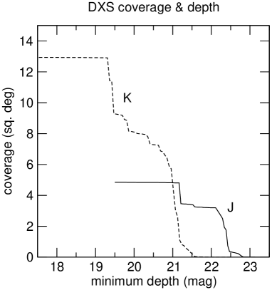
Figure 12: DXS areal coverage attaining a given minimum depth as a function of the minimum depth, for J and K.

Field	Sub-field	RA	Dec	$t_{\rm tot}$ (s)	Depth (mag)	seeing $(\arcsec)$	$t_{\rm tot}$ (s)	Depth (mag)	seeing $(\arcsec)$
		J2000		$J$			$K$
XMM-LSS	1.00	36.5752020	-4.7496444	5760	22.26	0.88	6400	20.83	0.72
XMM-LSS	1.10	36.5803542	-4.5294528	6400	22.28	0.86	6400	20.87	0.74
XMM-LSS	1.01	36.8012000	-4.7496444	5760	22.24	0.84	6400	20.82	0.73
XMM-LSS	1.11	36.8012000	-4.5294528	5760	22.27	0.85	3840	20.62	0.71
XMM-LSS	2.00	35.7098417	-4.7496444	-	-	-	5760	20.59	0.92
XMM-LSS	2.10	35.7098417	-4.5294528	-	-	-	4480	20.54	0.86
XMM-LSS	2.01	35.9306875	-4.7496444	-	-	-	4480	20.50	0.84
XMM-LSS	2.11	35.9306875	-4.5294528	-	-	-	5120	20.55	0.84
Lockman Hole	1.00	163.3623000	57.4753556	-	-	-	11460	20.94	0.93
Lockman Hole	1.10	163.3623000	57.6955472	-	-	-	10320	20.90	0.94
Lockman Hole	1.01	163.7756167	57.4753556	-	-	-	9180	20.85	0.93
Lockman Hole	1.11	163.7756167	57.6955472	-	-	-	9180	20.86	0.95
Lockman Hole	6.00	161.6707620	59.1223000	-	-	-	4500	20.52	1.03
Lockman Hole	6.10	161.6707620	59.3424917	-	-	-	2500	20.23	0.93
Lockman Hole	6.01	162.1040380	59.1223000	-	-	-	4000	20.48	1.01
Lockman Hole	6.11	162.1040380	59.3424917	-	-	-	3500	20.42	1.02
ELAIS N1	1.00	242.5994000	54.5031333	2000	21.39	0.97	3000	20.25	0.93
ELAIS N1	1.10	242.5994000	54.7233250	2000	21.41	0.94	4000	20.44	0.95
ELAIS N1	1.01	242.9817370	54.5031333	3640	21.64	0.96	3500	20.38	0.94
ELAIS N1	1.11	242.9817370	54.7233250	2420	21.31	0.97	2500	20.17	0.95
VIMOS 4	1.00	334.2667460	0.1698000	7680	22.24	0.87	7340	20.74	0.81
VIMOS 4	1.10	334.2667460	0.3899917	9600	22.40	0.85	11540	20.96	0.78
VIMOS 4	1.01	334.4869460	0.1698000	8960	22.38	0.82	10260	20.94	0.80
VIMOS 4	1.11	334.4869460	0.3899917	5120	22.06	0.88	7480	20.75	0.83
VIMOS 4	2.00	335.1420250	0.1817444	3200	21.72	0.86	7680	20.86	0.73
VIMOS 4	2.10	335.1420250	0.4019361	3840	21.80	0.89	7680	20.86	0.70
VIMOS 4	2.01	335.3622250	0.1817444	2560	21.54	0.90	7040	20.80	0.70
VIMOS 4	2.11	335.3622250	0.4019361	4480	21.87	0.90	7040	20.76	0.72
VIMOS 4	3.00	335.1420790	1.0559111	-	-	-	4480	20.42	0.87
VIMOS 4	3.10	335.1420790	1.2761028	-	-	-	5760	20.54	0.89
VIMOS 4	3.01	335.3623330	1.0559111	-	-	-	4480	20.44	0.88
VIMOS 4	3.11	335.3623330	1.2761028	-	-	-	7040	20.68	0.87
VIMOS 4	4.00	334.2668040	1.0559111	-	-	-	1920	19.95	0.86
VIMOS 4	4.10	334.2668040	1.2761028	-	-	-	3200	20.16	0.87
VIMOS 4	4.01	334.4870580	1.0559111	-	-	-	3200	20.26	0.92
VIMOS 4	4.11	334.4870580	1.2761028	-	-	-	3840	20.32	0.92

Table 5: The DXS deepleavstack multiframes. The field, sub-field code, and base coordinates, are listed, followed by the total integration time in seconds and the 5$\sigma$ point source sensitivity in J and in K.

5.3.1 Deep ExtraGalactic Survey

All the intermediate stack frames from 05A and 05B that pass QC have been included in DR1. However the most important products are the deepleavstack frames. The EDR for the DXS included all the 05A data, and 05B data taken up to 2005 September 27. Therefore for some of the deep tiles (e.g. in ELAIS N1) there are no new observations included in DR1. However the QC and stacking procedures have evolved since the EDR, so the DR1 stacks supersede any EDR stacks. As already noted the stacking of deepleavstack frames for the EDR was less than optimal.

In DR1 there are nine deep tiles in the K band, giving 36 deepleavstack multiframes, since there is one such frame per detector. There are four deep tiles in the J band, which are a subset of the K tiles, and give 16 deepleavstack multiframes. Details of all the DXS deepleavstacks are provided in Table 5. The first column provides the field name, and the second is a code identifying the sub-field, in the form Tile.XY, where XY are binary coordinates specifying one of four multiframe positions that make up a tile. Columns three and four provide the coordinates of the base position, which is the centre of the field of view (which is a point not imaged by the detectors). The remaining columns give the total integration time $t_{\rm tot}$ of the frames contributing to the stack (i.e. excluding deprecated frames), and the $5\sigma$ depth, for the J and K frames.

Fig. 12 illustrates the distribution of depths of the DXS observations in the DR1+ database, plotting the summed area that attains a given minimum depth.

5.3.2 Ultra Deep Survey

Band	$t_{\rm tot}$	Depth	seeing
	s	5$\sigma$	$\arcsec$
$J$	21060	22.61	0.86
$K$	33910	21.55	0.76

Table 6: UDS deep stacks. The table lists the total integration time in seconds, the 5$\sigma$ point source depth, and the image FWHM, in the J and K bands.

As already noted, for the UDS the EDR included data taken up to 2005 September 27. The DR1 includes additional observations, and the new stacked images reach substantially deeper. The total integration times on source, and depths reached in $J$ and $K$, and the seeing, are summarised in Table 6. As explained in Section 3 the UDS data are mosaiced. The individual $3\times 3$ microstepped detector frames are resampled onto a $\sim 24000\times 24000$ pixel grid, and the data are then stacked. In the WSA, the final frame is referred to as a mosaicdeepleavstack frame. Unlike all other stacked data in the WSA, astrometry of the deep UDS stacks uses tangential projection (TAN) rather than the zenith polynomial projection (ZPN) that is standard for WFCAM.

5.4 Survey status summary

We have estimated the percentage completion of the surveys relative to the final 7-year goals set out in Lawrence et al. (2006), by computing the product over all filters of the area covered and the summed effective integration times (established from the depth achieved), in the DR1+ database. Computed in this way the completeness of the surveys is as follows: LAS 6 per cent, GPS 7 per cent, GCS 13 per cent, DXS 11 per cent, UDS 4 per cent. Overall, DR1 marks completion of 7 per cent of the UKIDSS final goals.

Acknowledgements

We are grateful to Roc Cutri for several helpful discussions.

References

- (1)
- Abazajian et al. (2003) Abazajian, K., et al., 2003, AJ, 126, 2081
- Bertin & Arnouts (2002) Bertin, E., Arnouts, S., 1996, A&A, 117,393
- Bertin et al. (2002) Bertin, E., Mellier, Y., Radovich, M., Missonnier, G., Didelon, P., Morin, B., 2002, ‘Astronomical Data Analysis Software and Systems XI ’, ASP Conference Proceedings, Vol. 281, p. 228. Eds. D. A. Bohlender, D. Durand, & T. H. Handley.
- Casali et al. (2006) Casali, M., et al., 2006, A&A, in press
- Dye et al. (2006) Dye, S., Warren, S. J., Hambly, N. C., et al., 2006, MNRAS, 372, 1227
- Foucaud et al. (2006) Foucaud, S., et al., 2006, in prep.
- Hewett et al. (2006) Hewett, P. C., Warren, S. J., Leggett, S. K., & Hodgkin, S. T. 2006, MNRAS, 367, 454
- Lawrence et al. (2006) Lawrence, A., et al., 2006, MNRAS, submitted (astro-ph/0604426)
- Nikolaev et al. (2000) Nikolaev, S., Weinberg, M. D., Skrutskie, M. F., Cutri, R. M., Wheelock, S. L., Gizis, J. E., Howard, E. M., 2000, AJ, 120, 3340
- Patat (2003) Patat, F. 2003, A&A, 400, 1183
- Stoughton et al. (2002) Stoughton C., et al., 2002, AJ, 123, 485
- Ungerechts & Thaddeus (1987) Ungerechts, H., Thaddeus, P., 1987, ApJS, 63, 645