WFCAM, Spitzer-IRAC and SCUBA observations of the massive star forming region DR21/W75: I. The collimated molecular jets

Abstract

We present wide-field near-infrared images of the DR21/W75 high-mass star forming region, obtained with the Wide Field Camera, WFCAM, on the United Kingdom Infrared Telescope. Broad-band JHK and narrow-band H₂ 1-0S(1) images are compared to archival mid-IR images from the Spitzer Space Telescope, and 850µm dust-continuum maps obtained with the Submillimeter Common User Bolometer Array (SCUBA). Together these data give a complete picture of dynamic star formation across this extensive region, which includes at least four separate star forming sites in various stages of evolution. The H₂ data reveal knots and bow shocks associated with more than 50 individual flows. Most are well collimated, and at least five qualify as parsec-scale flows. Most appear to be driven by embedded, low-mass protostars. The orientations of the outflows, particularly from the few higher-mass sources in the region (DR21, DR21(OH), W75N and ERO 1), show some degree of order, being preferentially orientated roughly orthogonal to the chain of dusty cores that runs north-south through DR21. Clustering may inhibit disk accretion and therefore the production of outflows; we certainly do not see enhanced outflow activity from clusters of protostars. Finally, although the low-mass protostellar outflows are abundant and widely distributed, the current generation does not provide sufficient momentum and kinetic energy to account for the observed turbulent motions in the DR21/W75 giant molecular clouds. Rather, multiple epochs of outflow activity are required over the million-year timescale for turbulent decay.

1 Introduction

Star formation studies have in recent years benefited from a fresh, “large scale” view, via observations of Giant Molecular Clouds (GMCs) and large clusters of clumps and cores at infrared and (sub)millimetre wavelengths, and through studies of the interplay between the thousands of evolving young sources within each region.

Infrared survey instrumentation that offers an unparalleled field of view at high spatial resolution is now, or will soon be, available at modest-sized telescopes across the globe. One such instrument is the near-infrared (near-IR) Wide Field Camera, WFCAM, at the U.K. Infrared Telescope (UKIRT). WFCAM provides deep imaging of degree-sized regions in broad and narrow-band filters in just a few hours. When combined with photometric data at longer wavelengths, e.g. from the Submillimeter Common User Bolometer Array (SCUBA - soon to be replaced by SCUBA-2) and the Spitzer Space Telescope, obtaining a complete picture of evolving star formation (stellar populations, the IMF, the clump mass function, etc.) becomes possible. Complementary wide-field optical images of Herbig-Haro (HH) jets, and future large-scale (sub)millimetre surveys of molecular “CO” outflows, may also be used to examine the dynamic processes that shape – through the injection of turbulence or triggered cloud collapse – star formation across each GMC.

One region that has already benefited from wide-field observations with Spitzer, SCUBA and now WFCAM is the DR21/W75S, DR21(OH) and W75N complex of massive star forming cores in Cygnus X (Westerhout, 1958; Downes & Rinehart, 1966, for a more recent overview of the Cygnus X complex of GMCs see Schneider et al. 2006). The DR21 core contains two well-studied cometary Hii regions (Harris, 1973; Dickel et al., 1986; Cyganowski et al., 2003) and an H₂O maser (Genzel & Downes, 1977), while DR21(OH), a dense core roughly 3′ to the north of DR21, is abundant with methanol, water and OH masers (Liechti & Walmsley, 1997, and references therein). DR21(OH) is undetected in radio continuum emission and so is probably younger than DR21. W75N, roughly 20′ to the north of DR21, comprises a group of embedded infrared sources (Moore et al., 1991b; Persi, Tapia & Smith, 2006), Hii regions and compact radio sources (e.g. Haschick et al., 1981; Hunter et al., 1994), as well as H₂O and OH masers (Hunter et al., 1994; Torrelles et al., 1997).

Early work by Dickel et al. (1978) and Fischer et al. (1985) showed that DR21 and W75N coincide with two, possibly interacting molecular cores along a north-south molecular ridge extending over at least half a degree. These cores, evident in the more recent 850 $\mu$m dust continuum maps of Vallée & Fiege (2006) and Gibb et al. (2007), have been resolved into smaller clumps by various groups (Wilson & Mauersberger, 1990; Mangum, Wooten & Mundy, 1992; Chandler, Gear & Chini, 1993a; Shepherd, 2001). Spitzer images at 5.8 and 8.0 $\mu$m reveal streamers of emitting material that seem to radiate away from the brighter infrared sources located along the molecular ridge (Marston et al., 2004), features possibly produced by ionization and ablation of the less dense material on either side of the ridge. Marston et al. (2004) also identify a number of “extremely red objects”, or EROs, along the ridge. These are luminous, highly-reddened objects that may be very young, massive, early B-type sources.

In terms of outflows, DR21 and W75N have been studied independently by a number of groups. DR21 drives one of the most spectacular flows known (Garden et al., 1991b; Garden & Carlstrom, 1992). The bipolar outflow is extremely bright in H₂ line emission (Garden et al., 1991a; Davis & Smith, 1996; Smith, Eislöffel & Davis, 1998) and produces methanol abundance enhancements and masers through shocks (Liechti & Walmsley, 1997). The dominant outflow from W75N is somewhat fainter in H₂, although it appears to be a good example of a wind-driven flow, in which sweeping bow shocks entrain ambient gas to form a massive molecular outflow (Davis et al., 1998a; Davis, Smith & Moriarty-Schieven, 1998b). Early CO maps showing the orientation and bipolarity of the W75N outflow were presented by Fischer et al. (1985); more detailed maps in CO and millimetre continuum emission by Shepherd (2001), Shepherd, Testi & Stark (2003) and Shepherd, Kurtz & Testi (2004) illustrate the complexity of the region.

In this paper we discuss WFCAM data obtained in H₂ 1-0S(1) emission and in the J, H and K bands. The images cover a 0.8°$\times$ 0.8° “tile” (see Section 2) centred close to DR21. The broad-band photometry are discussed in detail in a companion paper (Kumar et al., 2006, hereafter Paper II); in this work we focus on the H₂ emission-line features associated with the many outflows along the DR21/W75N ridge. A comparison is also made with SCUBA 850 $\mu$m data (see also Vallée & Fiege (2006) and Gibb et al. (2007) for a similar map), and archival Spitzer IRAC images at 3.6 $\mu$m, 4.5 $\mu$m, 5.8 $\mu$m and 8.0 $\mu$m (originally presented by Marston et al., 2004). The combined SPITZER and SCUBA maps suggest that stars are forming within a flattened north-south filament viewed almost edge on. One of the goals of the WFCAM observations was to search for outflows ejected east-west, i.e. perpendicular to this dense filament. We discuss the effect these outflows might have on the general GMC, and look for examples of collimated jets from the more massive YSOs.

There has been some disagreement on the distance to DR21 and W75N, although both are thought to be in the range 1.5-3.0 kpc (Genzel & Downes, 1977; Fischer et al., 1985; Odenwald & Schwartz, 1993; Schneider et al., 2006). In Paper II we find that the upper limit gives a more realistic population of massive stars, so we adopt 3 kpc as a general distance in this paper.

2 Observations

2.1 WFCAM and Spitzer imaging

Wide-field images of the DR21/W75 region were obtained during service observing at the United Kingdom Infrared Telescope (UKIRT) on 6 May, 11 May and 9 June 2005, using the near-IR wide-field camera WFCAM (Casali et al., 2006). The camera employs four Rockwell Hawaii-II (HgCdTe 2048x2048) arrays spaced by 94% in the focal plane. The pixel scale measures 0.40″.

To fill in the gaps between the arrays, and thereby observe a contiguous square field on the sky covering 0.75 square degrees – what is referred to as a WFCAM “tile” – observations at four positions are required. At each position, to correct for bad pixels and array artifacts, a five-point jitter pattern was executed (with offsets of 3.2″ or 6.4″); to fully sample the seeing, at each jitter position, a 2x2 micro-stepped pattern was also used, with the array shifted by half a pixel. In this way 20 frames were obtained at each of the four positions in the tile.

Data through Mauna Kea Consortium broad-band J, H and K filters, and a narrow-band H₂ 1-0S(1) filter ($\lambda=2.121$ $\mu$m, $\delta\lambda=0.021$ $\mu$m), were obtained (Hewett et al., 2006). Exposure times of 5 sec and 40 sec were used with the broad and narrow-band filters, respectively. A correlated double sampling (CDS) readout mode was used with the broad-band filters, while a non-destructive readout (NDR) mode was employed with the longer-exposure H₂ images. The latter yields a lower read noise ($\sim$20e- as compared to $\sim$30e- with CDS) at the expense of greater amplifier glow and a higher risk of electronic pickup. With the 5-point jitter pattern and 2x2 micro-stepping in each broad-band filter, the total on-source/per-pixel integration time was 100 sec per filter. In H₂ the whole 20-frame sequence was repeated; hence, the total per-pixel exposure time was 1600 sec.

The data were reduced by the Cambridge Astronomical Survey Unit (CASU), which is a fore-runner to the VISTA Data Flow System Project (VDFS), a collaborative effort between the Universities of London, Cambridge and Edinburgh in the U.K. CASU is responsible for the design and implementation of the data processing pipeline used prior to the archiving and subsequent distribution of all WFCAM data. The reduction steps are described in detail by Dye et al. (2006) and Irwin et al. (2006). Briefly, dark frames secured at the beginning of the night were subtracted from each target frame to remove bad pixels, amplifier glow, and reset anomalies from the raw frames. Twilight flats were then used to flat-field the data. The micro-stepped frames were interleaved and the offset frames combined by weighted averaging (using a confidence map derived largely from the flat-field frames) to produce “leavestack” frames.

Astrometric calibration was achieved through a cubic radial fit and a six-parameter linear transformation to objects found in the 2MASS point source catalogue (Dye et al., 2006). The transformation takes into account translation, scaling, rotation and shear. Photometric calibration was also achieved through the use of 2MASS data (Dye et al., 2006; Hewett et al., 2006).

All reduced WFCAM data are archived at the WFCAM Science Archive (WSA), which is part of the Wide Field Astronomy Unit (WFAU) hosted by the Institute for Astronomy at the Royal Observatory, Edinburgh, U.K. (http://surveys.roe.ac.uk/wsa/index.html). WSA data are distributed as RICE-compressed Multi-Extension Fits (MEF) files. The data for one filter covering the 0.8^∘$\times$0.8^∘ tile appear as four leavestack files in the database, one MEF file for each of the four offsets on sky needed to cover the tile. Each leavestack file therefore contains four individual images, one for each of the four WFCAM cameras.

Having retrieved the reduced data from the WFCAM Science Archive (WSA), Starlink software were used to remove residual large-scale gradients across each of the 16 images in each tile. The Starlink:KAPPA command SURFIT was used to fit a coarse surface to the background in each frame; the four surface fit images in each corner of the full tile were median-averaged and used to flat-field the four associated target frames. The frames were subsequently mosaicked together using the KAPPA:WCSALIGN routine applied to the world coordinates assigned to each frame by the CASU pipeline, together with the Starlink:CCDPACK mosaicking routine MAKEMOS. These gave one complete tile image in each filter.

The Spitzer Space Telescope images discussed in this paper were retrieved from the Spitzer archive. Our processing of these data is described in Paper II. The observations were obtained with the IRAC camera, which is described by Fazio et al. (2004). The data also appear in recent papers by Marston et al. (2004) and Persi, Tapia & Smith (2006), although Marston et al. (2004) only give preliminary results, while Persi, Tapia & Smith (2006) focus only on a small $\sim$2′$\times$2′ field centred on W75N.

2.2 SCUBA observations

The sub-millimetre data were obtained with the SCUBA bolometer array camera (Holland et al., 1999) on the James Clerk Maxwell Telescope (JCMT) on Mauna Kea, Hawaii on four partial nights from May 26 to May 29, 2001 in marginal sub-millimetre conditions; the precipitable water vapor (PWV) was $\sim$1.3–2 mm (optical depth at 850 $\mu$m $\sim$0.25–0.36), although it was fairly stable each night. Due to the high PWV content in the atmosphere only the 850 $\mu$m data were usable. The standard “scan-mapping” mode (Jenness, Lightfoot & Holland, 1998) was employed with six different chop throws: 30″, 44″, and 68″ in Right Ascension and Declination respectively, while scanning in the Nasmyth coordinate frame. Each chop throw was repeated 2–4 times depending on airmass and sky opacity, the goal being to reach the same noise level in each dual beam map. The rms noise level in the final co-added dual beam maps was $\sim$0.09–0.1 Jy beam^-1. The pointing was checked frequently on the point source MWC 349, and each dual beam map was corrected for any pointing drift between pointing observations. Based on the pointing data the positional accuracy in the final 850 $\mu$m image is estimated to be $\leq$1″. The maps were calibrated with scan maps of Uranus as the primary flux calibrator and CRL 2688 as the secondary calibrator. The flux calibration is estimated to be good to within 5% with respect to Uranus. The telescope half power beam width was measured to be 15.2″ from scan maps of Uranus.

The maps were reduced in a standard way using the Starlink reduction packages SURF and Kappa (Sandell, Jessop & Jenness, 2001), except that the individual dual beam maps where created by weighting the noise in each individual bolometer using the SURF task setbolwt, which reduced the noise level in the maps by $\sim$5–10% . We then estimated the rms noise level using emission free areas in the maps and co-added the maps by accounting for the difference in noise between individual maps for the same chop throw and chop position angle. The final calibrated 850 $\mu$m map has a noise level of 50–60  Jy beam^-1 over the whole area. For further analysis we divided the map into three areas (south, middle, and north), removed the error beam using the MIRIAD task CLEAN (Sault, Teuben & Wright, 1995) and restored the maps to 14.0″ resolution. Below we present only photometry of the major 850 $\mu$m cores, plus contour maps for comparison with the near- and mid-IR data. A more thorough analysis of the 850 $\mu$m observations is beyond the scope of this paper, and will be presented in a later work.

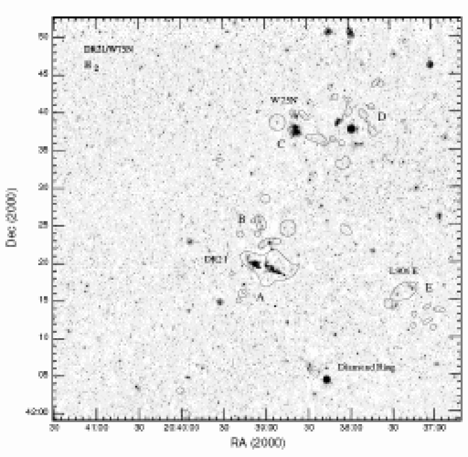
Figure 1: A near-IR narrow-band H₂ 2.122 $\mu$m image of the DR21 and W75N regions. The figure shows a full WFCAM tile, covering an area of roughly 0.8$\times$0.8 degrees. Areas were H₂ line emission is identified are outlined; the regions A, B, C, D and E are discussed separately in Sect. 4.

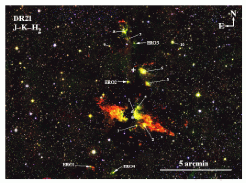
Figure 2: A colour image of the DR21 region composed of observations in J (blue), K (green) and H₂ (red). With this combination H₂ line emission regions appear red, while embedded or background stars appear yellow. The star and triangle mark the DR21 A-B-C and DR21 D cometary Hii regions; the cross indicates the location of the DR21(OH) cluster of water, methanol and OH masers (Liechti & Walmsley, 1997). EROs identified by Marston et al. (2004) are labeled; the infrared “DR21-IRS” sources discussed in the text are numbered.

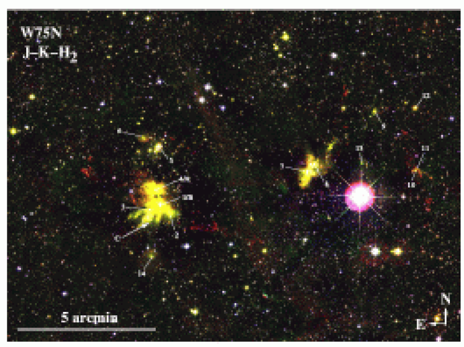
Figure 3: Same as Fig. 2, except for the region around W75N. The bright infrared sources referred to as W75N-IRS 1, etc. in the text are numbered. The letters A, B and C refer to the main Hii regions.

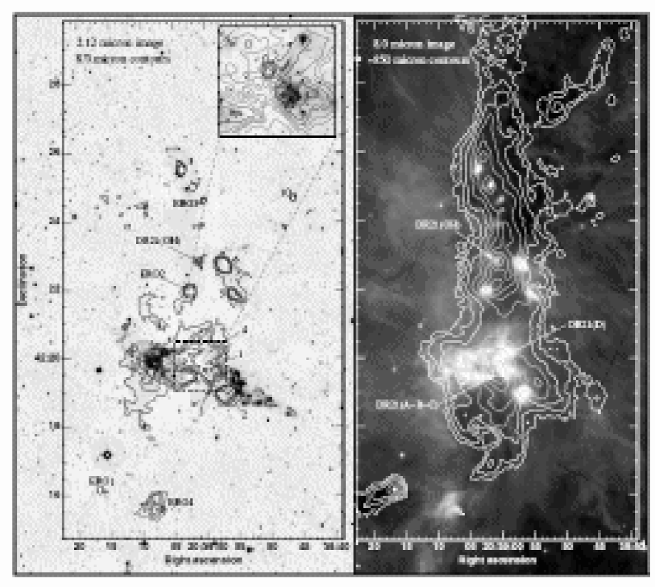
Figure 4: Left: WFCAM H₂ 2.12 $\mu$m image of DR21 with Spitzer IRAC 8.0 $\mu$m contours overlayed. The contours pick out only the brightest 8.0 $\mu$m peaks; lower contours associated with diffuse PAH emission are not plotted. Contour levels are 3.4, 5.1, 6.8, 10.2 mJy arcsec^-2 (black) and 17.0, 30.6, 85.0, 165.0 mJy arcsec^-2 (white); inset, the same contours are plotted but with thin and thick lines. DR21-IRS sources are numbered. Right: Spitzer IRAC 8.0 $\mu$m image with SCUBA 850 $\mu$m contours overlayed. Contour levels are 0.125, 0.25, 0.5, 1, 2, 4, 8 and 16 Jy/beam; the beam size measures 14″.

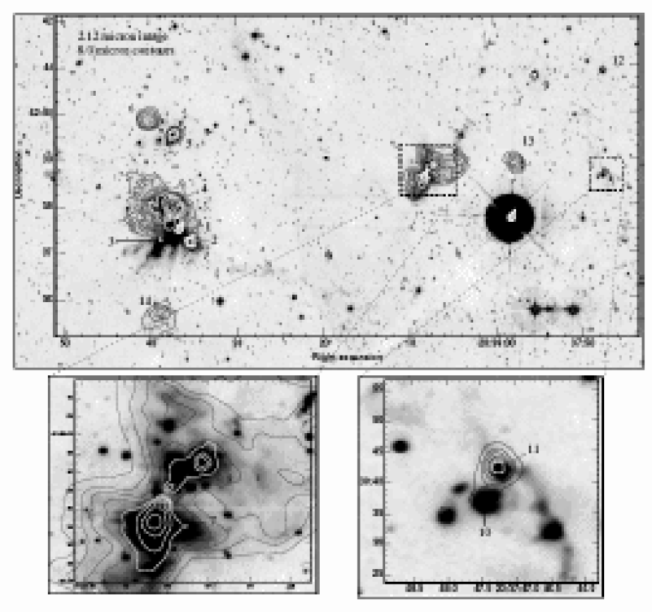
Figure 5: WFCAM H₂ 2.12 $\mu$m image of W75N and the northwest, with Spitzer IRAC 8.0 $\mu$m contours overlayed. Contour levels are 3.4, 5.1, 6.8, 10.2 mJy arcsec^-2 (black) and 17.0, 30.6, 85.0, 165.0 mJy arcsec^-2 (white). The W75N-IRS sources are numbered.

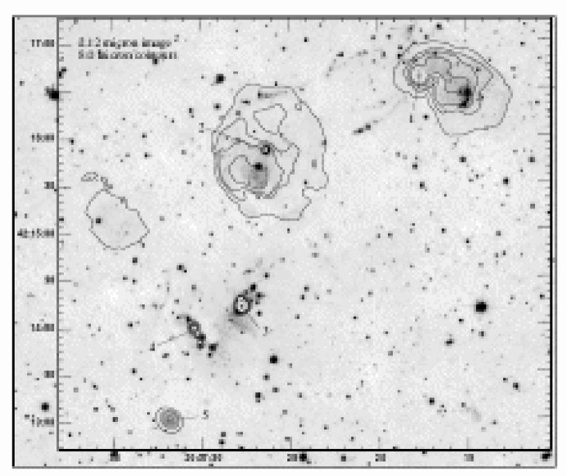
Figure 6: WFCAM H₂ 2.12 $\mu$m image of the eastern edge of L906 (west of DR21). Spitzer IRAC 8.0 $\mu$m contours are overlayed. Contour levels are 3.4, 5.1, 6.8, 10.2 mJy arcsec^-2 (black) and 17.0, 30.6, 85.0, 165.0 mJy arcsec^-2 (white). The L906E-IRS sources are numbered.

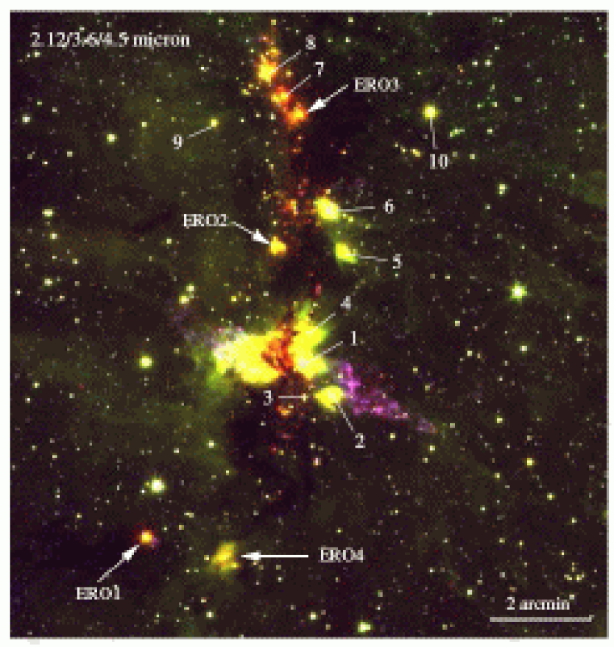
Figure 7: Colour image constructed from WFCAM H₂ data (2.12 $\mu$m - blue) and Spitzer IRAC images (3.6 $\mu$m - green; 4.5 $\mu$m - red). EROs are labeled and DR21-IRS sources are numbered.

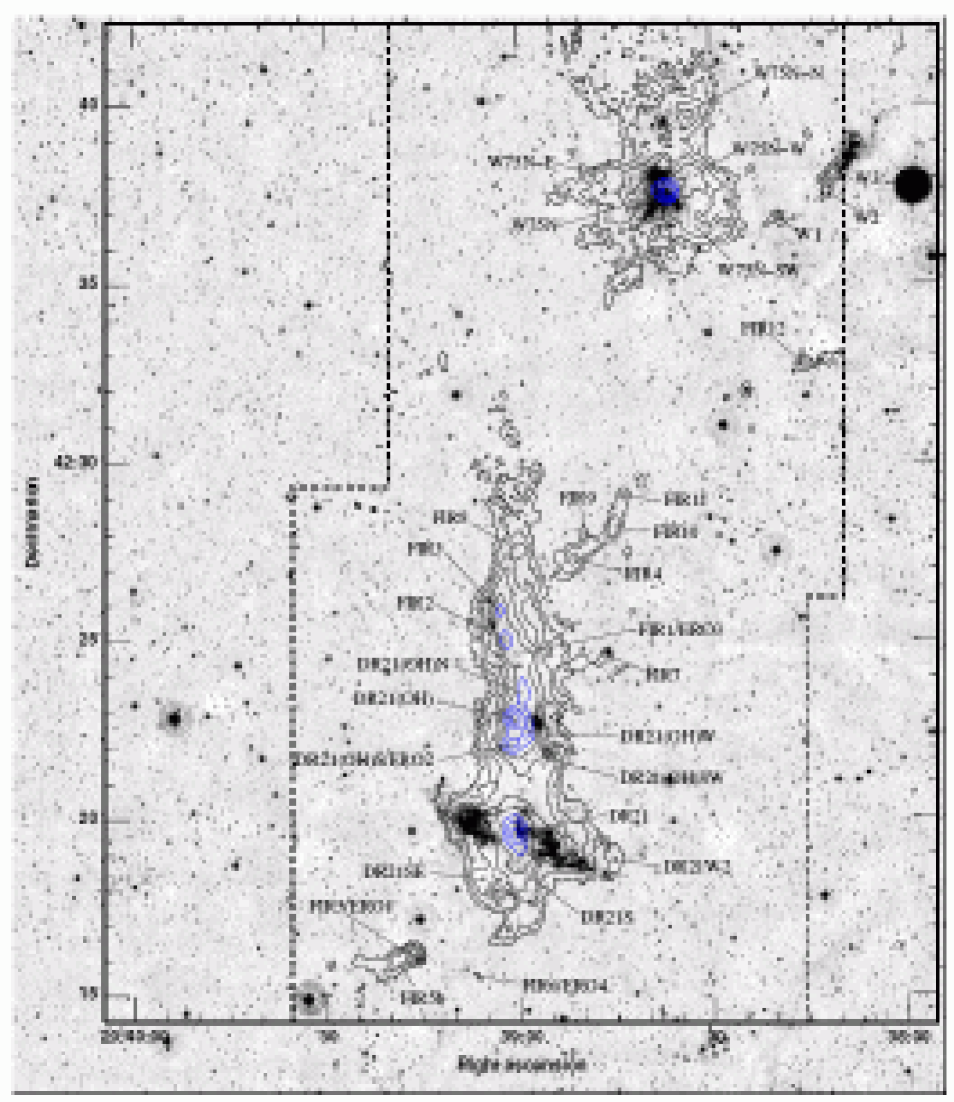
Figure 8: WFCAM H₂ image of a portion of the DR21/W75 tile with, superimposed, contours of the 850 $\mu$m emission. The SCUBA contours represent 0.125, 0.25, 0.5, 1, 2, 4, 8 and 16 Jy/beam (the beam size measures 14″ at 850 $\mu$m). The extent of the SCUBA map is marked with dashed lines.

3 Results

3.1 WFCAM imaging of DR21/W75

Our H₂ 1-0S(1) (+ continuum) tile of the DR21/W75 region is presented in Fig.1 (which shows the full field observed). Regions where H₂ line-emission features were identified have been outlined. Although somewhat clustered around DR21 and W75N, these generally follow the ridge of obscuration that links DR21 in the centre with W75N in the north-northwest. There is also a cluster of features to the west-south-west of DR21, which may be unrelated to the main high-mass star forming ridge.

Colour images of the regions around DR21 and W75N are shown in Figs. 2 and 3. J, K and H₂ mosaics were scaled by exposure time, filter bandpass and filter transmission before being registered and combined. In the resulting figures embedded sources can be easily distinguished from pure line-emission features, i.e. the H₂ knots and bow shocks in jets and outflows. The former appear yellow while the latter are bright red in colour. Some of the yellow features in the DR21 lobes are due to scattered continuum, while some may result from “boosted” K-band emission due perhaps to enhanced vibrational excitation by fluorescence (Fernandez, Brand & Burton, 1997). Many of the features marked in Fig. 1 are seen in more detail here; indeed, these colour images were used to search for H₂ features across this extensive region. In Fig. 2 the molecular ridge that runs through the middle of DR21 is evident as a dark lane, largely devoid of point sources. We mark on Fig. 2 the “Extremely Red Objects”, or EROs, identified by Marston et al. (2004), as well as the location of the DR21 A-B-C and D Hii regions (Cyganowski et al., 2003), and the DR21(OH) cluster of water, OH and methanol masers (Liechti & Walmsley, 1997). In Fig. 3 the Hii regions A, B and C in W75N (Haschick et al., 1981) are labeled. In both figures K-band sources with bright 8.0 $\mu$m counterparts are numbered; these are probably the most massive, embedded sources in the region.

DR21 is famous for its Hii regions. It comprises four main radio emission peaks, originally labeled A, B, C and D (Harris, 1973; Roelfsema, Goss & Geballe, 1989). None of the radio peaks are detected in the near-IR (Davis & Smith, 1996), although the northern, compact source D is observed at mid-IR wavelengths. Smith et al. (2005) point to this source as being the dominant source of infrared luminosity in DR21. They find that its total luminosity exceeds that of an O8 ZAMS star and attribute the excess to accretion. They estimate an extinction of $A_{\rm v}\sim 175$ mag toward source D, and suggest that because it is still accreting, it could (at least in part) be responsible for the large-scale DR21 outflow. However, at radio wavelengths Hii region D is cometary in appearance, opening outward toward the north (Cyganowski et al., 2003). One could argue that a north-south flow is more likely. Either way, there are no H₂ knots or jet-like features close to this source which one might confidently associate with the Hii region.

Situated $\sim$20″ south of source D, radio sources A, B and C appear to be peaks in a larger “bow shock” or “champagne flow” style cometary nebula (Cyganowski et al., 2003). This nebula lies $\sim$15″ to the east of the cluster of near-IR sources in DR21, within the dark lane that separates the two lobes of the DR21 outflow. It is coincident with a dense molecular core (see Section 3.3), although it has no mid-IR counterpart. Overall, the cometary A-B-C nebula opens in the direction of the eastern lobe of the main DR21 outflow. This might suggest a causal relationship between the flow and the Hii region. However, the more collimated, western lobe of the DR21 outflow is difficult to reconcile with the sharp, western edge of the cometary Hii region. The powerful flow would surely disrupt this Hii region/molecular cloud boundary, if the outflow central engine was situated within the cometary nebula.

The complex of masers and mm-wave continuum peaks known as DR21(OH) are found about 3′ to the north of DR21 (A-B-C-D). DR21(OH) coincides with a chain of four water masers (Forster et al., 1978; Mangum, Wooten & Mundy, 1992) spread northeast-southwest over about 20″. Orthogonal to the water masers, about a dozen methanol masers delineate the two lobes of the DR21(OH) outflow (Plambeck & Menten, 1990; Kogan & Slysh, 1998). The water masers likely trace embedded young stars and ultra-compact Hii regions, including in this case the outflow central engine, while the class I methanol masers probably trace the interaction between the outflow and the ambient medium. H₂ line emission is also excited in such outflow-ambient impact zones, although we fail to detect clear evidence for H₂ emission in our WFCAM data. The absence of H₂ emission in the DR21(OH) outflow is likely due to extinction.

W75N, shown in Fig. 3, comprises three regions of radio emission, W75N(A), W75N(B) and W75N(C) (Haschick et al., 1981). A and B are coincident with patches of bright near-IR nebulosity; the more evolved source, W75N(A), is associated with a 2 $\mu$m point source. The overall cluster harbours at least 30 IR sources with infrared excesses, probably due to circumstellar disks (Moore et al., 1991b; Persi, Tapia & Smith, 2006).

Collectively, W75N is associated with a $\sim 10^{3}$ M_⊙ dense molecular core (Moore et al., 1991a), which Shepherd, Testi & Stark (2003) resolve into nine discrete millimetre continuum peaks spread over an area of about an arcminute. The brightest and most massive, MM 1, peaks a few arcseconds to the northwest of IRS 1 and is associated with Hii region W75N(B); W75N(A) is similarly associated with a continuum peak, MM 5. MM 1 contains at least four Hii regions (a fifth is associated with MM 5). Three of these were detected at 1.3 mm with the VLA by Torrelles et al. (1997). Of these, VLA 1 drives a radio jet in the direction of the large-scale molecular outflow, although all three VLA sources may drive independent flows (Shepherd, 2001; Shepherd, Testi & Stark, 2003). All three sources are associated with water maser emission (Torrelles et al., 1997); VLA 1 is also surrounded by a compact cluster of OH masers (Baart et al., 1986; Hutawarakorn, Cohen & Brebner, 2002). Each source is presumably in the protostellar phase, their radio fluxes being consistent with early B-type ZAMS stars. Indeed, Shepherd, Kurtz & Testi (2004) assign spectral types of B0-B2 to all five Hii regions, W75N(A) being perhaps the most evolved at B0.5. Our H₂ observations of W75N reveal not only the well-known H₂ features associated with W75N itself, but also collimated jets to the north and west.

Lastly, roughly 15′-20′ to the west of DR21 there is a further region of active star formation that has to date attracted little attention. The region is evident in the Spitzer data of Marston et al. (2004), although they do not discuss these features in any detail. A search of the SIMBAD database suggests that the region is situated on the eastern edge of the small L906 dark cloud. We find an abundance of H₂ line emission knots and jets, plus regions of bright, nebulous, mid-IR emission and a number of highly reddened sources (Paper II). We use the suffix L906E for the sources in this region.

Notably, no H₂ flows were found in the Diamond Ring region (Fig. 1), which is consistent with this area being more evolved than DR21, W75N and L906E.

3.2 Comparison with Spitzer data

3.2.1 The young stars

In Figs. 4–6 we compare our WFCAM observations of DR21/W75 with the archival Spitzer 8.0 $\mu$m observations first discussed by Marston et al. (2004) and Persi, Tapia & Smith (2006). These longer-wavelength data are potentially very useful for tracing luminous, embedded sources. Photometry of the brighter 8.0 $\mu$m point sources is given in Table LABEL:irs.

The EROs identified by Marston et al. (2004) in DR21 are bright, reddened 8 $\mu$m sources with spectral indices ($\alpha=d{\rm log}\lambda F_{\lambda}/d{\rm log}\lambda$) between 2.2 $\mu$m and 8.0 $\mu$m in the range 1.8 to 3.6, much larger than the $\alpha>0.3$ lower limit for Class I protostars (Lada, 1987). ERO 1 lies at the western edge of an “infrared dark cloud” that extends eastward for at least 2′ (Marston et al., 2004); the cloud is evident as a region devoid of stars in Fig. 2. In the 850 $\mu$m data described below the cloud is seen as two peaks (FIR 5 and FIR 5b) enveloped in an easterly elongation of the dust emission.

The other extremely red objects, ERO 2, ERO 3 and ERO 4, all lie along the north-south chain of dense cores that runs through the centre of DR21. In Table LABEL:irs we list the Spitzer magnitudes of these and many other bright 8.0 $\mu$m sources in DR21/W75: in Fig. 4 (around DR21), Fig. 5 (near to W75N) and Fig. 6 (around L906E), these sources are labeled DR21-IRS 1, DR21-IRS 2, etc., W75N-IRS 1, W75N-IRS 2, etc, and L906E-IRS 1, L906E-IRS 2, etc, respectively (the same sources are labeled in the near-IR images in Figs. 2 and 3). These “IRS” sources are generally bright 8.0 $\mu$m point sources or luminous, reddened K-band sources associated with bright 8.0 $\mu$m emission (surface brightness $>$7 mJy arcsec^-2). All appear as peaks or discrete sources in Figs. 4-6. Spectral indices, $\alpha$, derived from linear fits to the Spitzer photometry between 3.6 $\mu$m and 8.0 $\mu$m (as described in Paper II), are also given in Table LABEL:irs. We do not correct for extinction since this is not know a priori for each source, although it is worth noting that, at a distance of 3 kpc the interstellar extinction to DR21/W75 may be as large as $A_{\rm v}\sim 8.8$ mag (Joshi, 2005). Extinction will have the effect of increasing the range of $\alpha$ values (Paper II). For targets with photometry in only two IRAC bands we do not derive values for $\alpha$, since the 8.0 $\mu$m magnitudes may be compromised by deep silicate absorption in these luminous, embedded sources (e.g Gibb et al., 2000).

Most of the targets in Table LABEL:irs are very red. Indeed, when considering all of the sources, the EROs identified by Marston et al. (2004) do not seem to be particularly unique. We find many other examples of extremely red objects. DR21-IRS 5 and L906E-IRS 1 are particularly noteworthy, having $\alpha$ (uncorrected for extinction) of $\sim 4.1$. UCHii region DR21(D) is also very red, as is DR21(OH). For the EROs, the spectral indices in Table LABEL:irs differ somewhat from those reported by Marston et al. (2004), probably because different photometry apertures (and sky annuli) were used with these moderately extended sources. Our Spitzer photometry in the W75N regions matches that reported by Persi, Tapia & Smith (2006), who use a similar photometry aperture to ourselves, reasonably well.

The mid-infrared sources in the W75N region are shown in Fig. 5. The region associated with W75N(A) and (B) is very complex. Ground-based and Spitzer mid-IR photometry of the sources in the immediate vicinity of W75N have been discussed in detail by Persi, Tapia & Smith (2006), although there are additional mid-IR sources to the north and west close to bright infrared nebulae and regions of H₂ line emission. Persi, Tapia & Smith (2006) identify mid-IR counterparts to the near-IR sources W75N-IRS 1, 2 and 3, as well as the VLA 3 UCHii region in MM 1. They derive an extinction of $A_{\rm v}\sim 90$ to VLA 3.

Much like the IRS sources near DR21, around W75N and to the west, the combined WFCAM and Spitzer data reveal nebulous sources which harbour a luminous O or early-B star within a compact cluster of less-luminous sources (e.g. W75N-IRS 1 to W75N-IRS 5, W75N-IRS 7 and probably W75N-IRS 8), as well as examples of single intermediate-mass sources within an almost spherical shell of reflected near-IR light and 8.0 $\mu$m PAH emission (e.g. W75N-IRS 6, IRS 13 and IRS 14).

In Fig. 6 we show WFCAM 2.12 $\mu$m and Spitzer 8.0 $\mu$m data of star forming regions to the west of DR21. The Spitzer data reveal a chain of three spherical cores. As one moves westward along this chain the cores become less diffuse and more centrally peaked at 8.0 $\mu$m: note that the eastern core in Fig. 6 has no 8.0 $\mu$m point source, while L906E-IRS 2 is markedly fainter than L906E-IRS 1. IRS 1 is extremely red (particularly in comparison to L906E-IRS 2; Table LABEL:irs), and is associated with extensive H₂ filaments that probably delineate at least two jets (discussed further in Section A5). If we also include the cluster of YSOs associated with L906E-IRS 3/IRS 4, then we probably have an evolutionary sequence, with L906E-IRS 1 representing the youngest and L906E-IRS 3/IRS 4 the most evolved region.

The bright Spitzer sources and the clustering properties of the embedded stellar population are discussed in more detail in Paper II.

3.2.2 The outflows

In addition to the embedded young stars, Spitzer also detected the main DR21 outflow at 4.5 $\mu$m. In high-mass star forming regions like DR21/W75, distinguishing line-emission jet features from background diffuse dust and PAH emission regions is difficult, even in the relatively PAH-free 4.5 $\mu$m band. With the broad IRAC bands one is not able to “continuum-subtract” the data. One must therefore use colour images as a diagnostic tool. We show such an image in Fig. 7.

As noted by Marston et al. (2004) and more recently by Smith et al. (2006), the main DR21 outflow is detected by Spitzer. Morphologically, the flow is very similar in images at 2.12 $\mu$m and 4.5 $\mu$m. Indeed, Smith et al. (2006) overlay contours of the H₂ 1-0S(1) emission of Davis & Smith (1996) onto a 4.5 $\mu$m image and find an almost exact correlation between the emission-line features in the two bands. Note also that the flow is consistently the same colour (pink) in Fig. 7. Although the IRAC filter at 4.5 $\mu$m encompasses molecular and atomic emission lines from CO (v=1-0 at 4.45-4.95 $\mu$m) and HI Br$\alpha$ (at 4.052 $\mu$m), the unchanging colour along the DR21 outflow in Fig. 7 suggests that the bulk of the 4.5 $\mu$m emission is in fact from the H₂ 0-0S(9) line (at 4.694 $\mu$m). This conclusion is supported by ISO spectroscopy of portions of the DR21 outflow (Smith, Eislöffel & Davis, 1998; Smith et al., 2006).

In shock models, H₂ emission in outflows is predicted to be particularly strong in the 4.5 $\mu$m band, 5–14 times higher than in the 3.6 $\mu$m band (Smith & Rosen, 2005). Smith et al. (2006) find that in outflows $\sim$50% of the flux in the IRAC 3.6 $\mu$m, 4.5 $\mu$m and 5.8 $\mu$m bands is due to H₂ line emission. Smith, Eislöffel & Davis (1998) propose excitation of the H₂ emission in multiple C-type bow shocks. Smith et al. (2006) also note a conspicuous lack of CO, Br$\alpha$ and PAH emission in the ISO spectra.

Most of the “red” H₂ features evident in our WFCAM images (Figs. 2 and 3) are detected by Spitzer, albeit at lower spatial resolution. In Fig. 7 one or two features along the ridge appear somewhat “redder” than other jet features, probably because of increased extinction (note in particular the knot $\sim$1′ north of DR21-IRS 4). This may also explain the brown colouration at the end of the western DR21 flow lobe, although Smith et al. (2006) – who also note this subtle change in colour – mention that a reduced pre-shock velocity or increased pre-shock density may have the same effect.

The Spitzer 5.8 $\mu$m band covers emission from the strong [FeII] line at 5.34 $\mu$m. However, upon examining the 5.8 $\mu$m images (not shown) we found it impossible to distinguish line emission features associated with the outflow from the more intense, filamentary 6.2 $\mu$m PAH emission that pervades the 5.8 $\mu$m data (the 3.6 $\mu$m and 8.0 $\mu$m bands likewise include bright PAH emission at 3.3 $\mu$m and 7.7 $\mu$m). Suffice to say that no bright [FeII] component was found in the main DR 21 outflow.

Table 1: Catalogue of bright 8 $\mu$m sources in DR21/W75

Ref1	RA2	Dec2	[3.6]	[4.5]	[5.8]	[8.0]	$\alpha$	Name	Descriptive comment
	(2000.0)	(2000.0)
1	20:39:16.72	42:16:09.1	8.12	7.06	5.49	4.82	1.1	ERO1	K-band/8 $\mu$m point source (“a” in Table LABEL:sources)
2	20:39:02.86	42:22:00.2	10.48	9.86	7.29	5.58	3.2	ERO2	Diffuse 8 $\mu$m extending $\sim$5″ W of K-band star
3	20:39:00.47	42:24:36.6	9.74	8.00	6.87	5.93	1.5	ERO3	K-band/8 $\mu$m point source
4	20:39:08.33	42:15:44.9	11.25	10.48	9.32	7.80	1.2	ERO4c	K-band point source in NE 8.0 $\mu$m arc
5	20:39:07.28	42:15:34.8	12.06	11.38	8.65	6.90	3.5	ERO4s	K-band point source in SW 8.0 $\mu$m arc
6	20:39:00.05	42:19:36.6	–	–	–	–	–	DR21-IRS1	No distinct 8 $\mu$m peak
7	20:38:56.91	42:18:58.8	–	–	–	–	–	DR21-IRS2	Diffuse 8 $\mu$m peak $\sim$3″N of K-band star
8	20:38:59.83	42:18:58.1	10.74	10.18	9.44	8.53	-0.3	DR21-IRS3	Faint K-band/8 $\mu$m point source
9	20:38:59.32	42:20:16.1	9.82	9.14	8.02	6.33	1.2	DR21-IRS4	Faint K-band/8 $\mu$m source with extended emission
10	20:38:55.85∗	42:21:54.1∗	12.06	11.37	8.32	6.47	4.1	DR21-IRS5	Diffuse 8 $\mu$m peak; no K-band point source counterpart
11	20:38:57.19	42:22:41.1	7.40	6.62	5.35	4.13	1.0	DR21-IRS6	Bright K/8 $\mu$m point source (“e” in Table LABEL:sources)
12	20:39:02.00	42:24:59.2	9.22	6.92	5.46	4.54	2.4	DR21-IRS7	Bright 8 $\mu$m source with faint K-band counterpart
13	20:39:03.72	42:25:29.7	7.96	6.62	5.17	4.46	1.3	DR21-IRS8	Bright K/8 $\mu$m source
14	20:39:09.49	42:24:26.8	9.32	8.51	7.86	7.03	-0.2	DR21-IRS9	K/8 $\mu$m point source
15	20:38:46.37	42:24:39.7	7.63	6.91	5.86	5.25	-0.0	DR21-IRS10	Slightly extended K/8 $\mu$m point source
16	20:38:36.76	42:37:29.4	–	–	–	–	–	W75N-IRS1	SE source of three 8 $\mu$m peaks
17	20:38:35.37	42:37:13.4	–	–	–	–	–	W75N-IRS2	Nebulous source at K and 8 $\mu$m
18	20:38:38.82	42:37:17.6	8.96	8.30	7.65	6.32	0.2	W75N-IRS3	K-band/8 $\mu$m point source
19	20:38:37.73	42:37:59.4	–	–	–	–	–	W75N-IRS4	Diffuse 8 $\mu$m emission enveloping K-band point source
20	20:38:37.29	42:39:33.0	10.08	9.62	7.21	5.44	2.9	W75N-IRS5	Bright K/8 $\mu$m point source
21	20:38:40.16	42:39:53.5	–	–	–	–	–	W75N-IRS6	K-band point source in shell of 8 $\mu$m emission
22	20:38:08.27	42:38:36.3	7.09	6.26	4.80	4.26	0.6	W75N-IRS7	K-band/8 $\mu$m point source (“m” in Table LABEL:sources)
23	20:38:07.10	42:38:52.1	–	7.38	–	5.39	–	W75N-IRS83	K-band/8 $\mu$m point source
24	20:37:55.40	42:40:46.9	–	8.27	–	5.76	–	W75N-IRS93	K-band/8 $\mu$m  point source
25	20:37:47.48	42:38:37.0	–	9.71	–	8.00	–	W75N-IRS103	K-band/8 $\mu$m  point source
26	20:37:47.25	42:38:42.0	–	10.04	–	6.95	–	W75N-IRS113	K-band/8 $\mu$m  point source
27	20:37:47.35	42:40:53.0	–	7.69	–	7.19	–	W75N-IRS123	K-band/8 $\mu$m  point source
28	20:37:57.77	42:38:54.0	–	11.06	–	6.78	–	W75N-IRS133	K-band/8 $\mu$m  point source
29	20:38:38.69	42:35:34.2	11.69	11.31	10.21	8.79	0.6	W75N-IRS14	K-band point source in shell of 8 $\mu$m emission
30	20:37:17.67	42:16:37.4	10.62	10.03	6.83	5.04	4.1	L906E-IRS1	K/8 $\mu$m point source (“n” in Table LABEL:sources)
31	20:37:26.35	42:15:51.9	8.58	8.00	7.44	7.02	-1.0	L906E-IRS2	K/8 $\mu$m point source in shell of 8 $\mu$m emission
32	20:37:27.73	42:14:13.1	8.72	7.78	6.53	4.93	1.6	L906E-IRS3	Bright K/8 $\mu$m point source
33	20:37:30.50∗	42:13:59.2∗	11.01	9.09	7.67	6.67	2.1	L906E-IRS4	Bright 8 $\mu$m point source; no K counterpart
34	20:37:31.91	42:13:01.5	11.64	11.03	8.39	6.59	3.4	L906E-IRS5	Bright K/8 $\mu$m point source
35	20:36:57.90	42:11:29.7	–	10.46	–	8.92	–	L906E-IRS63	Nebulous K-band source(s)
36	20:39:01.27∗	42:19:54.1∗	10.21	7.52	5.53	3.98	4.2	DR21-D	Very bright 8 $\mu$m point source; no K counterpart
37	20:39:01.01∗	42:22:50.2∗	11.80	10.74	8.13	6.27	3.8	DR21(OH)	8 $\mu$m point source; no K counterpart

¹Reference number used in the colour-colour diagrams in Paper II. These are not the “IRS” designations used here in the figures.

²Coordinates of K-band point source counterparts to bright 8 $\mu$m features in DR21/W75. Coordinates marked with a ^∗ have no K-band source, so the 8 $\mu$m peak position is listed.

³These targets were not observed in all IRAC bands.

Table 2: Characteristics of the brightest 850 $\mu$m cores in DR21/W75

Source	RA	Dec	Fluxa	Sizeb	P.A.b	8 $\mu$m counterpart
	(2000.0)	(2000.0)	(Jy)	(arcsec)	(degs)
DR21c	20 39 00.91	42 19 35.9	54.5	27 $\times$16	13	No mid-IR counterpart
DR21S	20 39 00.70	42 18 11.5	0.65	6.4$\times$3.0	-85	No mid-IR counterpart
DR21SE	20 39 05.99	42 18 19.4	3.1	29$\times$25	-59	No mid-IR counterpart
DR21W1	20 38 54.50	42 19 14.0	6.5d	38$\times$18.4	18	$\sim$30″ WNW of DR21-IRS 2; western DR21 flow
DR21W2	20 38 45.36	42 18 50.0	0.23	15.5$\times$9.7	-28	No mid-IR counterpart
DR21E	20 39 08.25	42 19 55.9	0.36d	5.8$\times$3.3	-20	Diffuse 8 $\mu$m emission; eastern DR21 outflow lobe
DR21(OH)e	20 39 00.80	42 22 49.0	32.8	14.1$\times$12.4	57	$\sim$3.5″ WSW of 8 $\mu$m peak
DR21(OH)SW	20 38 57.20	42 21 47.4	2.1	36$\times$11.4	60	$\sim$15″ SE of DR21-IRS 5
DR21(OH)S	20 39 01.36	42 22 06.7	16.6	21.2 $\times$12.5	-68	ERO 2; $\sim$15″ WNW of 8 $\mu$m peak
DR21(OH)W	20 38 59.00	42 22 23.9	9.0	16.2 $\times$12.0	17	No mid-IR counterpart
DR21(OH)Nf	20 38 59.52	42 23 44.6	8.6	42$\times$12	16	No obvious mid-IR counterpart
FIR 1	20 39 00.20	42 24 37.0	4.4	29.8$\times$8.3	-85	ERO 3; $\sim$2.0″ W of elongated 8 $\mu$m peak
FIR 2	20 39 02.16	42 25 01.3	9.2	22.5$\times$11.9	12	$\sim$2.5″ NE of elongated 8 $\mu$m pea
FIR 3	20 39 03.11	42 25 51.6	4.4	12.2$\times$5.7	-13	Coincides with four faint 8.0 $\mu$m sources
FIR 4	20 38 51.52	42 27 15.6	1.3	27$\times$15.9	21	No mid-IR counterpart
FIR 5	20 39 16.81	42 16 11.3	3.2	15.1$\times$12.1	-75	ERO 1; coincides with pair of 8.0 $\mu$m sources
FIR 5b	20 39 19.28	42 16 02.0	1.0	13.2$\times$8.6	-57	No mid-IR counterpart
FIR 6	20 39 06.98	42 15 34.6	1.0	36$\times$19	15	ERO 4; $\sim$4 WSW of K-band/8.0 $\mu$m source ERO 4s
FIR 7	20 38 46.54	42 24 37.1	0.40	7.8$\times$6.3	-25	$\sim$3″ SE of DR21-IRS 10
FIR 8	20 39 00.09	42 27 32.0	1.7	22$\times$20	–	No mid-IR counterpart
FIR 9	20 38 49.10	42 27 40.3	0.63	15.0$\times$12.8	-36	No mid-IR counterpart
FIR 10	20 38 45.50	42 28 10.3	2.2	52$\times$14.8	-22	No mid-IR counterpart
FIR 11	20 38 43.76	42 29 03.5	0.62	19.3$\times$15.5	-48	No mid-IR counterpart
FIR 12	20 38 15.40	42 32 44.8	0.62	16.7$\times$15.2	-59	No mid-IR counterpart
W75Ng	20 38 36.41	42 37 34.2	26.4	11.8 $\times$8.8	10	Coincides with elongated 8 $\mu$m peak, to within $\sim$1″.
W75N-E	20 38 47.28	42 38 02.0	1.1	22$\times$6.3	-83	No mid-IR counterpart
W75N-N	20 38 33.18	42 39 45.7	3.8	31$\times$27	-22	No mid-IR counterpart, though near outflow sources
W75N-W	20:38:31.02	42:37:47.6	2.3	39$\times$10	81	No mid-IR counterpart
W75N-SW	20 38 31.02	42 36 27.1	4.0	43$\times$33	-85	No mid-IR counterpart
W75N-W1	20:38:19.47	42:36:52.5	0.2	11$\times$7.6	-71	$\sim$5″ S of * $\mu$m peak
W75N-W2	20:38:11.82	42:37:34.6	0.6	21$\times$3	-20	No mid-IR counterpart
W75N-W3	20:38:10.65	42:38 04.6	$\sim$1.0h	9.1$\times$8.7	–	$\sim$40″ SE of W75N-IRS 7

^aIntegrated flux at 850$\mu$m.

^bDeconvolved size of the core and position angle of the long axis (measured east of north).

^cThis primary peak is midway between Hii regions DR21 A,B and C (Cyganowski et al., 2003).

^dProbably includes CO J=3-2 line emission from the outflow; the SCUBA filter is centred at 353 GHz (passband $\sim$30 GHz), while the rest frequency of CO 3-2 is 346 GHz.

^eResolved by Mangum, Wooten & Mundy (1991) into two cores at 2.7 mm.

^fResolved by Chandler, Gear & Chini (1993a) into two cores at 1.3 mm, N1 & N2.

^gSub-mm core coincides with Hii region W75N(B), which is further resolved into three UC Hii regions VLA1, VLA2, & VLA 3 (Torrelles et al., 1997).

^hFlux uncertain because this source is near the edge of the SCUBA map.

3.3 Comparison with SCUBA data

In Fig. 8 we overlay contours of 850 $\mu$m emission on to our H₂ image. The 850 $\mu$m scan map covers a region approximately 12′$\times$29′ in size, encompassing both DR21, W75N and the region in between. A comparison of SCUBA and Spitzer 8.0 $\mu$m data is also made in Fig. 4. Parameters derived for the major cores in our map from Gaussian fitting of our flux-calibrated 850 $\mu$m data are given in Table LABEL:scuba. The integrated flux is the sky-subtracted value within the elliptical aperture defined in the table. The relationship (if any) to 8.0 $\mu$m point sources is also noted, although we find measurable offsets between the SCUBA peaks and mid-IR sources in almost all cases. This is probably due to the fact that the SCUBA cores, and in some cases 8.0 $\mu$m peaks, encompass multiple sources. Clearly, care needs to be taken when comparing source fluxes at mid-IR and far-IR wavelengths.

The DR21 region comprises three groups of molecular cores, the DR21 Hii region itself, DR21(OH) and, a further 3′ to the north, a chain of cores labeled FIR 1, 2 and 3 by Chandler, Gear & Chini (1993a). New molecular cores are labeled FIR 4 to FIR 12, while sub-components within the DR21 and DR21(OH) regions are identified based on their relative locations. The brightest 850 $\mu$m peak, labeled DR21 in Fig. 8 (and Fig. 4), has no mid-IR counterpart, though it coincides with the Hii regions A-B-C (Cyganowski et al., 2003). The 850 $\mu$m peak towards DR21(OH) coincides precisely with the 3.1 mm continuum source MM1 observed by Liechti & Walmsley (1997).

As already noted, ERO 1 is detected at 850 $\mu$m. However, neither ERO 2 nor ERO  3 coincide precisely with an 850 $\mu$m peak; ERO 2 in particular is offset $\sim$15″ from the nearest SCUBA core, DR21(OH)S. At 8.0 $\mu$m ERO 4 comprises three 8 $\mu$m sources. Close examination of Fig. 4 suggests that at least two of these emission features – ERO 4c and ERO 4s in the nomenclature of Marston et al. (2004) – are actually the illuminated bicones of scattered light on either side of a band of obscuration, possibly associated with an edge-on disk. A K-band point source sits within the apex of the brighter, northeastern cone, while a second, much redder source occupies the southern cone. Notably, this second source is closest to the faint SCUBA core FIR 6, although again these features are not precisely coincident.

There are additional cores detected at 850 $\mu$m that are not associated with bright 8.0 $\mu$m sources (Table LABEL:scuba). These may harbour very young sources or be pre-stellar cores. North of DR21(OH) and ERO 3, it is interesting to note that the 850 $\mu$m emission FIR 1/FIR 2/FIR 3 roughly tracks the chain of reddened stars rather than the dark patch where very few stars are seen (even with Spitzer). Even so, it seems clear that the 8.0 $\mu$m peaks and SCUBA cores are associated with different populations of young objects. The SCUBA cores may eventually evolve into compact clusters of young stars, much like those seen with Spitzer and WFCAM (the “IRS” sources), in which a dominant 8 $\mu$m peak, probably an early B-type star (Paper II), is surrounded by a number of fainter, lower-mass sources.

Table 3: H₂ knot or outflow parameters (excluding the main DR21 and W75N flows)

Jet	RAa	Deca	lb	P.A.c	$\theta^{d}$	$F_{\rm 1-0S(1)}^{e}$	Descriptive note
	(2000.0)	(2000.0)	(arcsec)	(degs)	(degs)	($10^{-18}$W m-2)
A 1-1:A 1-3	20:39:19.2	42:14:53	71	169	3–10	20	Collimated jet
A 2-1:A 2-4	20:39:17.0	42:16:14	27	$\sim$45	60	200	Compact, bipolar jet from ERO 1
A 3-1	20:39:01.9	42:18:11	–	–	–	38	Arc of H2 emission
A 4-1:A 4-2	20:38:58.9	42:18:13	48	24	3–29	20	Possible faint jet and bow
A 5-1:A 5-3	20:38:56.4	42:18:16	55	29	5–30	58	Collimated jet
A 6-1:A 6-2	20:38:41.3	42:19:01	–	–	–	60	Possible bow shock
A 7-1	20:38:46.1	42:19:14	–	–	–	45	Bright, extended knot
A 8-1	20:38:47.5	42:19:22	–	–	–	26	Bright, diffuse knot
A 9-1:A 9-3	20:38:50.5	42:19:09	35	49	10–30	56	Possible collimated jet
A 10-1	20:39:03.7	42:20:15	12	47	40	35	Collimated jet
B 1-1:B 1-3	20:38:53.1	42:20:08	$\sim$45	111	45	43	Jet and bow shock
B 2-1	20:38:55.0	42:20:39	–	–	–	$<$10	Faint, elongated knot
B 3-1:B 3-2	20:38:59.9	42:20:51	–	–	–	15	Two or more fingers of emission
B 4-1	20:38:58.3	42:21:09	12	175	–	39	Extended bow or “bullet”
B 5-1	20:39:04.5	42:22:44	–	–	–	$<$10	Possible extension of B6-1:B 6-3
B 6-1:B 6-3	20:39:00.2	42:23:02	68	104	6–11	172	Bright, knotty jet
B 7-1:B 7-3	20:38:58.0	42:22:51	32	$\sim$24	12	14	Curving jet
B 8-1	20:38:53.4	42:23:27	–	–	–	$<$10	Pair of faint knots
B 9-1	20:39:04.6	42:26:06	28	$\sim$88	50	124	Series of bright knots
B 10-1	20:39:07.1	42:26:20	–	–	–	$<$10	Faint, elongated knot
B 11-1:B 11-2	20:38:45.4	42:24:58	30	150	9	12	Possible faint/diffuse jet
B 12-1:B 12-2	20:38:45.9	42:24:16	20	64	–	22	Bright knot in possible faint jet
B 13-1	20:38:55.3	42:21:27	–	–	–	$<$10	Faint, curved knot (bow shock?)
B 14-1:B 14-3	20:39:17.3	42:23:46	100	99	7	$<$10	Long chain of 3 faint knots/bows
B 15-1	20:39:03.9	42:24:58	–	–	–	$<$10	Faint, elongated knot
B 16-1	20:39:09.6	42:25:24	–	–	–	$<$10	Faint, elongated knot
C 4-1	20:38:38.0	42:38:15	–	$\sim$61	–	$<$10	Possible elongated jet
C 5-1:C 5-2	20:38:53.0	42:37:47	–	–	–	$<$10	Faint jet
C 7-1	20:38:50.6	42:39:09	–	–	–	50	Bright, curved knot (bow shock?)
C 8-1:B 8-5	20:38:30.1	42:39:21	80	57	5–10	54	Collimated jet
C 9-1:B 9-2	20:38:30.7	42:39:52	24	121	8	8	Possible jet
C 10-1:B 10-2	20:38:20.1	42:39:12	–	–	–	$<$10	Two faint knots
D 1-1:D 1-8	20:37:44.8	42:37:12	182	$\sim$18	18	190	Bipolar outflow with bow shocks
D 2-1	20:38:00.8	42:40:13	–	–	–	$<$10	Faint arc of emission
D 3-1:D 3-2	20:38:00.4	42:41:32	$\sim$25	$\sim$90	–	44	Two extended knots or “bullets”
D 4-1:D 4-6	20:37:48.3	42:43:42	76	99	7	58	Collimated jet
D 5-1:D 5-3	20:38:09.7	42:38:07	35	56	–	$<$10	Faint chain of knots
D 6-1:D 6-3	20:38:05.6	42:37:42	28	6	–	$<$10	Faint chain of knots
D 7-1:D 7-2	20:38:04.8	42:39:05	–	–	–	$<$10	Two faint knots (possible jet)
D 8-1	20:38:02.2	42:39:12	–	–	–	$<$10	Faint arc (bow shock?)
D 9-1	20:38:00.6	42:39:35	–	–	–	$<$10	Faint arc (bow shock?)
D 10-1	20:38:03.2	42:39:49	–	–	–	$<$10	Faint, compact knot
D 11-1	20:37:52.3	42:40:50	–	–	–	$<$10	Faint knots and filaments
D 12-1:D 12-3	20:37:44.7	42:40:27	$\sim$50	$\sim$110	–	$<$10	Faint group of knots (possible jet)
E 1-1	20:36:59.8	42:11:19	24	118	4–11	$<$10	Faint knotty jet
E 2-1:E 2-3	20:37:02.3	42:11:51	21	$\sim$139	18	23	Possible knotty jet
E 3-1:E 3-4	20:37:00.1	42:13:14	$\sim$50	$\sim$92	40	80	Curving knotty jet
E 4-1	20:37:21.0	42:16:03	$\sim$40	124	30	36	Knotty jet
E 5-1:5-6	20:37:28.9	42:16:12	130	$\sim$115	12	64	Extended, knotty jet
E 6-1:6-2	20:37:19.0	42:11:39	40	95	–	$<$10	Two faint knots
E 7-1	20:37:14.5	42:13:01	–	–	–	$<$10	Faint bow shock
E 8-1	20:37:05.2	42:13:14	–	–	–	$<$10	Faint knot (part of E 3-1:E 3-4?)
E 9-1	20:37:32.0	42:14:27	$\sim$25	$\sim$175	–	$<$10	Faint north-south filament

^aCoordinates of the first H₂ feature in each jet, A 1-1, A 2-1, B 1-1, etc. (see Figs. 11 to 15).

^bLength of the H₂ flow, when multiple components are identified. At 3 kpc, 1″ = 0.0145 pc = 3000 AU.

^cJet position angle (E of N), again, when multiple components are identified.

^dFlow opening angle (see text for details).

^eIntegrated H₂ 1-0S(1) flux, uncorrected for extinction, accurate to 20-30%.

Table 4: Photometry of possible H₂ jet sources (excluding the main DR21 and W75N flows)

Jet	Source	RA	Dec	K	[3.6]	[4.5]	[5.8]	[8.0]	$\alpha$	Other
	Ref a	(2000.0)	(2000.0)							name
A 2-1:A 2-4	a	20:39:16.73	42:16:09.2	10.98	8.12	7.06	5.50	4.82	1.1	ERO 1
A 3-1	b	20:39:01.48	42:18:09.7	15.37	14.55	12.88	11.88	10.53	1.7
A 4-1:A 4-2	c	20:39:01.10	42:18:59.0	–	15.14	13.17	11.95	10.27	2.6
A 5-1:A 5-3	d	20:38:57.35	42:18:32.9	14.67	13.85	13.11	11.29	9.60	2.2
B 7-1:B 7-3	e	20:38:57.20	42:22:41.1	8.34	7.40	6.62	5.53	4.13	1.0	DR21-IRS 6
B 6-1:B 6-3	f	20:39:01.90	42:23:02.3	–	14.82	13.57	11.87	10.26	2.5
	g	20:38:59.97	42:23:07.7	19.6	15.47	13.77	12.30	10.70	2.6
B 9-1	h	20:39:04.06	42:26:07.8	15.22	13.22	11.36	10.46	9.04	1.8
C 8-1:B 8-5	j	20:38:33.30	42:39:38.5	15.92	12.51	10.63	9.26	8.06	2.2
	k	20:38:32.88	42:39:35.7	–	13.02	11.09	10.04	9.16	1.5
C 9-1:B 9-2	l	20:38:32.32	42:39:45.2	14.18	11.19	9.70	8.76	7.80	1.0
D 3-1:D 3-2	m	20:38:08.27	42:38:36.4	–	7.09	6.26	4.80	4.26	0.6	W75N-IRS 7
E 4-1	n	20:37:17.66	42:16:37.4	–	10.62	10.03	6.83	5.04	4.1	L906E-IRS 1

^aPossible source of the jet identified in column 1 (see appendix for details).

3.4 The H₂ 2.122 $\mu$m outflows and their driving sources

For the sake of brevity we consign our description of the many H₂ jets and outflows in DR21/W75 to the appendix. In Figs. 11 to 15 we show continuum-subtracted H₂ images of various regions along and adjacent to the DR21/W75 molecular ridge. For simplicity we split the DR21/W75 region into five areas, which we label A–E (see Fig.1). We then assign numbers to individual H₂ features in each region. Knots that appear to be part of the same jet are given consecutive numbers. For example, knots A 1-1, A 1-2 and A 1-3 are possibly part of the same jet in area A, while A 2-1, although still in area A, is probably part of a different flow.

In Table LABEL:jets, where possible, jet lengths, position angles and jet opening angles are estimated, although many emission-line features are single knots with no obvious central engine. We do not discuss the main DR21 outflow, since this H₂ flow has been studied in considerable detail in past papers (e.g. Garden et al., 1991a; Davis & Smith, 1996; Smith, Eislöffel & Davis, 1998). In all we identify about 50 separate outflows.

Although in previous sections we have identified and labeled the bright K-band/8.0 $\mu$m sources, these are not necessarily the outflow sources. We have therefore used the Spitzer IRAC images to identify young stellar objects (YSOs) based on their spectral index. As mentioned earlier, $\alpha$ is derived from linear fits to the observed flux density in each of the four IRAC bands. Note that the more nebulous sources, like DR21-IRS 1 and W75N-IRS 1, were not retrieved by our analysis technique (described in Paper II) and therefore have not been flagged as YSOs.

Traditionally, YSOs have been classified as Class 0, I, II or Class III based on their bolometric temperature, infrared spectral slope (measured between 2 $\mu$m and 20 $\mu$m) and the associated colour excess due to a dusty envelope (Lada, 1987; André, Ward-Thompson & Barsony, 1993). Class 0 SEDs consist entirely of grey-body emission from the cool circumstellar envelope and are thus detectable only at mid- to far-infrared wavelengths (e.g. Noriega-Crespo et al., 2004). Class I, flat-spectrum, Class II and Class III YSOs, detectable in the near-infrared, have photospheric SEDs with an infrared excess, the slope of which, $\alpha$, is positive for the younger (Class I) sources. More recently, Lada et al. (2006) have applied this classification scheme to Spitzer photometry of YSOs in the low-mass star forming region IC 348. They distinguish stars with optically thick circumstellar disks from their “anemic” counterparts, sources with heavily depleted, optically-thin disks or disks with large central holes. Their thick-disk sources have SEDs measured from the IRAC bands of $\alpha>-1.80$, while the anemic disk sources have shallower spectral slopes with $-1.80>\alpha>-2.65$.

In principle, IRAC colour-colour diagrams can also be used to distinguish YSO classes (Megeath et al., 2004; Allen et al., 2004; Lada et al., 2006). In the four IRAC bands centred at 3.6 $\mu$m, 4.5 $\mu$m, 5.8 $\mu$m and 8.0 $\mu$m, Class 0 and Class I protostars have roughly the same colours; [3.6]-[4.5]$>$0.7 and [5.8]-[8.0]$>$1.0, indicative of mass accretion. Class II sources (T Tauri stars) overlap this region, roughly occupying a box with 0.0$<$[3.6]-[4.5]$<$0.8 and 0.3$<$[5.8]-[8.0]$<$1.1. Reddened Class II YSOs have somewhat higher [3.6]-[4.5] colours, although slightly lower [5.8]-[8.0] colours. However, as we discuss in Paper II, there is considerable overlap in colour-colour space between the various YSO classes. Megeath et al. (2004) note that from Spitzer colours alone it is possible to mis-identify reddened Class II sources or Class II sources with edge-on disks as Class I sources. Also, strong silicate absorption at 9.7 $\mu$m and water-ice absorption features at 3 $\mu$m and (to a lesser extent) 6 $\mu$m may modify the Spitzer colours of massive young stars, increasing [3.6]-[4.5] though reducing [5.8]-[8.0] (Gibb et al., 2000; van Dishoeck, 2004). So although Spitzer remains a powerful tool for distinguishing YSOs from background and/or foreground field stars, particularly in high-extinction regions where near-IR data are of limited use, here we only identify sources with reddened photospheres, and distinguish protostars ($\alpha>0.25$) from pre-main-sequence objects ($0.25>\alpha>-1.60$).

In Figs. 11 to 15 we plot the positions of all of the YSOs that were extracted from the Spitzer images in all four IRAC bands, as reported in Paper II. We use circles to mark the protostars and triangles to indicate the remaining reddened photospheres. Approximately 1600 sources were retrieved across the entire DR21/W75 field of which 165 were protostars and an additional 482 were pre-main-sequence objects (we have only identified point sources with photometric errors of less than 0.05 mag at 8.0 $\mu$m). If we consider that some of the protostars will actually be Class II YSOs viewed edge-on, then the YSO population is reasonably consistent with an order-of-magnitude increase in the duration of the Class II phase over the Class 0/I protostellar phase. The large-scale distribution and clustering of the YSOs in DR21/W75 is discussed in Paper II.

The K-band magnitudes, mid-IR magnitudes and spectral indices of the candidate outflow sources are given in Table LABEL:sources. Most are undetected at the shorter near-IR wavelengths; three were undetected even at K (fainter than $\sim$19). Two of the brighter targets were saturated in our K-band data. The sources are assigned a letter in Table LABEL:sources and in each of the Figures in the appendix (note that some sources have both an IRS designation and an outflow source reference letter).

4 Discussion

4.1 Properties of the H₂ jet sources

In Fig. 9 we plot mid-IR spectral index, $\alpha$, against source magnitude at 8.0 $\mu$m for all point sources in the DR21/W75 field detected in all four IRAC bands. The plot suggests a mild correlation between source magnitude and spectral index. In other words, many of the bright 8.0 $\mu$m sources appear to be embedded. The brighter 8.0 $\mu$m sources are therefore probably luminous young stars. Accurate luminosity estimates for individual sources are difficult to measure without photometry at longer wavelengths: note that the brightest sources were saturated in the MIPS images of this region (Marston et al., 2004), and that IRAS data lack sufficient spatial resolution to distinguish individual stars. Even so, it seems safe to assume that the intermediate and high-mass sources correspond with the reddest 8.0 $\mu$m sources in Table LABEL:irs.

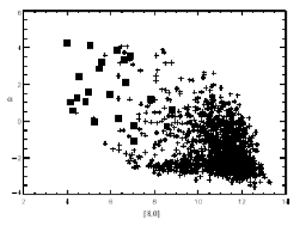
Figure 9: Plot of spectral index, $\alpha$, against source magnitude at 8.0 $\mu$m. The sources listed in Table LABEL:irs are marked with squares, while the remaining IRAC sources are marked with crosses.

We find little evidence for H₂ jets associated with the 8.0 $\mu$m “IRS” sources (see the Appendix for a detailed discussion), and only one of the four EROs has a definite H₂ jet. Most of the candidate jet sources in Table LABEL:sources are relatively faint at 8.0 $\mu$m, while $\sim$80% of the outflows listed in Table LABEL:jets have no obvious source identified at 8.0 $\mu$m. It thus seems clear that, with the exception of the massive DR21 and W75N outflows themselves, the H₂ jets are not driven by the massive protostars. Instead, low- or at most intermediate-mass YSOs seem to power each flow.

The candidate outflow sources are, however, very red (in comparison to the criteria used to select protostars from the Spitzer observations). Many will probably be Class 0 or early Class I sources. Some may be flat-spectrum or Class II YSOs viewed edge-on and therefore through their circumstellar disks, although if this were the case one would expect to see more Class II jet sources (with negative values of $\alpha$) viewed pole-on. It seems likely that many of the H₂ flows are powered by low-mass “protostars” that are too faint and/or too heavily embedded to be detected even by Spitzer.

Candidate central engines for the massive DR21 and W75N outflows remain elusive. Accurate Spitzer photometry of the IRS sources in each region is difficult, since at near- and mid-IR wavelengths these sources are often extended and bathed in diffuse emission. The brighter sources are also saturated at the longer wavelengths. In DR21, Smith et al. (2005) note that UCHii region DR21(D) is detected in the Spitzer bands and has an extremely red mid-IR SED. Even so, it is not well placed mid-way between the extensive H₂ flow lobes. Also, it does not coincide with the brightest dust-continuum peak in our 850 $\mu$m data. DR21(OH), on the other hand, is associated with a SCUBA core; it is also detected at mid-IR wavelengths, and again is extremely red. Its outflow is clearly traced in methanol maser emission (Plambeck & Menten, 1990; Kogan & Slysh, 1998, see also Fig. 12), though DR21(OH) itself is associated with multiple water masers (Forster et al., 1978; Mangum, Wooten & Mundy, 1992) and therefore probably comprises multiple sources, any one of which could drive the outflow.

The relationship between the infrared sources and multiple UCHii regions in W75N are discussed in detail by Shepherd, Kurtz & Testi (2004). The mid-IR properties of these sources are analysed by Persi, Tapia & Smith (2006). From their analysis of ground-based and Spitzer mid-IR photometry they propose that W75N-IRS 2 is a B3 star, while W75N-IRS 3 and W75N-IRS 4 are intermediate-mass Class II YSOs. In Fig. 5 W74N-IRS 1 is clearly elongated; here Persi, Tapia & Smith (2006) identify two sources, one coincident with the near-IR W75N-IRS 1 peak, and a second, much redder source coincident with the MM1 dust continuum peak (Shepherd, Testi & Stark, 2003) and VLA radio sources (Torrelles et al., 1997). This secondary mid-IR source is almost certainly associated with the W75N outflow source. Its position, RA(2000):20^h38^m36.5^s DEC(2000):42^∘37′33.6″is also notably coincident, to within an arcsecond, with the “W75N” 850 $\mu$m peak in Table. LABEL:scuba.

Overall, W75N and DR21 are similar in many ways. Both regions harbour a massive core containing clusters of Hii regions, some of which are ultra-compact. Both contain water, OH and methanol masers. Both are also associated with bright, near- and mid-IR nebulosity and clusters of tens of embedded sources, many of which are B-type (5–10  M_⊙) stars. Both are also surrounded by smaller, more compact clusters of just a few (or just one) early B-type stars plus associated low-mass stars. DR21 and W75N themselves drive very massive molecular outflows, which are almost parallel on the sky (as is the flow from DR21(OH)). And finally, numerous smaller-scale H₂ jets and outflows are found in the vicinity of each massive star-forming region, these jets being driven by low or at most intermediate-mass young stars.

4.2 General outflow characteristics: sizes, opening angles and orientations

Estimated jet parameters for the more prominent outflows are given in Table LABEL:jets. At a distance of 3 kpc a parsec-scale jet should be $>$70″ in length. At least five of the H₂ outflows meet this requirement. For a modest flow velocity of 100 km s^-1 a jet should reach a length in excess of a parsec in $\sim 10^{4}$ yrs; thus, a Class 0 source could easily be associated with a parsec-scale flow. Some of the long jets in Table LABEL:jets, like B 6-1:B 6-3 and C 8-1:C 8-5 do have candidate sources with SED slopes consistent with very red YSOs (Table LABEL:sources).

Precise jet opening angles ($\theta$) are rather difficult to measure, particularly at kilo-parsec distances. The emitting flanks of large-scale bow shocks are often much wider than the underlying jet (HH 212 is a spectacular example; Zinnecker, McCaughrean & Rayner, 1996), while changes in flow direction over time will increase the apparent flow opening angle. Moreover, if one includes all features along the flow axis, or just the extent of the leading bow shock, very different values can be inferred. Consequently, for a few flows in Table LABEL:jets we list a range of values; the smaller is measured between the candidate outflow source and the knot furthest from the source, while the larger value represents the maximum apparent flow opening angle that includes all emission features. If no YSO is identified, the angles are measured between the two most distant knots in the jet. Overall, the jets in the DR21 and W75N regions appear to have high degrees of collimation, consistent with the apparent youth of the candidate central engines in Table LABEL:sources.

Flow position angles on the sky are also listed in Table LABEL:jets. The two main DR21 and W75N outflows have almost the same position angle ($\sim$60^∘-70^∘). The DR21(OH) molecular outflow, which is not obviously traced in H₂, has a similar “east-west” position angle (Lai, Girart & Crutcher, 2003), as does the prominent H₂ jet B 6-1 to B 6-3. Each of these flows is orientated roughly orthogonal to the chain of 850 $\mu$m cores and the molecular ridge that runs north-south through DR21 towards W75N. If we simply count the number of flows in regions A and B (including the main DR21, DR21(OH) and W75N outflows) with position angles in the range 45^∘–135^∘  and compare this to the number of flows with angles in the range 0^∘–45^∘ and 135^∘–180^∘, we find a ratio of 11 to 6. (For the whole region imaged, the ratio is 25:10.) Moreover, a Kolmogorov-Smirnov test yields a probability of only 53% that the distribution of angles in areas A and B is homogeneously distributed between 0^∘ and 180^∘. It is therefore possible that the flow position angles are to some degree dictated by the large-scale cloud morphology. If the north-south elongation of the DR21/W75 ridge is produced by gravitational collapse along east-west orientated magnetic fields lines, then the random motions of individual star forming cores within the ridge are only moderately successful at scrambling the polar axes of the outflow sources. This process may be even less effective with the very massive YSOs, DR21, W75N, ERO 1 and DR21(OH), where the flows clearly are orthogonal to the north-south molecular ridge that extends through DR21. Note that Vallée & Fiege (2006) find that the magnetic field direction, inferred from 850 $\mu$m linear polarimetry observations, is orientated roughly orthogonal to the DR21 filament, as expected.

4.3 Spatial distribution of outflows and their relationship to YSO clustering

In busy star forming regions like DR21 and W75N, interactions between neighbouring stars as they pass by each other may inhibit disk formation, or even strip stars of their circumstellar disks. Since accretion drives outflows, YSOs without actively accreting disks will obviously not produce H₂ jets. In Figs. 11 to 15 one can see that clusters of YSOs do not generally coincide with an abundance of H₂ features. Although these areas are not entirely devoid of H₂ jets, H₂ features do seem to be more abundant in other regions, which show a paucity of YSOs (as identified by our Spitzer analysis), e.g. the region $\sim$1′ northwest of the western DR21 outflow lobe (Figs. 11 and 12) and 3′–5′ west of the busy L906E-IRS 3/IRS 4/IRS 5 cluster (Figs. 15). A stellar density plot is shown in Paper II.

To investigate this issue further, we consider whether outflow sources have fewer neighbours than YSOs with no obvious H₂ jet. To do this we count the number of neighbours each YSO has within a radius of 50 pixels (20″, or 0.3 pc). YSO neighbours are classified as Spitzer-identified protostars ($\alpha>0.25$) or pre-main-sequence stars ($0.25>\alpha>-1.60$), since all of these sources are likely to be in the same star forming regions and therefore potentially involved in star-star interactions or disk stripping. However, because all candidate outflow sources appear to possess reddened photospheres (e.g. Table LABEL:sources), we count neighbours only for the protostars. We have confined the analysis to a 8.0′$\times$10.7′ (1200$\times$1600 pixel) region centred near DR21-IRS 5, a 8.0′$\times$6.7′ region centred on W75N, and a 8.0′$\times$6.7′ region centred midway between L906E-IRS 3 and L906E-IRS 6. In other words, we focus only on regions where H₂ outflows are abundant (except for the region west of W75N, where we lack complete Spitzer data and therefore source classifications).

The resulting histograms are plotted in Fig. 10. The mean number of neighbours for candidate outflow sources is 1.4, while the mean for the remaining protostars is 1.8. Both values are, however, skewed by the large number of sources with no neighbours (the N$=$0 column in Fig. 10). Many of these sources lie on the periphery of the north-south DR 21 ridge, and around the edges of the W75N and L906E cores. If we exclude the sources with no neighbours from the statistics, then the outflow sources have a mean of 2.0 neighbours, while the remaining YSOs have a slightly higher mean of 2.9 neighbours. The latter is evident as a secondary peak in Fig. 10. The slight increase in the number of neighbours associated with non-outflow YSOs is an extremely tentative result, not only because of the modest number of sources considered, but also because of uncertainties in identifying outflow source candidates.

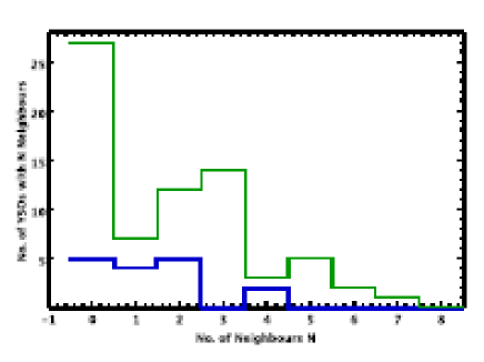
Figure 10: Plot of the number of YSO neighbours within a 50-pixel (20″) radius of protostars that are thought to drive outflows (thick/blue line) and those that have no obvious H₂ jets (thin/green line).

At first sight it seems that very few YSOs in the region drive detectable H₂ flows. By assuming that individual H₂ knots are parts of extended flows, we identify only 53 H₂ outflows in Table LABEL:jets, while our analysis of the Spitzer photometry reveals 165 protostars spread over the entire 0.8^∘ field. Some of the Class 0/I protostars will actually be pre-main-sequence Class II sources seen edge-on, and we do not include some of the very faintest knots and wisps of emission in Table LABEL:jets. Moreover, (1) the distance to DR 21 will limit our ability to detect some of the “weaker” flows, (2) extinction (approaching 100-200 magnitudes at V in the densest cores; Moore et al., 1991b; Chandler, Gear & Chini, 1993a; Persi, Tapia & Smith, 2006) will hide some H₂ features, and (3) east-west orientated outflows will probably break out of the denser cloud regions and therefore not be particularly bright in H₂ emission. Even so, we conclude that we have detected – within a factor of a few – roughly the same number of H₂ outflows as embedded protostars in DR21/W75.

4.4 Momentum injection and cloud support

Supersonic turbulent energy in giant molecular clouds is expected to decay on timescales of a few million years (Ostriker, Stone & Gammie, 2001). However, clouds last longer than this, harbouring multiple epochs of star formation at any one time. Outflows may be responsible for the continued injection of turbulent energy in to molecular clouds, maintaining virial equilibrium and thereby limiting cloud collapse and the overall star-formation efficiency.

The turbulent momentum (and energy) in a cloud is approximately equal to the product of the cloud mass and turbulent line width (and line width squared). The mass of the cores associated with DR21/W75 have been estimated from modeling of dust continuum observations (Moore et al., 1991a; Chandler, Gear & Chini, 1993a), molecular line maps (Dickel et al., 1978; Wilson & Mauersberger, 1990) and, more recently, as virial masses from extensive CS observations (Shirley et al., 2003). Core masses for DR21, DR21(OH) and W75N of between $1\times 10^{3}$  M_⊙ and $3\times 10^{4}$  M_⊙ are predicted. If we adopt a turbulent velocity of $\sim$3–5 km s^-1, estimated from sub-arminute-resolution maps in gas tracers that are optically thin and/or probes of high-density cores, like CS, NH₃ and C¹⁸O (e.g. Wilson & Mauersberger, 1990; Chandler et al., 1993b; Vallée & Fiege, 2006) – observations that are likely to yield velocities relatively unaffected by outflows or large-scale cloud motions – then a total momentum in the range $3\times 10^{3}$ – $1.5\times 10^{5}$  M_⊙  km s^-1 and turbulent energy in the range $1.8\times 10^{40}$ – $1.5\times 10^{42}$ J is inferred for each region.

The momentum and energy supplied by an outflow from a young star vary with time (e.g. Smith, 2000). Younger flows (from Class 0 sources) are more powerful than their Class I and Class II counterparts, and therefore provide a larger momentum flux, $P$, and energy flux (or mechanical power), $L$. Walawender, Bally & Reipurth (2005) note that one could use the canonical values for $P$ for Class 0 and Class I solar mass stars measured by Bontemps et al. (1996) to estimate the momentum supplied over the accreting lifetime of a young star. If $P({\rm Class~{}0})\sim 6\times 10^{-5}$  M_⊙ km s^-1 yr^-1 and $P({\rm Class~{}1})\sim 4\times 10^{-6}$  M_⊙ km s^-1 yr^-1, then assuming durations of $10^{4}$ and $10^{5}$ years for the Class 0 and Class I stages, over its lifetime an outflow from a low-mass protostar should inject $\sim$1.0  M_⊙ km s^-1 of momentum into its surroundings. The outflow kinetic energy scales with the velocity; since most of the molecular material in outflows is probably entrained in the relatively slow-moving wings of bow shocks (which explains why CO outflows are usually an order of magnitude slower than HH jets), then for a molecular flow velocity of $\sim$20 km s^-1, the kinetic energy supplied by a typical outflow would be $\sim 4\times 10^{37}$ J . The 50 or so flows from low-mass stars in DR21/W75 could therefore provide of the order of $\sim$50  M_⊙ km s^-1 of turbulent momentum and inject about 2$\times 10^{39}$ J of kinetic energy into the cloud over their lifetimes. Both values are less, by two to three orders of magnitude, than what is apparently needed to maintain the observed turbulent momentum and energy in the region. Note also that the trend toward east-west orientated outflows noted earlier, and the small filling factor of each collimated jet (with respect to the total volume of the cloud) limits the efficiency of momentum and energy transport to the global GMC environment.

But we have not considered the high-mass sources. Although these are relatively few in number, their outflows are more massive and more energetic, by three to four orders of magnitude. The momentum in the DR21 and W75N outflows, measured from CO observations, is of the order of $\sim 2\times 10^{4}$  M_⊙ km s^-1 and $10^{3}-10^{4}$  M_⊙ km s^-1, respectively (Garden et al., 1991b; Davis et al., 1998a; Shepherd, 2001). This would be more than enough to provide turbulent support against cloud collapse, if this momentum was distributed throughout the cloud. But of course these two flows do not impinge on the whole cloud; both are fairly well collimated and so probably efficiently “drill” through their molecular surroundings, rather than feed turbulence into the larger environment. Note that massive dense cores, traced at 850 $\mu$m, remain around DR21, DR21(OH) and W75N (Fig. 8); they are not entirely dispersed by the powerful outflows.

Finally, rather than use “mean” values for the momentum and energy of the outflows, we can infer these directly from the integrated H₂ line fluxes, since the outflow mechanical power should be directly related to the energy radiated in the entraining shock fronts. Davis & Smith (1996) point out that in strong-shock prompt entrainment scenarios, where the ambient gas is swept up in a momentum-conserving fashion to form the molecular “CO” outflow, the energy radiated in the wings of the entraining bow shock – the flux seen in H₂ and other coolants – should be equivalent to the mechanical power in the swept-up outflow. In regions A, B and C, the total H₂ 1-0S(1) line flux, $F_{\rm 1-0(S1)}$, measured from the H₂ flows identified in Table LABEL:jets (again not including the special case DR21 and W75N flows) is about $1\times 10^{-15}$ W m^-2. At a distance $d\sim$3 kpc, and assuming that the 1-0S(1) line represents 10% of all H₂ line radiation, then the total H₂ luminosity will be $L_{\rm H2}=10\times L_{\rm 1-0(S1)}\times 4\pi d^{2}=1\times 10^{27}$ W. Since there will be other important molecular coolants; H₂O, CO, etc. (Benedettini et al., 2000; Giannini, Nisini & Lorenzetti, 2002), the energy radiated in the outflow bow shocks will actually be 2-3 times higher. The observed line fluxes are also not corrected for extinction. The observed jets probably occupy regions of fairly modest extinction; an $A_{v}$ of 10 would boost the luminosity by a further factor of 2.5. The total radiated power is therefore probably an order of magnitude higher, $\sim 10^{28}$ W. For a dynamical age of $\sim 3\times 10^{11}$ sec (1 pc/100 km s^-1) the energy pumped into the cloud equates to $\sim 3\times 10^{39}$ J, which again seems to be insufficient to account for the turbulent energy in the GMC.

In conclusion, the current generation of low-mass YSO flows probably does not drive the observed cloud turbulence. However, many repeats of the current epoch of outflow activity, possible during the few million year timescale for turbulent decay in the GMC, might provide sufficient momentum and energy. Notably, the $10^{3}-10^{4}$ year outflow dynamical timescale is a factor of 10-100 times less than the turbulent decay time scale (for a $\sim$3 pc cloud and velocity of $\sim$3  km s^-1), as required. Imaging surveys of other high-mass star forming regions are required to establish whether the abundance of outflows in DR21/W75 is common in other regions, or whether DR21/W75 is uniquely active. The former would support the occurance of repeat epochs of outflow activity in this and other regions.

5 Summary and Conclusions

We compare near-IR and mid-IR images of the high-mass star forming regions DR21 and W75, obtained with the wide-field camera, WFCAM on the U.K. Infrared telescope, and the IRAC camera on the Spitzer Space telescope. 850 $\mu$m images of much of the region, obtained with the SCUBA bolometer array on the James Clerk Maxwell Telescope, are also considered.

The H₂ 1-0S(1) images obtained with WFCAM reveal numerous line-emission features, most of which appear to be associated with collimated flows. The Spitzer IRAC images were found to be of limited use in tracing these outflows, because of the intense PAH emission in the IRAC bands associated with background nebulosity, and because of limited spatial resolution in these very busy star-forming regions. However, the IRAC data were extremely useful for detecting YSOs, particularly massive, embedded sources, and for identifying potential outflow central engines. The near- and mid-IR photometry and stellar population are discussed in Paper II. The conclusions reached in this paper (Paper I) are described below.

1. The well-known W75N and DR21 high-mass star forming regions are surrounded by smaller clusters that harbour perhaps just one intermediate or high-mass star (the DR21-IRS and W75N-IRS sources). In the case of DR21, the SCUBA data reveal less evolved cores that are not generally associated with the “IRS-type” clusters, although these cores may eventually evolve into such clusters. The fact that the SCUBA cores are already distributed along the DR21 ridge suggests that the cores are dynamically distributed throughout the region before they evolve into intermediate or high-mass star forming clusters. As noted in Paper II, the more evolved YSO population traced by Spitzer is even more widely distributed.

2. Although we find a large number of H₂ emission-line features, many of which appear to be associated with collimated jets, these are usually not associated with either the young SCUBA cores or the compact infrared clusters noted above. Instead, they seem to be driven by independent protostars, probably low-mass Class 0/I sources distributed around the periphery of the dense 850 $\mu$m cores and north-south molecular ridge.

3. H₂ features associated with at least 50 individual outflows are identified. Many are knotty and well collimated, much like jets in nearby low mass star forming regions. At least five are parsec-scale flows. The orientations of the flows on the sky show some degree of order, with two thirds of the flows being roughly perpendicular (within a 90^∘ cone) to the north-south molecular ridge; we find only a 53% chance that the flows are randomly orientated.

4. We find very tentative evidence that clustering may inhibit disk accretion and thus the production of extensive outflows. We certainly do not see an enhancement in the number of outflows around compact clusters or groups of embedded protostars.

5. Although the low-mass YSO flows are abundant and widely distributed throughout the region, the observed outflow activity needs to be repeated 10-100 times if the flows are to provide sufficient momentum and kinetic energy to account for the turbulent motions in the large-scale molecular cloud. The current high-mass YSO flows associated with DR21 and W75N are sufficiently energetic. However, because these massive flows are well collimated, orientated orthogonal to the clumpy GMC that runs through DR21/W75, and because they are few in numbers, the transport of their momentum and energy to the ambient medium is probably relatively inefficient.

The mid-IR and far-IR observations very effectively trace the distribution of protostars and pre-stellar cores across the entire region. The narrow-band H₂ images complement these data by showing regions that are dynamically active, areas that may otherwise go unnoticed. Together, the UKIRT/WFCAM, Spitzer/IRAC and JCMT/SCUBA data yield a near-complete picture of star formation across the extensive region targeted here. Similar wide-field studies in the future at modest to high spatial resolutions – particularly with the advent of SCUBA-2 – should continue to improve our understanding of both low and high-mass star formation on global scales.

Appendix A Description of the H₂ jets

In Figs. 11 to 15 we show continuum-subtracted H₂ images of various regions along and adjacent to the DR21/W75 molecular ridge. We have separated the data into five areas for clarity, labeled A–E in Fig. 1. Individual H₂ knots, filaments and bow-shocks within each area have been numbered. Features that are thought to be part of the same outflow have been given consecutive numbers. For example, knots A 1-1, A 1-2 and A 1-3 are possibly part of the same jet in area A, while A 2-1, although still in area A, is probably part of a different flow. We also mark on each figure the locations of Spitzer sources with reddened photospheres; those with $\alpha>0.25$ are dubbed protostars, and those with $0.25>\alpha>-1.65$ we refer to as pre-main-sequence objects. Note that only sources detected in all four Spitzer IRAC bands were extracted from the data.

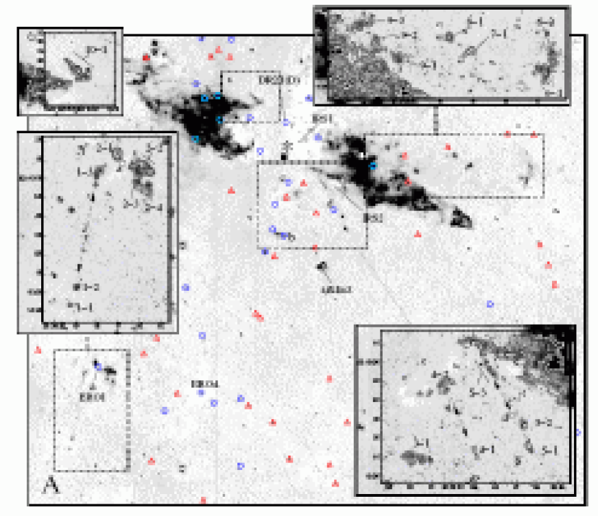
Figure 11: Continuum-subtracted H₂ 1-0S(1) image of region “A”, just to the south of DR21. Inset are contour-plots showing the prominent line-emission features in more detail. The micro-stepped data have been binned over 2x2 pixels to a scale of 0.4″ to improve the signal-to-noise on the extended H₂ features. Contour levels measure 0.4, 0.8, 1.6$\times 10^{-18}$ W m^-2 arcsec^-2 (black) and 3.2, 6.4, 12.8$\times 10^{-18}$ W m^-2 arcsec^-2 (white). The open circles mark the locations of the protostars ($\alpha>0.25$); the triangles mark the positions of the pre-main-sequence objects ($0.25>\alpha>-1.60$). Those that are possible jet sources are given reference letters and are also marked in the contour plots. The filled squares mark the positions of methanol masers in the DR21 outflow (Plambeck & Menten, 1990; Kogan & Slysh, 1998); the star indicates the location of the DR21 A-B-C Hii region (DR21 D is detected by Spitzer and is labeled).

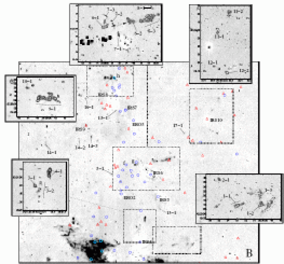
Figure 12: Continuum-subtracted H₂ 1-0S(1) image of region “B” just to the north of DR21. The positions of YSOs are again marked with open circles and triangles; possible jet sources are given letters. In the uppermost contour plot, methanol masers associated with the DR21(OH) outflow are marked with filled boxes (Plambeck & Menten, 1990; Kogan & Slysh, 1998), while water masers are marked with $\times$ symbols (Forster et al., 1978; Mangum, Wooten & Mundy, 1992). (See Fig.11 for further details.)

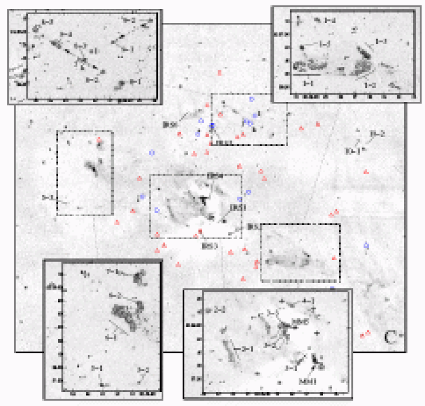
Figure 13: Continuum-subtracted H₂ 1-0S(1) image of region “C” centred on W75N (see Fig.11 for additional details). YSOs are again marked with open circles and triangles; possible jet sources are assigned letters. In the bottom-right contour plot the positions of water masers are marked with $\times$ symbols (Hunter et al., 1994; Torrelles et al., 1997); 2.7 mm continuum sources (Shepherd, Testi & Stark, 2003) are marked with pluses. Two of these mm sources, MM 1 and MM 5, coincide with W75N IRS1/W75N(B) and W75N IRS4/W75N(A), respectively.

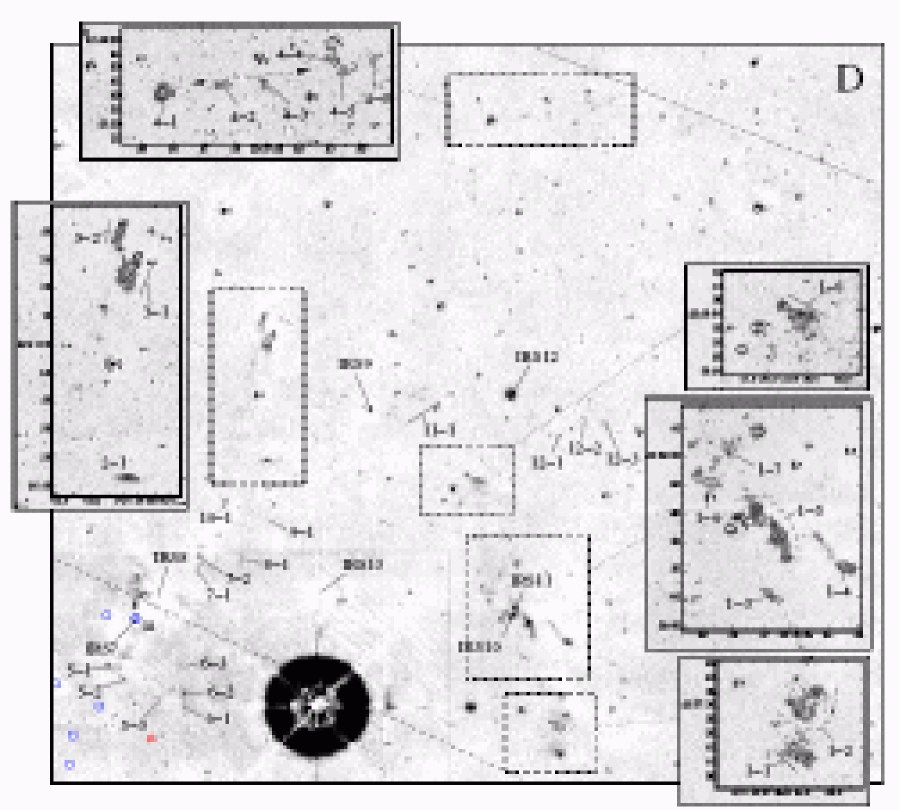
Figure 14: Continuum-subtracted H₂ 1-0S(1) image of region “D” $\sim$10′ to the west-north-west of W75N. YSO positions are again marked with circles and triangles, although the Spitzer data are incomplete in this region; the dashed line marks the edge of the 3.6 $\mu$m and 5.8 $\mu$m maps, while the dot-dashed line marks the edge of the 4.5 $\mu$m and 8.0 $\mu$m mosaics. (See Fig.11 for further details.)

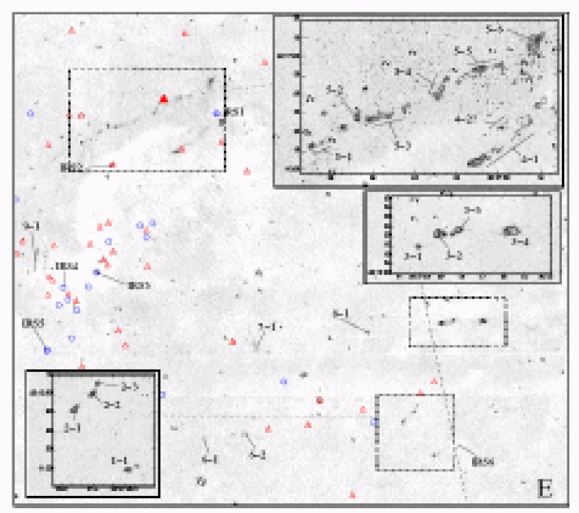
Figure 15: Continuum-subtracted H₂ 1-0S(1) image of L906E, region “E” (which is $\sim$20′ to the west of DR21). The positions of Spitzer YSO candidates are marked with circles and triangles; those that may drive the H₂ jets are given letters. The dashed line marks the approximate edge of the four Spitzer mosaics. (See Fig.11 for additional details.) The white thumb-print-like patch that coincides with L906E-IRS sources 1, 2 and 3 is an artifact from the subtracted K-band image. It was produced by patches of dirt on the WFCAM field lens (Dye et al., 2006).

A.1 DR21 south - region A

The area just to the south of DR 21 is shown in Fig. 11. The region includes the 850 $\mu$m core and mid-IR peak ERO 1, and the possible edge-on disk system ERO 4 discussed earlier. ERO 1 (star “a” in Table LABEL:sources) is identified as a reddened protostar in our analysis of the Spitzer IRAC data (it is marked with an open circle). Bright H₂ emission is associated with ERO 1, though not with ERO 4. Knots A 2-2, A 2-3 and A 2-4 outline a roughly conical structure with the apex facing ERO 1. This morphology could be indicative of a wide flow opening angle. The counter-flow is traced by knot A 2-1. The flow axis is clearly orientated roughly northeast-southwest.

A number of collimated H₂ jets are found scattered around the region. The jet described by A 1-1, A 1-2 and A 1-3 is almost certainly unrelated to ERO 1. This jet has no Spitzer-detected central engine (no open circle or triangle in Fig. 11). Nor is it associated with an 850 $\mu$m continuum peak.

Jet A 5-1 to A 5-3 and jet A 10-1 both point back roughly towards the infrared cluster associated with DR21 (DR21-IRS 1 in Fig. 2 and Fig. 11), and could therefore be driven by sources within this region. Alternatively, A 10-1 could be associated with the luminous, accreting infrared source and Hii region DR21 D (Smith et al., 2005), while knots A 5-1 and A 5-2 could be driven by the bright K-band source DR21-IRS 2 (Fig.2) or the reddened YSO “d” found midway between knots A 5-1 and A 5-3.

A 4-1 and A 4-2 possibly represent a faint jet and bow shock, with YSO “c” as a tentative source candidate. Notably, A 4-1:A 4-2 is parallel with A 5-1:A 5-3.

A 9-1, A 9-2 and A 9-3 may delineate another collimated flow that is roughly parallel with the main DR21 outflow, while knot A 6-1 may be a bow shock driven by a source to the southeast. Protostellar outflow source candidates are not found in the Spitzer data, however.

A 3-1 is a fairly bright though non-descript feature in the centre of the field. It is close to the Spitzer YSO star “b”, which is a protostar with a notably steep spectral index (Table LABEL:sources).

Additional faint knots and features are identified around the region which may or may not be associated with collimated flows. In many cases, the driving source of each flow is likely found along the molecular ridge that runs north-south through DR21 (Fig. 8).

A.2 DR21 north - region B

Area B (Fig. 12) is centred on DR21(OH) and the jet labeled B 6-1 to B 6-3. Orthogonal to this flow we detect a second, curving flow, knots B 7-1 to B 7-3. Neither flow seems to be associated with DR21(OH) itself: Lai, Girart & Crutcher (2003) and Vallée & Fiege (2006) both detect high-velocity CO emission associated with DR21(OH). However, the flow – mapped with a resolution of a few arcseconds by Lai, Girart & Crutcher (2003) – extends roughly east-west. Knot B 5-1 and possibly B 7-1 could be powered by this outflow.

Jet B 7-1 to B 7-3 could instead be driven by the bright, nebulous near-IR source $\sim$40″ to the west of DR21(OH), labeled DR21-IRS 6 in Fig.2. This source has Spitzer colours consistent with it being a reddened protostar, and is given reference letter “e” in Table LABEL:sources. Sources “f” or “g” may likewise be associated with jet B 6-1:B 6-3, although the pre-main-sequence YSO $\sim$10″ east of B 6-2 is also well placed. Stars “f” and “g” have particularly steep spectral indices. Comparison of our images with the NH₃ thermal emission maps of Mangum, Wooten & Mundy (1992) shows that these two jets lie roughly midway between (and to the west of) two compact clusters of cores (labeled MM 1/MM 2 and DR21(OH)N by this group). There is also no obvious dust clump associated with sources “f”, “g” or DR21-IRS 6/source “e”, or with either jet, in the 850 $\mu$m map in Fig. 8.

To the south in this figure we identify at least two (though possibly many more) collimated jets radiating outward from the DR21 core and IR cluster: feature B 1-1 is probably a jet driving the knotty bow B 1-2:B 1-3, while knot B 4-1 is a possible bow heading northward from DR21-IRS 4 or a source in the vicinity of DR21 itself. The compact knot B 3-1 and the fainter features labeled B 3-2 are enveloped in faint, diffuse emission. These may delineate further collimated flows extending northward from DR21. Including the jets identified in the previous section, we find at least five collimated jets radiating outward from the DR21 850 $\mu$m peak and cluster of Hii regions and embedded IR sources (six outflows if we include the main DR21 outflow itself).

Continuing northward along the molecular ridge, we find a chain of bright H₂ knots, B 9-1, which may be part of an east-west flow driven by the Spitzer YSO candidate source “h” at the western end of the B 9-1 chain. Alternatively, this feature may represent a fragmented bow shock in a flow driven by an embedded source to the south. Protostellar sources ERO 3, DR21-IRS 7 and DR21-IRS 8 are all possible candidates.

There are also faint knots $\sim$20″ south-east and $\sim$20″ north-east of DR21-IRS 10. Although this star is identified as a possible Class II or flat spectrum source in our Spitzer analysis (Table LABEL:irs), it is also associated with a discrete source at 850 $\mu$m (Fig. 8). Multiple unresolved sources may explain these seemingly contradictory data. IRS 10 certainly seems to be a strong source candidate for the collimated flow associated with B 11-1 and B 11-2.

There are other faint H₂ features distributed east of the ERO 3/FIR 1, FIR 2 and FIR 3 chain of dust cores, which we identify in the main panel in Fig. 12. These are also evident in Fig. 2. On morphological grounds alone, associating them with embedded sources along the molecular ridge is very difficult. Suffice to say that these features are generally within an arcminute ($\sim$0.9 pc) of the molecular ridge and may be part of east-west orientated jets.

A.3 W75N - region C

In Fig. 13 we show a continuum-subtracted H₂ image of W75N. The curving filaments of H₂ emission associated with the ends of the large-scale bipolar CO outflow, first identified by Davis et al. (1998a), are once again evident (features C 1-1 to C 1-4 and C 6-1:C 6-2). Torrelles et al. (1997) suggest that this large-scale flow could be driven by VLA 1, based on the elongated structure of this source at radio wavelengths. The source is well aligned with the apices of the proposed bow shocks C 1-1 to C 1-4 and C 6-1 and C 6-2. Alternatively, knot C 1-5, within the wings of the C 1-1 to C 1-4 bow, may be part of a collimated jet driving the bow shock, driven by the reddened K-band source W75N-IRS 2 (Fig. 3). Hydrogen recombination line emission has been detected from this star, so the source may be undergoing mass loss (Moore et al., 1991b). (The faint, diffuse emission a further arcminute to the south-west of knot C 1-2, noted by Shepherd, Testi & Stark (2003), is also evident in the main panel in Fig. 13, and as faint red features in Fig. 3.)

Knot C 7-1 to the north of the main W75N counterflow lies along the axis of the extended knot C 4-1 and may be part of the same flow. A Spitzer YSO candidate and three dust cores traced in 2.7 mm continuum emission (Shepherd, Testi & Stark, 2003) all lie on approximately the same axis (although the millimetre peaks have no bright K-band nor 8.0 $\mu$m counterparts). There are regions of diffuse H₂ emission between C 4-1 and C 7-1 (labeled NE-H and NE-I by Shepherd, Testi & Stark (2003)) which may also be part of this flow. Alternatively, this diffuse emission may be non-thermal, i.e. ambient gas fluorescently excited by neighbouring B stars.

A further $\sim$2′ to the north, knots C 8-1 to C 8-5 trace a very well collimated jet with almost the same position angle on the sky as the main W75N molecular outflow and the tentative C 4-1 to C 7-1 jet. However, if features C 9-1 and C 9-2 are also part of a collimated jet, this flow is almost orthogonal to the other outflows. Two Spitzer YSO sources “j” and “k” are candidates for C 8-1:C 8-5, while source “l” likely powers C 9-1:C 9-2. In our K-band image “k” and “l” are both slightly extended, their conical nebulae opening in the directions of the C 8-1:C 8-5 and C 9-1:C 9-2 jets respectively. All three protostars have steep spectral indices (Table LABEL:sources), and together these three stars are associated with a compact molecular core, labeled W75N-N in the 850 $\mu$m map in Fig. 8 (see also Table LABEL:scuba).

We also mention knots C 5-1 and C 5-2 on the southern edge of the main W75N outflow. These features form part of a very faint, narrow structure that snakes back toward W75N-IRS 3. However, one could also argue that C 5-1 and C 2-2 form part of a collimated jet, powered by source “i”, which notably coincides with SCUBA core W75N-E (Table LABEL:scuba; although this peak may actually trace CO line emission in SCUBA 850 $\mu$m filter bandpass, rather than dust continuum emission).

Subtraction of the diffuse continuum that envelopes W75N(A) and (B) reveals a number of elongated H₂ structures. These are thought to be bona fide line-emission features, since they are also recovered in the H₂ images of Davis et al. (1998a) and Shepherd, Testi & Stark (2003). The collimated structure C 2-1 and knot C 2-2 may be part of another collimated jet, although there is no bright K-band nor 8.0 $\mu$m source along this axis. Knots C 3-1 and C 3-3 may be bow shocks in the lobes of a bipolar jet, seen here as knotty feature C 3-2. Such a jet might be driven by a source midway between C 3-1 and C 3-3, although again no millimetre nor 8.0 $\mu$m peak is found here.

Shepherd and collaborators devote a series of papers to examining the properties of the sources in the central W75N cluster, and to identifying the source or sources that drive the large-scale CO outflow (Shepherd, 2001; Shepherd, Testi & Stark, 2003; Shepherd, Kurtz & Testi, 2004). They identify a possible complex of multiple, overlapping, small-scale outflows in W75N. They also point out that the VLA 1 jet lacks sufficient momentum to drive the large-scale CO outflow, and conclude that multiple sources may be producing the flow. Although our new near-IR images support the idea of multiple flows in W75N (and its immediate surroundings), the data do not really shed any further light on this issue.

A.4 W75N west - region D

Area D, to the west of W75N, was not observed in all four IRAC bands. Therefore, we can not use IRAC photometry to search for embedded YSOs. Even so, the region is of considerable interest. It includes a prominent bipolar molecular outflow labeled D 1-1 to D 1-8. On morphological grounds alone it seems likely that features D 1-1:D 1-2 and D 1-8 represent bow shocks at the ends of bipolar flow lobes. Midway between these features there is a compact cluster of at least three near-IR sources. Two targets, W75N-IRS 10 and 11, are also 8.0 $\mu$m point sources and are strong candidates for the outflow central engine (see also Fig. 5). W75N-IRS 11 in particular has a [4.5]-[8.0] colour of $\sim$3.1 (Table LABEL:irs) and is coincident with H₂ emission.

The elongated H₂ “fingers” D 3-1 and D 3-2 in Fig. 14 are reminiscent of the “bullets” in Orion (and perhaps knot B 4-1). These may originate from the bright K-band/8.0 $\mu$m sources W75N-IRS 7 (source “m”) or W75N-IRS 8. The latter was only observed in two IRAC bands, though like W75N-IRS 7 it is quite red (Table LABEL:irs).

Further to the north, the H₂ features D 4-1 to D 4-6 again describe a collimated jet. Features D 4-4 and D 4-5 are probably the wings of – and D 4-6 the cap of – a westward-moving bow shock.

In Fig. 3 and 5 we label four other interesting K-band/8.0 $\mu$m sources, W75N-IRS 9, 12, 13 and 14. There is very faint H₂ emission between sources W75N-IRS 9 and 12, labeled D 11-1 in Fig. 14. Additional faint H₂ jets and knots are detected west of W75N-IRS 12 and around W75N-IRS 7/IRS 8. Sources 13 and 14 appear to be point sources within small ionised shells which we see clearly in Fig. 3 in scattered light and/or recombination-line emission. There is possibly some fluorescent H₂ emission along the edges of each shell. We see no evidence for H₂ jets associated with either source, however.

A.5 L906E - region E

Finally, to the west of DR21 there is a cluster of nebulous embedded sources and a bok-globule-like region of increased extinction in the near-IR. These features lie on the eastern edge of the Lynds dark cloud L906. Unfortunately this area is outside the field of view of the SCUBA 850 $\mu$m map, and it was not discussed in great detail by Marston et al. (2004). However, in Fig. 6 and Fig. 15 one easily sees the rich nature of this region.

We clearly identify a number of collimated jets in area E. The wishbone-shaped feature E 4-1, E 4-2 and E 5-1 to 5-6 is associated with a bright 8 $\mu$m peak and spherical core of mid-IR emission, which we dub L906E-IRS 1. This source has a particularly steep spectral index and certainly qualifies as an ERO (Table LABEL:sources). Even so, the H₂ knots are probably associated with independent flows, rather than a single wide-angled wind.

The H₂ features E 3-1 to E 3-4 are unfortunately beyond the edges of all four of the Spitzer IRAC images, so these cannot be used to search for the possible outflow source. However, they likely form part of a knotty jet. So might E 2-1 to E 2-3, which lie 20″–40″ to the southeast of a pair of Class II/flat spectrum sources.

The faint knots E 6-1 and E 6-2 likely trace yet another collimated flow, while feature E 7-1 appears to be a faint bow shock, possible driven by a source in the vicinity of L906E-IRS 3.

Of the remaining H₂ feature, E 1-1 is close to a nebulous K-band source L906E-IRS 6 (situated $\sim$25′ to the west-northwest of E 1-1). This source was just inside the 5.8 $\mu$m and 8.0 $\mu$m Spitzer field of view, and again appears to be fairly red (Table LABEL:irs).

References

- André, Ward-Thompson & Barsony (1993) André P., Ward-Thompson D., Barsony M, ApJ, 406, 122
- Allen et al. (2004) Allen L.E. et al., 2004, ApJS, 154, 363
- Baart et al. (1986) Baart E.E., Cohen R.J., Davies R.D., Norris R.P., Rowland P.R., 1986, MNRAS, 219, 145
- Benedettini et al. (2000) Benedettini M., et al., 2000, A&A, 359, 148
- Bontemps et al. (1996) Bontemps S., Andre P., Tereby S., Cabrit S., 1996, A&A, 311, 858
- Casali et al. (2006) Casali M., et al., 2006, in prep.
- Chandler, Gear & Chini (1993a) Chandler C.J., Gear W.K., Chini R., 1993a, MNRAS, 260, 337
- Chandler et al. (1993b) Chandler C.J., Moore T.J.T., Mountain C.M., Yamashita T., 1993b, MNRAS, 261, 694
- Cyganowski et al. (2003) Cyganowski C.J., Reid M.J., Fish V.L., Ho P.T.P., 2003, ApJ, 596, 344
- Davis et al. (1998a) Davis C.J., Moriarty-Schieven G.H., Eislöffel J., Hoare M.G., Ray T.P., 1998a, AJ, 115, 1118
- Davis & Smith (1996) Davis C.J., Smith M.D., 1996, A&A, 310, 961
- Davis, Smith & Moriarty-Schieven (1998b) Davis C.J., Smith M.D., Moriarty-Schieven G.H., 1998b, MNRAS 299, 826
- Dickel et al. (1978) Dickel J.R., Dickel H.R., Wilson W.J., 1978, 223, 840
- Dickel et al. (1986) Dickel H.R., Goss W.M., Rots A.H., Blount H.M., 1986, A&A, 162, 221
- van Dishoeck (2004) van Dishoeck E.F., 2004, ARA&A, 42, 119
- Downes & Rinehart (1966) Downes D., Rinehart R., 1966, ApJ, 144, 937
- Dye et al. (2006) Dye S., et al., 2006, MNRAS, in press
- Fazio et al. (2004) Fazio G.G., et al., 2004 ApJS, 154, 10
- Fernandez, Brand & Burton (1997) Fernandez A.F.L., Brand P.W.J.L., Burton M.G., 1997, MNRAS, 290, 216
- Fischer et al. (1985) Fischer J., Sanders D.B., Simon M., Solomon P.M., 1985, ApJ, 293, 508
- Forster et al. (1978) Forster J.R., Welch W.J., Wright M.C.H., Baudry A., 1978, ApJ, 221, 137
- Garden & Carlstrom (1992) Garden R.P., Carlstrom J.E., 1992, ApJ, 392, 602
- Garden et al. (1991a) Garden, R.P., Geballe, T.R. Gatley, I., Nadeau, D. 1991a, ApJ, 366, 474
- Garden et al. (1991b) Garden R.P., Hayashi M., Gatley I., Hasegawa T., Kaifu N., 1991b, ApJ, 374, 540
- Genzel & Downes (1977) Genzel R., Downes D., 1977, A&AS, 30, 145
- Giannini, Nisini & Lorenzetti (2002) Giannini T., Nisini B., Lorenzetti D., 2002, ApJ, 555, 40
- Gibb et al. (2007) Gibb A.G., et al., 2007, in prep.
- Gibb et al. (2000) Gibb E.L., et al., 2000, ApJ, 536, 347
- Harris (1973) Harris S., 1973, MNRAS, 162, 5
- Haschick et al. (1981) Haschick A.D., Reid M.J., Burke B.F., Moran J.M., Miller G., 1981, ApJ, 244, 76
- Hewett et al. (2006) Hewett P.C., Warren S.J., Leggett S.K., Hodgkin S.T., 2006, MNRAS, in press
- Holland et al. (1999) Holland W.S., et al. 1999, MNRAS, 303, 659
- Hunter et al. (1994) Hunter T.R., Taylor G.B., Felli M., Tofani G., 1994, A&A, 284, 215
- Hutawarakorn, Cohen & Brebner (2002) Hutawarakorn B., Cohen R.J., Brebner G.C., 2002, MNRAS, 330, 349
- Irwin et al. (2006) Irwin M., et al., 2006 in prep.
- Jenness, Lightfoot & Holland (1998) Jenness T., Lightfoot J.F., Holland W.S., 1998, in Advanced Technology MMW, radio and teraherz telescopes, Phillips T. eds, Proc SPIE, 3357, 638
- Joshi (2005) Joshi Y.C., 2005, MNRAS, 362, 1259
- Kogan & Slysh (1998) Kogan L., Slysh V., 1998, ApJ, 497, 800
- Kumar et al. (2006) Kumar M.S.N, Davis C.J., Grave J.M.C., Ferreira B., Froebrich D., 2007, MNRAS, submitted. (Paper II)
- Lada (1987) Lada C.J., 1987 in IAU Symp. 115, Star Formation Regiopns, eds. M. Peimbert, J. Jugaku (Dordrecht: Reidel), p.1.
- Lada et al. (2006) Lada C.J. et al., 2006, AJ, 131, 1574
- Lai, Girart & Crutcher (2003) Lai S.-P., Girart J.M., Crutcher R.M., 2003, ApJ, 598, 392
- Liechti & Walmsley (1997) Liechti S., Walmsley C.M., 1997, A&A, 321, 625
- Mangum, Wooten & Mundy (1991) Mangum J.G., Wooten A., Mundy L.G., 1991, ApJ, 378, 576
- Mangum, Wooten & Mundy (1992) Mangum J.G., Wooten A., Mundy L.G., 1992, ApJ, 388, 467
- Marston et al. (2004) Marston A.P. et al., 2004, ApJS, 154, 333.
- Megeath et al. (2004) Megeath S.T. et al., 2004, ApJS, 154, 367
- Moore et al. (1991a) Moore T.J.T., Mountain C.M., Yamashita T., 1991a, MNRAS, 248, 79
- Moore et al. (1991b) Moore T.J.T., Mountain C.M., Yamashita T., McLean I.S., 1991b, MNRAS, 248, 377
- Noriega-Crespo et al. (2004) Noriega-Crespo A., Moro-Martin A., Carey S., Morris P.W., Padgett D.L., Latter W.B., Muzerolle J., 2004, ApJS, 154, 402
- Odenwald & Schwartz (1993) Odenwald S.F., Schwartz P.R., 1993, ApJ, 405, 706
- Ostriker, Stone & Gammie (2001) Ostriker E.C., Stone J.M., Gammie C.F., 2001, ApJ, 546, 980
- Persi, Tapia & Smith (2006) Persi P., Tapia M., Smith H.A., 2006, A&A, 445, 971
- Plambeck & Menten (1990) Plambeck R.L., Menten K.M., 1990, ApJ, 364, 555
- Roelfsema, Goss & Geballe (1989) Roelfsema P.R., Goss W.M., Geballe T.R., 1989, A&A, 222, 247
- Sandell, Jessop & Jenness (2001) Sandell G., Jessop N., Jenness T., 2001, The SCUBA Map Reduction Cookbook, Starlink Cookbook 11.2 (Oxon: CCLRC), www.starlink.rl.ac.uk/star/docs/sc11.htx/sc11.html
- Sault, Teuben & Wright (1995) Sault R.J., Teuben P.J., Wright M.C.H., 1995, in ASP Conf. Ser. 77: Astronomical Data Analysis Software and Systems IV, eds. R.A. Shaw, H.E. Payne, and J.J.E. Hayes (Astronomical Society of the Pacific: San Francisco), p.433
- Schneider et al. (2006) Schneider N., Bontemps S., Simon R., Jakob H., Motte F., Miller M., Kramer C., StutzkiJ., 2006, A&A, in press
- Shepherd (2001) Shepherd D.S., 2001, ApJ, 546, 345
- Shepherd, Testi & Stark (2003) Shepherd D.S., Testi L., Stark D.P., 2003, ApJ, 584, 882
- Shepherd, Kurtz & Testi (2004) Shepherd D.S., Kurtz S.E., Testi L., 2004, ApJ, 601, 952
- Shirley et al. (2003) Shirley Y.L., Evans N.J., Young K.E., Knez C., Jaffe D.T., 2003, ApJS, 149, 375
- Smith et al. (2005) Smith H.A., et al., 2005, In: Proceedings of the dusty and molecular universe: a prelude to Herschel and ALMA, ed. A. Wilson, ESA SP-577, ESA Publications Division, p.197
- Smith et al. (2006) Smith H.A., Hora J.L., Marengo M., Pipher J.L., 2006, ApJ, in press
- Smith (2000) Smith M.D., 2000, Irish Astron. J., 27, 25
- Smith, Eislöffel & Davis (1998) Smith M.D., Eislöffel J., Davis C.J., 1998, A&A 327, 1206
- Smith & Rosen (2005) Smith M.D., Rosen A., 2005, MNRAS, 357, 1370
- Torrelles et al. (1997) Torrelles J.M., Gomez J.F., Rodriguez L.F., Ho P.T.P., Curiel, S., Vazquez R., 1997, 489, 744
- Vallée & Fiege (2006) Vallée J.P., Fiege J.D., 2006, ApJ, 636, 332
- Walawender, Bally & Reipurth (2005) Walawender J., Bally J., Reipurth B., 2005, AJ, 129, 2308
- Westerhout (1958) Westerhout G., 1958, Bull. Astron. Institutes of the Netherlands, 14, 215
- Wilson & Mauersberger (1990) Wilson T.L., Mauersberger R., 1990, A&A, 239, 305
- Zinnecker, McCaughrean & Rayner (1996) Zinnecker H., McCaughrean M.J., Rayner J., 1996, Nature, 465, 236