Virialization of cosmological structures in models with time varying equation of state

Abstract

We study the virialization of the cosmic structures in the framework of flat cosmological models where the dark energy component plays an important role in the global dynamics of the universe. In particular, our analysis focuses on the study of the spherical matter perturbations, as the latter decouple from the background expansion and start to “turn around” and finally collapse. We generalize this procedure taking into account models with an equation of state which vary with time, and provide a complete formulation of the cluster virialization attempting to address the nonlinear regime of structure formation. In particular, assuming that clusters have collapsed prior to the epoch of $z_{\rm f}\simeq 1.4$, in which the most distant cluster has been found, we show that the behavior of the spherical collapse model depends on the functional form of the equation of state.

Keywords: clusters: formation- cosmology:theory - large-scale structure of universe

1 Introduction

It is well known that the available high quality cosmological data (Type Ia supernovae, CMB, etc.) are well fitted by an emerging “standard model”, which contains cold dark matter (CDM) to explain clustering and an extra component with negative pressure, the dark energy, to explain the observed accelerated cosmic expansion. The last decades there have been many theoretical speculations regarding the nature of the above exotic dark energy. Most of the authors claim that a scalar field which rolls down the potential $V(\phi)$ (Ratra & Peebles 1988; Caldwell, Dave, Steinhardt 1998; Peebles & Ratra 2003) could resembles that of the dark energy. The cosmic equation of state is given by $p_{Q}=w\rho_{Q}$, where $p_{Q}$ is the pressure and $\rho_{Q}$ is the corresponding density of the dark energy. Owing to the fact that $w<-1/3$ is related to the potential of the dark energy field, having an indication about its value may help us to understand the nature of the dark energy.

However, a serious issue here is how the large scale structures and in particular galaxy clusters form. The cluster distribution traces basically scales that have not yet undergone the non-linear phase of gravitationally clustering, thus simplifying their connections to the initial conditions of cosmic structure formation. The so called spherical collapse model, which has a long history in cosmology, is a simple but still a fundamental tool to describe the growth of bound systems in the universe via gravitation instability (Gunn & Gott 1972). In the last decade many authors have been involved in this kind of studies and have found that the main parameters of the spherical collapse model such as the ratio between the final and the turn around radius (hereafter collapse factor), is affected by the dark energy (Lahav et al. 1991; Wang & Steinhardt 1998; Iliev & Shapiro 2001; Battye & Weller 2003; Basilakos 2003; Weinberg & Kamionkowski 2003; Mota & van de Bruck 2004; Horellou & Berge 2005; Zeng & Gao 2005; Maor & Lahav 2005; Percival 2005; Wang 2006; Nunes & Mota 2006).

The aim of this work is along the same lines, attempting to investigate the cluster formation processes by generalizing the non-linear spherical model for a family of cosmological models with an equation of state parameter being a function of time, $w=w(t)$. This can help us to understand better the theoretical expectations of negative pressure models as well as the variants from the Quintessence ($w=w_{0}=const$ with $-1\leq w_{0}<-1/3$) and Phantom ($w=w_{0}=const$ with $w_{0}<-1$) case respectively.

The structure of the paper is as follows. The basic elements of the cosmological equations are presented in section 2. Sections 3 and 4 outline the spherical collapse analysis in models where $w$ is a function of time and finally, we draw our conclusions in section 5.

2 The basic Cosmological Equations

For homogeneous and isotropic cosmologies, driven by non relativistic matter and an exotic fluid with equation of state, $p_{Q}=w(\alpha)\rho_{Q}$ with $p_{Q}<0$, the Einstein field equations can be given by:

$$\left(\frac{\dot{\alpha}}{\alpha}\right)^{2}=\frac{8\pi G}{3}(\rho_{\rm m}+\rho_{Q})-\frac{k}{\alpha^{2}}$$ (1)

with $k=-1,0$ or 1 for open, flat and closed universe respectively and

$$\frac{\ddot{\alpha}}{\alpha}=-4\pi G\left[\left(w(\alpha)+\frac{1}{3}\right)\rho_{Q}+\frac{1}{3}\rho_{\rm m}\right]\;\;,$$ (2)

where $\alpha(t)$ is the scale factor, $\rho_{\rm m}=\rho_{\rm m0}\alpha^{-3}$ is the background matter density and $\rho_{Q}=\rho_{Q0}f(\alpha)$ is the dark energy density, with:

$$f(\alpha)={\rm exp}\left[3\int_{\alpha}^{1}\left(\frac{1+w(u)}{u}\right){\rm d}u\right]\;\;.$$ (3)

Thus, the scale factor evolves according to Friedmann equation: $H^{2}\equiv(\dot{\alpha}/\alpha)^{2}$. The relation between the time and the scale factor is given by

$$\frac{dt}{d\alpha}=\frac{1}{H(\alpha)\alpha}\;\;,$$ (4)

where the Hubble parameter is written: $H(\alpha)=H_{0}E(\alpha)$ and $H_{0}$ is the Hubble constant with

$$E(\alpha)=\left[\Omega_{\rm m}\alpha^{-3}+\Omega_{k}\alpha^{-2}+\Omega_{Q}f(\alpha)\right]^{1/2}\;\;\;,$$ (5)

while $\Omega_{\rm m}=8\pi G\rho_{\rm m0}/3H_{0}^{2}$ (density parameter), $\Omega_{k}=-k/H_{0}$ (curvature parameter), $\Omega_{Q}=8\pi G\rho_{Q0}/3H_{0}^{2}$ (dark energy parameter) at the present time with $\Omega_{\rm m}+\Omega_{k}+\Omega_{Q}=1$.

In addition, to $\Omega_{m}(\alpha)$ also $\Omega_{Q}(\alpha)$ could evolve with the scale factor as

$$\Omega_{\rm m}(\alpha)=\frac{\Omega_{\rm m}\alpha^{-3}}{E^{2}(\alpha)}\;\;\;{\rm and}\;\;\;\Omega_{Q}(\alpha)=\frac{\Omega_{Q}f(\alpha)}{E^{2}(\alpha)}\;\;.$$ (6)

Note that in this paper we consider a spatially flat ($k=0$) low-$\Omega_{\rm m}=0.3$ cosmology with $H_{0}=72$ Km s^-1Mpc^-1 which is in agreement with the cosmological parameters found from the recent observations (see Freedman et al. 2001; Spergel et al. 2003; Tegmark et al. 2004; Basilakos & Plionis 2005; Spergel et al. 2006 and references therein). Finally, in order to address the negative pressure term it is essential to define the functional form of the equation parameter $w=w(\alpha)$ [see section 4].

3 Virialization in the Spherical Model

The spherical collapse model is still a powerful tool, despite its simplicity, for understanding how a small spherical patch of homogeneous overdensity forms a bound system via gravitation instability. Technically speaking, the basic cosmological equations, mentioned before, are valid either for the entire universe or for homogeneous spherical perturbations [by replacing the scale factor with radius $R(t)$]

$$\frac{\ddot{R}}{R}=-4\pi G\left[\left(w(R)+\frac{1}{3}\right)\rho_{\rm Qc}+\frac{1}{3}\rho_{\rm mc}\right]\;\;,$$ (7)

where $\rho_{\rm mc}$ and $\rho_{\rm Qc}$ is the time-varying matter and dark energy density respectively (for spherical perturbations).

We study the cluster virialization in models with dark energy, generalizing the notations of Lahav et al. (1991), Wang & Steinhardt (1998), Mainini et al. (2003); Basilakos (2003), Lokas (2003) Mota & van de Bruck (2004), Horellou & Berge (2005), Zeng & Gao (2005), Maor & Lahav (2005), Bartelmann, Doran & Wetterich (2005), Nunes & Mota (2006) and Wang (2006) in order to take into account models with a time varying equation of state. Thus, in this section, we review only some basic concepts of the problem. Within the framework of the spherical collapse model we assume a spherical mass overdensity shell, utilizing both the virial theorem $T_{c}=-\frac{1}{2}U_{Gc}+U_{Qc}$ and the energy conservation $T_{c,f}+U_{Gc,f}+U_{Qc,f}=U_{Gc,t}+U_{Qc,t}$ where, $T_{c}$ is the kinetic energy, $U_{Gc}=-3GM^{2}/5R$ is the potential energy and $U_{Qc}$ is the potential energy associated with the dark energy for the spherical overdensity. In particular, the potential energy induced by the dark energy component (see Horellou & Berge 2005 and references therein) is

$$U_{Qc}=(1+3w)\rho_{Qc}\frac{4\pi GM}{10}R^{2}\;\;\;.$$ (8)

Using the above formulation we can obtain a cubic equation which relates the ratio between the final (virial) $R_{\rm f}$ and the turn-around outer radius $R_{\rm t}$:

$$2n_{1}\lambda^{3}-(2+n_{2})\lambda+1=0$$ (9)

where $\lambda=\frac{R_{\rm f}}{R_{\rm t}}$ is the collapse factor,

$$n_{1}=-(3w+1)\frac{\Omega_{Q}f(\alpha_{\rm f})}{\zeta\Omega_{\rm m}\alpha_{\rm t}^{-3}}$$ (10)

and

$$n_{2}=-(3w+1)\frac{\Omega_{Q}f(\alpha_{\rm t})}{\zeta\Omega_{\rm m}\alpha_{\rm t}^{-3}}$$ (11)

with

$$\zeta\equiv\frac{\rho_{\rm mc,t}}{\rho_{\rm m,t}}=\left(\frac{R_{\rm t}}{\alpha_{\rm t}}\right)^{-3}$$ (12)

(the definition of the $\alpha_{\rm t}$ and $\alpha_{\rm f}$ factors are presented bellow).

However, we would like to point out that there is some confusion in the literature regarding eq.(9) which is based on energy conservation. Indeed recently it has been shown (Maor & Lahav 2005) that the above formulation is problematic due to the fact that the total energy of the bound system is not conserved in dark energy models with $w\neq-1$. In order to avoid these systematic effects in this work we utilize two different assumptions. First of all, we assume that when the matter epoch just begins, the dark energy moves synchronously with ordinary matter on both, the Hubble scale and the galaxy cluster scale, the so called clustered dark energy scenario (see Zeng & Gao 2005 and references therein). It is interesting to mention that the synchronous dark energy evolution (hereafter clustered) was designed to conserve energy. In particular, Maor & Lahav (2005) address the issue of the clustered dark energy model based on the following assumptions: (i) clustered quintessence considering that the whole system virializes (matter and dark energy) and (ii) the dark energy remains clustered but now only the matter virializes (for more details see their section 4). Note, that in this work we are utilizing the second possibility. In that case the equation which defines the collapse factor becomes:

$$(1+q)\lambda-\frac{q}{2}(1-3w)\lambda^{-3w}=\frac{1}{2}$$ (13)

where the factor $q$ is given by

$$q=\frac{\rho_{\rm Q,t}}{\rho_{\rm mc,t}}=\frac{\rho_{\rm Q,t}}{\zeta\rho_{\rm m,t}}=\frac{\nu}{\zeta}$$ (14)

(the definition of the $\nu$ parameter is presented in section 3.1).

If we assume that the dark energy component in a galaxy cluster scale can be treated as being homogeneous then we get the following cubic equation defined by Maor & Lahav (2005)

$$2q\lambda^{3}-(1+q)\lambda+\frac{1}{2}=0\;\;,$$ (15)

Although it was pointed out recently (see Wang 2006) that if the value of $q$ is less than 0.01 then the problem of energy conservation does not really affect the virialization process and thus eq.(9) is still a good approximation.

From now on, we will call $\alpha_{\rm t}$ the scale factor of the universe where the overdensity reaches at its maximum expansion and $\alpha_{\rm f}$ the scale factor in which the sphere virializes, while $R_{\rm t}$ and $R_{\rm f}$ the corresponding radii of the spherical overdensity. Note that $\rho_{\rm mc,t}$ is the matter density which contains the spherical overdensity at the turn around time while $\rho_{\rm m,t}$ is the background matter density at the same epoch. Therefore, for bound perturbations which do not expand forever, the time needed to re-collapse is twice the turn-around time, $t_{\rm f}=2t_{\rm t}$. Doing so and taking into account eq.(4), it is easy to estimate the relation between the $\alpha_{\rm f}$ and $\alpha_{\rm t}$

$$\int_{0}^{\alpha_{\rm f}}\frac{1}{H(\alpha)\alpha}{\rm d}\alpha=2\int_{0}^{\alpha_{\rm t}}\frac{1}{H(\alpha)\alpha}{\rm d}\alpha\;\;.$$ (16)

In order to reduce the parameter space of the overall problem we put further observational constrains. Indeed, $\alpha_{\rm f}$ can be defined from the literature assuming that clusters have collapsed prior to the epoch of $z_{\rm f}\simeq 1.4$ in which the most distant cluster has been found (Mullis et al. 2005; Stanford et al. 2006). Therefore, considering $\alpha_{\rm f}\simeq 0.41$ and utilizing eq.(16), it is routine to obtain the scale factor at the turn around time. In the case of a $\Lambda$ cosmology we get an analytical solution:

$${\rm sin^{-1}h}\left(a_{\rm f}^{3/2}\sqrt{\nu_{0}}\right)=2{\rm sin^{-1}h}\left(a_{\rm t}^{3/2}\sqrt{\nu_{0}}\right)$$ (17)

where $\nu_{0}=(1-\Omega_{\rm m})/\Omega_{\rm m}$. While for the general problem we have to solve equation (16) numerically. The ratio between the scale factors converges to the Einstein de Sitter value $\left(\frac{\alpha_{\rm f}}{\alpha_{\rm t}}\right)=2^{2/3}$ at high redshifts.

3.1 The rescaled equations

In this section we present some of the basic concepts of the spherical collapse model. In particular, we assume a spherical overdensity which contains a dark energy component which behaves either as clustered or homogeneous. For a flat cosmology ($k=0$), using the basic differential equations (see eq.1 and 7) and performing the following transformations

$$x=\frac{\alpha}{\alpha_{\rm t}}\;\;\;\;{\rm and}\;\;\;\;y=\frac{R}{R_{\rm t}}\;\;\;,$$ (18)

the evolution of the scale factors of the background and of the perturbation are governed respectively by the following two equations:

$${\dot{x}}^{2}=H_{\rm t}^{2}\Omega_{\rm m,t}\left[\Omega_{\rm m}(x)x\right]^{-1}$$ (19)

and

$${\ddot{y}}=-\frac{H_{\rm t}^{2}\Omega_{\rm m,t}}{2}\left[\frac{\zeta}{y^{2}}+\nu yI(x,y)\right]\;\;\;.$$ (20)

Note, that in order to obtain the above set of equations we have used the following relations:

$$\rho_{\rm mc}=\rho_{\rm mc,t}\left(\frac{R}{R_{\rm t}}\right)^{-3}=\frac{\zeta\rho_{\rm m,t}}{y^{3}}$$ (21)

and

$$I(x,y)=\left\{\begin{array}[]{cc}\left[1+3w(R(y))\right]\frac{f(R(y))}{f(\alpha_{\rm t})}&\mbox{Clustered DE}\\ \left[1+3w(x)\right]f(x)&\mbox{Homogeneous DE}\end{array}\right.$$ (22)

with

$$\nu=\frac{\rho_{\rm Q,t}}{\rho_{\rm m,t}}=\frac{1-\Omega_{\rm m,t}}{\Omega_{\rm m,t}}\;\;\;.$$ (23)

The function $R(y)$ is given by the combination of eq.(12) and eq.(18): $R(y)=R_{\rm t}y=\zeta^{-1/3}\alpha_{\rm t}y$. Finally, $\Omega_{\rm m}(x)$ is given by

$$\Omega_{\rm m}(x)=\frac{1}{1+\nu x^{3}f(x)}\;\;.$$ (24)

3.2 The general solution for the clustered dark energy scenario

In this section we present our analytical solution of the $\zeta$ parameter by integrating the above system of differential equations, (eq.19 and eq.20), using at the same time the boundary conditions of $({\rm d}y/{\rm d}x)_{x=1}=0$ and $y=1$. In the case of a homogeneous dark energy the above system is solved only numerically. The novelty of our approach here is that for the clustered dark energy case the system can be solved analytically including models, where the dark energy parameter $w$ is a function of the cosmic time. Indeed, due to the fact that now the second part of eq.(20) is a function only of $y$ we can perform easily the integration

$${\dot{y}}^{2}=-H_{\rm t}^{2}\Omega_{\rm m,t}\left[-\zeta y^{-1}+G(y)-C\right]$$ (25)

where $C$ is the integration constant and

$$G(y)=\frac{\nu}{f(\alpha_{\rm t})}\int y\left[1+3w(R(y))\right]f(R(y)){\rm d}y\;\;.$$

Considering now that the functional form of $f(R(y))$ is exponential (see the appendix) we have the following useful formula:

$$\begin{array}[]{rcl}\int y[1+3w(R(y))]f(R(y)){\rm d}y=-2\int yf(R(y)){\rm d}y\\ -\int y^{2}\frac{{\rm d}f(R(y))}{{\rm d}y}{\rm d}y=-y^{2}f(R(y))\;\;\;.\end{array}$$ (26)

Therefore, the basic differential equation for the evolution of the overdensity perturbations under the framework of the boundary conditions [described before $C=\zeta+P(1)\nu$] takes the form

$$\left(\frac{{\rm d}y}{{\rm d}x}\right)^{2}=\frac{\zeta y^{-1}+\nu P(y)-\zeta-P(1)\nu}{\left[x\Omega_{\rm m}(x)\right]^{-1}}\;\;,$$ (27)

with

$$P(y)=\frac{y^{2}f(R(y))}{f(\alpha_{\rm t})}\;\;.$$ (28)

Finally, below we present the general integral equation which governs the behavior of the density contrast $\zeta$ at the turn around epoch, for generic flat cosmological models, as a function of the equation of state (which also depends on time) and the perturbation collapse time

$$\begin{array}[]{rcl}\int_{0}^{1}\left[\frac{y}{\zeta+\nu yP(y)-(\zeta+P(1)\nu)y}\right]^{1/2}{\rm d}y\\ =\int_{0}^{1}\left[x\Omega_{\rm m}(x)\right]^{1/2}{\rm d}x\end{array}$$ (29)

4 Specific Dark Energy models

Knowing the functional form of the function $f(x)$, the collapse scale factor (in our case $\alpha_{\rm f}\simeq 0.41$), the turn around scale factor $\alpha_{\rm t}$ (from eq. 16) and assuming a low matter density flat cosmological model with $\Omega_{\rm m}=1-\Omega_{\rm Q}=0.3$, we can obtain the parameter $\zeta$ solving numerically the equation (29). Note that in this work, we deal with four different type of equations of state, which we present in the coming sections.

Figure 1: The upper panel shows the $\zeta$ parameter as a function of $w_{0}$. Note that the solid line presents the clustered dark energy scenario while the dashed line corresponds to the homogeneous dark energy. The lower panel shows the corresponding density contrast at virialization, for a flat cosmology, $\Omega_{\rm m}=1-\Omega_{Q}=0.3$ with a constant equation of state. Finally, the insert plot shows the behavior of the $q$ parameter for different $w_{0}$. Finally, the index P and Q reads Phantom and Quintessence respectively.

4.1 Quintessence - Phantom models

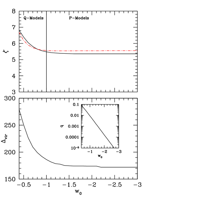
In this case the equation of state is constant (see for a review, Peebles & Ratra 2003; Caldwell 2002; Corasaniti et al. 2004). If $-1\leq w_{0}<-1/3$ we have the so called Quintessence models while for $w_{0}<-1$ we get the so called Phantom cosmologies (hereafter QP-models). Despite the fact that for these models the cluster virialization has been investigated thoroughly in several papers we have decided to re-estimate it in order to understand the variants from the $w=w(t)$ case. In particular, for $w(\alpha)=w_{0}$ we get $f(\alpha)=\alpha^{-3(1+w_{0})}$ and the overall problem (eq. 29) reduces to the integral equation found by Zeng & Gao (2005). In particular, the basic factors become

$$P(y)=\zeta^{1+w_{0}}y^{-3w_{0}-1}$$ (30)

and

$$\Omega_{\rm m}(x)=\frac{1}{1+\nu x^{-3w_{0}}}\;\;.$$ (31)

In Figure 1 we present for the clustered (solid line) and homogeneous dark energy respectively (dashed line) the $\zeta$ solution (top panel), as a function of the equation of state parameter and it is obvious that the two models give almost the same results. Also Figure 1 (bottom panel) shows the dependence of the density contrast at virialization on $w$.

$$\Delta_{\rm vir}=\frac{\rho_{\rm mc,f}}{\rho_{\rm m,f}}=\frac{\zeta}{\lambda^{3}}\left(\frac{\alpha_{\rm f}}{\alpha_{\rm t}}\right)^{3}$$ (32)

where $\rho_{\rm mc,f}$ is the matter density in the virialized structure while $\rho_{\rm m,f}$ is the background matter density at the same epoch. The factor $\Delta_{\rm vir}$ is a key parameter in this kind of studies because we can compare the predictions provided by the spherical collapse model with observations. In this framework, it is also interesting to note that the collapse factor is in between $0.48\leq\lambda\leq 0.50$ while for the homogeneous dark energy we get $0.47\leq\lambda\leq 0.50$. Both cases tend to the standard value $0.5$ in an Einstein de Sitter universe in agreement with previous studies (Maor & Lahav 2005; Wang 2006). This is to be expected simply because at large redshifts matter dominates over the dark energy in the universe which means that the parameter $q$ has small values (see the insert plot of Fig. 1). Note that $\Lambda$-models can be described by quintessence models with $w_{0}$ strictly equal to -1 and thus, eq.(29) is written:

$$\int_{0}^{1}\left[\frac{y}{\zeta+\nu y^{3}-(\zeta+\nu)y}\right]^{1/2}{\rm d}y=\frac{{\rm ln}(\sqrt{1+\nu}+\sqrt{\nu})^{2/3}}{\sqrt{\nu}}\;\;.$$ (33)

Figure 2: The non linear infall velocity in the virialized regime as a function of the equation of state parameter.

In order to explore further the virialized structures we investigate the connection between the infall velocity at the virialized epoch and the equation of state. It is well known from the literature that the non linear infall velocity field is described by the following expression (see Lilje & Efstathiou 1989; Croft, Dalton & Efstathiou 1999):

$$V^{\rm inf}(r)=-\frac{1}{3}H(\alpha)\Omega_{\rm m}^{\beta}(\alpha)r\frac{\delta(r)}{[1+\delta(r)]^{0.25}}\;\;,$$ (34)

where $\delta(r)$ is the fluctuation field. It should be noted that in this work we have used the generic expression for the growth index ($\simeq\Omega_{\rm m}^{\beta}$) defined by Wang & Steinhardt (1998) with

$${\beta}\simeq\frac{3}{5-w_{0}/(1-w_{0})}+\frac{3(1-w_{0})(1-3w_{0}/2)}{125(1-6w_{0}/5)^{3}}(1-\Omega_{\rm m})\;.$$ (35)

Due to interplay between the infall velocity and the virial radius, in Figure 2 we present the corresponding ratio between them at the virialized epoch, [$r=R_{\rm f}$, $\alpha=\alpha_{\rm f}$ and $\delta(R_{\rm f})\simeq\Delta_{\rm vir}$], as a function of the equation of state parameter. Therefore, it becomes evident that for models with $w_{0}<-1$, the so called Phantom models (see Caldwell 2002), the infall velocity is unaffected really by the equation of state. When we use models with $w>-1$ the infall velocity is a decreasing function of $w$ (the difference is $\sim 37\%$). The latter is to be expected because of the $\Delta_{\rm vir}$ behavior (see Figure 1).

4.2 Models with time variation $w$

The last few years there have been many theoretical speculations regarding the nature of the exotic “dark energy”. Various candidates have been proposed in the literature, among which a dynamical scalar field acting as vacuum energy (Ozer & Taha 1987). Under this framework, high energy field theories generically show that the equation of state of such a dark energy is a function of the cosmic time. If this is the case then the basic equations regarding the cluster virilization in models with a time varying equation of state become more complicated than in models with constant $w$. Note that in the literature due to the absence of a physically well-motivated fundamental theory, there is plenty of dark energy models that can fit current observational data (for a review see Liberato & Rosenfeld 2006). In this work as an example, we use several parameterizations regarding the dark energy component in order to evaluate the integrals of eq.(3) and eq. (29). In particular, we consider a simple expression for the equation of state:

$$w(\alpha)=w_{0}+w_{1}X(\alpha)$$

which is available in the literature (see for example Goliath et al. 2001; Linder 2003; Cepa 2004; Liberato & Rosenfeld 2006 and references therein). The function $X(\alpha)$ satisfies the following constrain at the present epoch: $X(1)=0$ and thus, $w_{0}<-1/3$. Here we sample the parameters as follows: $w_{0}\in[-1.05,-0.35]$ and $w_{1}\in[0.1,1.5]$ in steps of 0.1. To this end, we need to emphasize that our approach is powerful in a sense that for different parametric forms of $w(\alpha)$ the system of eq. (19) and eq. (20) can be solved analytically in the framework of a clustered dark energy. Finally, in this work we assume that the parameters $(w_{0},w_{1})$ and the functional form of the equation of state parameter remain the same either for the entire universe or for the spherical perturbations.

4.2.1 The $w(\alpha)=w_{0}+w_{1}(1-\alpha)$ model

In this case, (see Linder 2003; Cepa 2004) where $w_{0}$ and $w_{1}$ are constants, using eq.(3), eq.(24) and eq.(28) we derive the following basic functions of the differential equation eq.(29):

$$f(\alpha)=\alpha^{-3(1+w_{0}+w_{1})}e^{3w_{1}(\alpha-1)}$$ (36)

$$\Omega_{\rm m}(x)=\frac{1}{1+\nu x^{-3(w_{0}+w_{1})}e^{3w_{1}(x-1)}}$$ (37)

and

$$P(y)=\frac{\zeta^{1+w_{0}+w_{1}}e^{3w_{1}\alpha_{\rm t}(\zeta^{-1/3}y-1)}}{y^{3(w_{0}+w_{1})+1}}\;\;.$$ (38)

Figure 3: Possible pairs $(w_{0},w_{1}$) defining the collapse factor $\lambda$ for the clustered case, based on $w(\alpha)=w_{0}+w_{1}(1-\alpha)$ [see section 4.2.1]. The lines correspond to $w_{0}=-0.35$ (solid), $w_{0}=-0.45$ (short dashed), $w_{0}=-0.55$ (dashed) and $w_{0}=-0.65$ (dot dashed).

For the homogeneous dark energy scenario we find that the collapse factor lies in the range $0.47\leq\lambda\leq 0.50$ while for the clustered case we get $0.30\leq\lambda\leq 0.50$. In particular, Fig.3 shows the behavior of the collapse factor for possible pairs of $(w_{0},w_{1}$) starting from $w_{0}=-0.35$ (solid line), $w_{0}=-0.45$ (short dashed line), $w_{0}=-0.55$ (dashed line) and $w_{0}=-0.65$ (dot dashed line). From the figure, it becomes evident that for large values of $w_{1}$ the collapse factor is significant less than 0.5 which means that under the framework of the present equation of state, a candidate structure (large scale overdensity) is located in a large density regime ($\Delta_{\rm vir}>400$) and at the end the tendency is to collapse in a more bound system, with respect to the QP-models ($w=const$). Additionally, it is interesting to mention that for small values of $w_{1}<0.55$ the structures reveal a similar dynamical behavior, $0.48\leq\lambda\leq 0.50$, as described in section 4.1.

4.2.2 The $w(\alpha)=w_{0}+w_{1}(\alpha^{-1}-1)$ model

Using now the equation of state derived by Goliath et al. (2001) then the formulas described before become:

$$f(\alpha)=\alpha^{-3(1+w_{0}-w_{1})}e^{3w_{1}(\alpha^{-1}-1)}$$ (39)

$$\Omega_{\rm m}(x)=\frac{1}{1+\nu x^{-3(w_{0}-w_{1})}e^{3w_{1}(x^{-1}-1)}}$$ (40)

and

$$P(y)=\frac{\zeta^{1+w_{0}-w_{1}}e^{3w_{1}\alpha^{-1}_{\rm t}(\zeta^{1/3}y^{-1}-1)}}{y^{3(w_{0}-w_{1})+1}}\;\;.$$ (41)

Following the same paradigm as in the previous case in Fig.4 we present for the clustered case the distribution of $\lambda$. It is obvious that also this equation of state affects the virialization of the large scale structures in the same way as before (see section 4.2.1), but the corresponding $w_{1}$ parameter takes much lower values. For $w_{1}<0.15$ the collapse factor tends to 0.5. Note, that for the homogeneous dark energy the collapse factor is in the range $0.45\leq\lambda\leq 0.49$.

Figure 4: The collapse factor $\lambda$, based on $w(\alpha)=w_{0}+w_{1}(\alpha^{-1}-1)$ [see section 4.2.2]. The lines correspond to the same values of $w_{0}$ as in figure 3.

4.2.3 The $w(\alpha)=w_{0}+w_{1}(1-\alpha)\alpha$ model

In this case, (see Liberato & Rosenfeld 2006) we get:

$$f(\alpha)=\alpha^{-3(1+w_{0})}e^{\frac{3w_{1}}{2}(\alpha-1)^{2}}$$ (42)

$$\Omega_{\rm m}(x)=\frac{1}{1+\nu x^{-3w_{0}}e^{\frac{3w_{1}}{2}(x-1)^{2}}}$$ (43)

and

$$P(y)=\frac{\zeta^{1+w_{0}}e^{\frac{3w_{1}}{2}\alpha_{\rm t}(\alpha_{\rm t}\zeta^{-2/3}y^{2}-\alpha_{\rm t}-2\zeta^{-1/3}y+2)}}{y^{3w_{0}+1}}\;\;.$$ (44)

Performing once again the same constrains as before the virialization radius to the turn around radius lies in the range $0.46\leq\lambda\leq 0.50$. This result is in agreement with those derived in the QP-models, despite the fact that the two dark energy models have completely different equations of state. Finally, considering now the homogeneous dark energy scenario the collapse factor is almost in the same interval i.e, $0.45\leq\lambda\leq 0.48$.

5 Conclusions

The launch of the recent observational data has brought great progress in understanding the physics of gravitational collapse as well as the mechanisms that have given rise to the observed large-scale structure of the universe. In this work assuming that the dark energy moves synchronously with ordinary matter on both the Hubble scale and the galaxy cluster scale (clustered dark energy), we have treated analytically the nonlinear spherical collapse scenario considering different models with negative pressure which contains also a time varying equation of state. We verify that having an overdense region of matter, which will create a cluster of galaxies prior to the epoch of $z_{\rm f}\simeq 1.4$, dark energy affects the virialization of the large scale structures in the following manner: flat cosmological models that contain either (i) a constant equation state or (ii) an equation of state with $w=w_{0}+w_{1}(1-\alpha)\alpha$ the virialization radius divided by the turn around radius is in between $0.47\leq R_{\rm f}/R_{\rm t}\leq 0.50$ and the density contrast at virialization lies in the interval $171\leq\Delta_{\rm vir}\leq 240$. It is interesting to mention that the same behavior is also found for the homogeneous dark energy. Finally, we find that the following equations of state: $w=w_{0}+w_{1}(1-\alpha)$ and $w=w_{0}+w_{1}(\alpha^{-1}-1)$ correspond to relative larger $\Delta_{\rm vir}$’s and thus, produce more bound systems ($0.30\leq R_{\rm f}/R_{\rm t}\leq 0.50$) with respect to the other two equations of state mentioned before. While for the homogeneous dark energy we found structures where the collapse factor is in between $0.45\leq R_{\rm f}/R_{\rm t}\leq 0.49$.

Appendix A

Without wanting to appear too pedagogical, we remind the reader of some basic elements of Algebra. Given a cubic equation: $\lambda^{3}+a_{1}\lambda^{2}+a_{2}\lambda+a_{3}=0$, let ${\cal}D$ be the discriminant:

$${\cal D}=a_{1}^{2}a_{2}^{2}-4a_{2}^{3}-4a_{1}^{3}a_{3}-27a_{3}^{2}+18a_{1}a_{2}a_{3}$$ (45)

and

$$x_{1}=-a_{1}^{3}+\frac{9}{2}a_{1}a_{2}-\frac{27}{2}a_{3}\;,\;\;\;\;\;\;x_{2}=-\frac{3\sqrt{3\cal{D}}}{2}\;\;.$$

If ${\cal D}>0$, all roots are real (irreducible case). In that case $\lambda_{1}$, $\lambda_{2}$ and $\lambda_{3}$ can be written:

$$\lambda_{\mu}=-\frac{a_{1}}{3}-\frac{2r^{1/3}}{3}{\rm cos}\left[\frac{\theta-(\mu-1)\pi}{3}\right]\;\;\;\;\;\;\mu=1,2,3$$ (46)

where $r=\sqrt{x_{1}^{2}+x_{2}^{2}}$ and $\theta={\rm cos^{-1}}(x_{1}/r)$.

In this study, we derive analytically the exact solution of the basic cubic equation (eq.15), having polynomial parameters: $a_{1}=0$, $a_{2}=-(1+q)/2q$ and $a_{3}=1/4q$. Then the discriminant of eq.(15) is:

$${\cal D}(q)=\frac{8(1+q)^{3}-27q^{2}}{16q^{3}}\;\;.$$

Of course, in order to obtain physically acceptance results we need to take $q>0$ which gives ${\cal D}(q)>0$. Therefore, all roots of the cubic equation are real (irreducible case) but one of them $\lambda_{3}$ corresponds to expanding shells. It is obvious that for $q\longrightarrow 0$ the above solution tends to the Einstein-de Sitter case ($\lambda_{3}\longrightarrow 0.50$), as it should.

Appendix B

We present here some more details regarding the integration of eq. (26). Considering a spherical overdensity with radius $R$ the functional form of eq.(3) becomes:

$$f(R)={\rm exp}\left[3\int_{R}^{1}\left(\frac{1+w(u)}{u}\right){\rm d}u\right]\;\;.$$ (47)

Taking now into account that $R(y)=R_{\rm t}y=\zeta^{-1/3}\alpha_{\rm t}y$, (described well in section 3.1) and differentiating the above integral we have the following useful formula:

$$\frac{{\rm d}f(R(y))}{{\rm d}y}=\frac{{\rm d}f}{{\rm d}R}\frac{{\rm d}R}{{\rm d}y}=-3y^{-1}[1+w(R(y))]f(R(y))\;.$$ (48)

Using now the integral of eq. (26)

$$\begin{array}[]{rcl}\int y[1+3w(R(y))]f(R(y)){\rm d}y=-2\int yf(R(y)){\rm d}y\\ +3\int[1+w(R(y))]yf(R(y)){\rm d}y\end{array}$$ (49)

and taking into account eq. (48) we can easily solve the integral

$$\begin{array}[]{rcl}\int y[1+3w(R(y))]f(R(y)){\rm d}y=-2\int yf(R(y)){\rm d}y\\ -\int y^{2}\frac{{\rm d}f(R(y))}{{\rm d}y}{\rm d}y=-y^{2}f(R(y))\end{array}$$ (50)

References

- [] Bartelmann M., Doran M., &, Wetterich, C., 2006, A&A, 454, 27
- [] Basilakos S., 2003, ApJ, 590, 636
- [] Basilakos S., &, M. Plionis M., MNRAS, 2005 360, L35
- [] Battye R. A., &, Weller J., Phys. Rev. D, 2003, 68, 3506
- [] Caldwell R. R., Dave R., Steinhardt P. J., Phys. Rev. Lett., 1998, 80, 1582
- [] Caldwell, R. R., Phys. Let. B, 2002, 545, 23
- [] Cepa J., A&A, 2004, 422, 831
- [] Corasaniti, P. S., Kunz, M., Parkinson, D., Copeland. E. J., &, Bassett, B. A., Phys. Rev. D, 2004, 70, 3006
- [] Croft, R. A. C., Dalton, G. B., &, Efstathiou, G., MNRAS, 1999, 305, 547
- [] Freedman W. L., et al., ApJ, 2001, 553, 47
- [] Gunn J. E., &, Gott J. R., ApJ, 1972 176, 1
- [] Goliath A., Amanulah R., Astier P., Goobar A, &, Pain R., A&A, 2001, 380, 6
- [] Horellou C., &, Berge J., 2005, MNRAS, 360, 1393
- [] Iliev I. T., &, Shapiro P. R., 2001, MNRAS, 325, 468
- [] Lahav O., Lilje P. B., Primack J. R., &, Rees M. J., MNRAS, 1991, 251, 128
- [] Liberato, L., &, Rosenfeld, R., 2006, JCAP, 7, 9
- [] Lilje P. B., &, Efstathiou, G., MNRAS, 1989, 236, 851
- [] Linder E. V., Phys. Rev. Lett., 2003, 90, 1301
- [] Lokas E. L., Acta Physica Polonica B, 2001, 32, 3643
- [] Mainini, R., Maccio, A. V., Bonometto, S. A., &, Klypin, A., ApJ, 2003, 599, 24,
- [] Maor I., &, Lahav O., Journal of Cosmology and Astroparticle Physics, 2005, 7, 3
- [] Mota D. F., &, van de Bruck C., A&A, 2004, 421, 71
- [] Mullis C. R., Rosati P., Lamer G., Behringer H., Schuecker P., &, Fassbender R., MNRAS, 2005, 623, L85
- [] Nunes N. J., &, Mota D. F., MNRAS, 2006, 368, 751
- [] Ozer, M., &, Taha, O., Nucl. Phys. B, 1987, 287, 776
- [] Peebles P. J. E., &, Ratra B., RvMP, 2003, 75, 559
- [] Percival W. J., A&A, 2005, 443, 819
- [] Ratra B., &, Peebles P. J. E., Phys. Rev. D, 1988, 37, 3406
- [] Spergel D. N., et al., ApJS, 2003, 148, 175
- [] Spergel D. N., et al., ApJ, 2006, submitted, (astro-ph/0603449)
- [] Stanford, S. A., et al., ApJ, 2006, 646, L13
- [] Tegmark M., et al. , Phys. Rev. D, 2004, 69, 3501
- [] Wang L., &, Steinhardt P. J., ApJ, 1998, 508, 483
- [] Wang P., ApJ, 2006, 640, 18
- [] Weinberg N. N., &, Kamionkowski M., ApJ, 2003, 341, 251
- [] Zeng, Ding-fang, &, Gao, Yi-hong., 2005, (astro-ph/0505164)