Observations of High-Redshift X-Ray Selected Clusters with the Sunyaev-Zel’dovich Array

Abstract

We report measurements of the Sunyaev-Zel’dovich (SZ) effect in three high-redshift ($0.89\leq z\leq 1.03$), X-ray selected galaxy clusters. The observations were obtained at 30 GHz during the commissioning period of a new, eight-element interferometer – the Sunyaev-Zel’dovich Array (SZA) – built for dedicated SZ effect observations. The SZA observations are sensitive to angular scales larger than those subtended by the virial radii of the clusters. Assuming isothermality and hydrostatic equilibrium for the intracluster medium, and gas-mass fractions consistent with those for clusters at moderate redshift, we calculate electron temperatures, gas masses, and total cluster masses from the SZ data. The SZ-derived masses, integrated approximately to the virial radii, are $1.9^{+0.5}_{-0.4}\times 10^{14}M_{\odot}$ for Cl J1415.1+3612, $3.4^{+0.6}_{-0.5}\times 10^{14}M_{\odot}$ for Cl J1429.0+4241 and $7.2^{+1.3}_{-0.9}\times 10^{14}M_{\odot}$ for Cl J1226.9+3332. The SZ-derived quantities are in good agreement with the cluster properties derived from X-ray measurements.

1 Introduction

Galaxy clusters are the most massive, gravitationally-bound structures in the Universe. Over a Hubble time, they form from the rare, high-density peaks in the primordial density field on scales of $\sim 10~{}{\rm Mpc}$. As their abundance and evolution are critically dependent on cosmology, there is considerable interest in finding clusters at high redshift ($z\geq 1$). To date, only a few massive clusters at $z>1$ have been identified and confirmed, primarily through the detection of extended X-ray emission from the hot intracluster medium (ICM) (e.g., Mullis et al. 2005; Bremer et al. 2006; Maughan et al. 2006; Stanford et al. 2006). In addition to X-ray observations, optical and infrared observations of the cluster member galaxies, and weak lensing of background galaxies by the deep cluster potential, are complementary probes of high-redshift clusters (e.g., Refregier 2003; Gladders et al. 2006; Stanford et al. 2005; Clowe et al. 2006; Wittman et al. 2006).

Recently, Sunyaev-Zel’dovich effect measurements of galaxy clusters have emerged as a powerful probe of cluster physics and cosmology (for a review, see Carlstrom et al. 2002). Measurements of the SZ effect have been used to determine cluster properties such as the gas and total masses, electron temperatures and scaling relations, as well as to constrain $H_{0}$ and the cosmological distance scale (e.g., Hughes & Birkinshaw 1998; Mason et al. 2001; Grego et al. 2001; Reese et al. 2002; McCarthy et al. 2003; Benson et al. 2004; Jones et al. 2005; Afshordi et al. 2005; LaRoque et al. 2006; Bonamente et al. 2006). Several telescopes specifically designed for observations of the SZ effect in high-redshift clusters are currently operating or under development, including the Sunyaev-Zel’dovich Array, the Arcminute Microkelvin Imager (Kaneko 2006), the Atacama Cosmology Telescope (Fowler 2004) and the South Pole Telescope (Ruhl et al. 2004).

The SZ effect is a spectral distortion of the cosmic microwave background (CMB) radiation caused by inverse Compton scattering of the CMB photons by electrons in the hot ICM (Sunyaev & Zel’dovich 1970, 1972, see also Birkinshaw 1999). The magnitude of the effect is proportional to the integrated pressure of the ICM, i.e., the density of electrons along the line of sight, weighted by the electron temperature. The SZ flux of a cluster is therefore a measure of its total thermal energy.

The change in the observed brightness of the CMB caused by the SZ effect is given by

$$\frac{\Delta T_{\rm CMB}}{T_{\rm CMB}}=f(x)\int\sigma_{\rm T}n_{e}\frac{k_{B}T_{e}}{m_{e}c^{2}}dl\equiv f(x)y$$ (1)

where $T_{\rm CMB}$ is the cosmic microwave background temperature (2.73 K), $\sigma_{\rm T}$ is the Thomson scattering cross section, $k_{B}$ is Boltzmann’s constant, $c$ is the speed of light, and $m_{e}$, $n_{e}$, and $T_{e}$ are the electron mass, number density and temperature. Equation (1) defines the Compton $y$-parameter. The frequency dependence of the SZ effect is contained in the term

$$f(x)=\left(x\frac{e^{x}+1}{e^{x}-1}-4\right)\left(1+\delta_{\rm SZ}(x,T_{e})\right),$$ (2)

where $x\equiv h\nu/{k_{B}T_{\rm CMB}}$, $h$ is Planck’s constant, and $\delta_{\rm SZ}$ is a relativistic correction, for which we adopt the Itoh et al. (1998) calculation, valid to fifth order in $k_{B}T_{e}/m_{e}c^{2}$. The SZ effect appears as a temperature decrement at frequencies below $\approx 218~{}{\rm GHz}$, and an increment at higher frequencies.

The redshift independence of the SZ effect in both brightness and frequency (the ratio $\Delta T/T$ in equation (1) is independent of the distance to the cluster) offers enormous potential for finding high-redshift clusters. A cluster catalog resulting from an SZ survey of uniform sensitivity will be limited by a cluster mass threshold that is only weakly dependent on redshift for $z\gtrsim 0.5$ (via the angular diameter distance). To realize the full potential of SZ surveys for cosmology will require a thorough understanding of the relationship between SZ observables and cluster mass, achievable through detailed cluster observations.

The SZA is a new, eight-element array of 3.5-meter precision telescopes designed to conduct SZ surveys at 30 GHz and detailed cluster observations at 30 GHz and 90 GHz. We present observations obtained during the commissioning of the SZA, of three high-redshift, X-ray selected clusters: ClJ1226.9+3332 at $z=0.89$, ClJ1429.0+4241 at $z=0.92$ and ClJ1415.1+3612 at $z=1.03$. We describe the analysis of the SZ data and compare the derived cluster properties with those determined from X-ray observations. We also compare the SZA observations of ClJ1226.9+3332 with previous BIMA observations of the SZ effect (Joy et al. 2001) in the same cluster. No previous SZ measurements of the other two clusters have been reported.

The paper is organized as follows: In §2 we describe the Sunyaev-Zel’dovich Array, followed by a description of the data acquisition, reduction and calibration. The data analysis is presented in §3. In §4 we present the results of the analysis and compare with previous SZ and X-ray results. Conclusions are given in §5.

2 Observations and Data Reduction

2.1 The Sunyaev-Zel’dovich Array

The Sunyaev-Zel’dovich Array (SZA) is a new interferometer equipped with sensitive centimeter (26–36 GHz) and millimeter-wavelength (80–115 GHz) receivers, designed specifically for detecting and imaging the SZ effect in galaxy clusters. In this paper, we report results only from the centimeter-wavelength (hereafter 30 GHz) SZA observations.

An interferometer has sensitivity to angular scales up to the resolution of its shortest baseline. To provide a good match to galaxy clusters, which at $z\gtrsim 0.1$ subtend several arcminutes on the sky, the SZA was designed with small (3.5 meter) antennas, allowing close-packed configurations with sensitivity to scales as large as $5\arcmin$ at 30 GHz. The specific choice of diameter provides optimum brightness sensitivity to the SZ effect from distant clusters, while filtering out the contamination by the intrinsic anisotropy of the CMB at larger angular scales. The instantaneous field of view of the SZA is given by the primary beam of the 3.5-meter antennas, approximately $12\arcmin$ (FWHM) at 30 GHz.

Six of the SZA antennas are arranged in a close-packed configuration with separations (baselines) ranging from $4.5-11.5~{}{\rm m}$ ($0.3-1.3~{}{\rm k\lambda}$ at 30 GHz), yielding high brightness sensitivity, and a resolution of $\sim 2\arcmin$, for the detection of the SZ effect in clusters (see Fig. 1). Two outer telescopes, one to the north and one to the northeast of the central array, yield baselines of up to $65~{}{\rm m}$ ($7.7~{}{\rm k\lambda}$ at 30 GHz) to facilitate simultaneous to optimize the surveying speed detection of contaminating compact sources at a resolution of $\sim 0.3\arcmin$. This hybrid configuration was chosen to optimize the surveying speed of the SZA in an untargeted search. Detailed imaging of the SZ effect can be achieved with alternate telescope configurations and with SZA observations at 90 GHz.

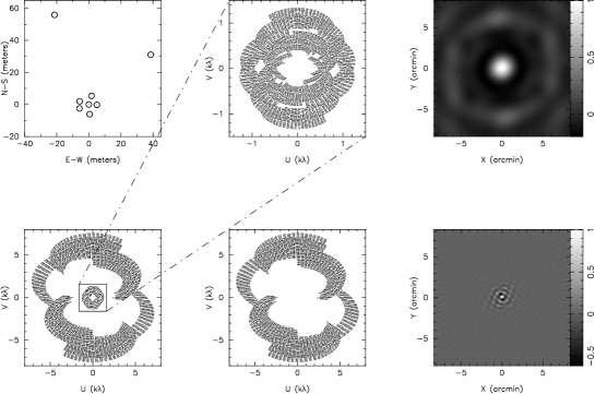
Figure 1: Top left: SZA telescope locations. Bottom left: Resulting Fourier-space ($u$-$v$) coverage for a single track (all baselines). Top middle: $u$-$v$ coverage for the short-baselines only ($0-2~{}{\rm k\lambda}$). Bottom middle: $u$-$v$ coverage for the long baselines only ($2-8~{}{\rm k\lambda}$). Top right: resulting point spread function (synthesized beam), short-baselines. Bottom right: synthesized beam, long baselines.

The SZA centimeter-wave receivers use cryogenic $26-36~{}{\rm GHz}$ high electron mobility transistor (HEMT) amplifiers (Pospieszalski et al. 1995), with characteristic receiver temperatures $T_{rx}\sim 11-20~{}{\rm K}$. Typical system temperatures, including atmospheric contributions, range from $\sim 30-60~{}{\rm K}$ in the 8-GHz band from $27$ to $35~{}{\rm GHz}$, used for these observations. Optical fibers transport the signal (mixed down to intermediate frequencies of $1-9~{}{\rm GHz}$) to a wideband hybrid correlator. Sixteen 500 MHz-wide analog bands are further divided into seventeen $31.25~{}{\rm MHz}$ channels by 2-bit digital lag correlators, providing spectral discrimination as well as high-sensitivity broadband measurements. Additionally, the wide fractional bandwidth broadens the Fourier-space ($u$-$v$) coverage appreciably, as is evident in Fig. 1.

2.2 Observations

Clusters were typically observed for 10 hours about transit, which we refer to as a track. Observations of the clusters were interleaved with observations of a strong unresolved source every 15 minutes, to monitor variations in the instrumental gain. Cl J1415.1+3612 was observed for a total of 15 tracks from August 23 to October 8, 2005, using J1331+305 as its calibrator. Cl J1429.0+4241 was observed for a total of 15 tracks between September 30 and October 28, 2005, also using J1331+305 as its calibrator. Cl J1226.9+3332 was observed for 3 tracks between August 30 and September 4, 2005, using J1310+323 as its calibrator.

Data were calibrated and excised (flagged) in a data reduction package specific to the SZA (see Section 2.3). Data in this paper were taken during the commissioning period of the array, during which $\sim 44\%$ of the data were flagged. Causes of flagging were: an offline antenna ($17\%$); shadowing of one antenna by another ($15\%$); corruption of one 500-MHz band ($6\%$); lack of bracketing calibrator observations ($\sim 5\%$), and rare, spurious correlations ($<1\%$). Subsequent improvements to the instrument and observing strategy have reduced flagged data to $<5\%$ in good weather conditions.

In Table 1, we give the pointing center and cluster redshift for each observation (taken from Maughan et al. (2006)), along with details of the observations, including the synthesized beam sizes (see §3) for both the short and long baselines. We also present the achieved rms flux sensitivities for maps made with short and long-baseline data, and the corresponding brightness temperature sensitivities for the short-baseline maps. The rms in the short-baseline maps is expected to be marginally lower than those of the long baselines (since there are 15 short baselines and 13 long baselines). For some of the observations of Cl J1415.1+3612 and Cl J1429.0+4241, however, one of the inner telescopes was offline, resulting in a larger number of long baselines than of short baselines.

Table 1: Cluster Observations

Cluster Name	$z$	Pointing Center (J2000)		$\rm{t_{int}}$	$\rm{T_{sys}}$	Short Baselines (0-1.5k$\lambda$)			Long Baselines (2-8k$\lambda$)
		$\alpha$	$\delta$	(hrs)	(K)	beam($\arcsec\times\arcsec\angle$)	$\sigma$(mJy)	B($\mu$K)	beam($\arcsec\times\arcsec\angle$)	$\sigma$(mJy)
Cl J1415.1+3612	1.03	14h15m11s.2	36∘12′04′′	34.1	41.9	115.4$\times$131.2 -61.1	0.16	13.5	15.7$\times$21.4 87.2	0.16
Cl J1429.0+4241	0.92	14h29m06s.4	42∘41′10′′	32.1	41.7	109.9$\times$136.9 -60.9	0.17	13.6	15.6$\times$21.3 83.1	0.16
Cl J1226.9+3332	0.89	12h26m58s.0	33∘32′45′′	7.6	42.9	117.4$\times$125.4 -64.8	0.38	32.9	16.0$\times$21.2 79.2	0.37

2.3 Data Reduction and Calibration

The SZA data reduction package consists of a suite of MATLAB routines, which constitute a complete pipeline for flagging, calibrating, and reducing visibility data (see §3) before input to higher-level analysis software. In the pipeline, data are converted to physical units and corrected for instrumental phase and amplitude variations. Calibration is performed using antenna-based gain solutions; data are flagged if they do not meet designated criteria at each reduction step. The pipeline outputs the calibrated, unflagged cluster visibility data.

The output of the correlator is a complex, dimensionless correlation coefficient — the ratio of correlated power to total power for each baseline. To convert these values to physical units (K), we first calculate the system temperature of the antennas by comparison with two loads of known temperature (a blackbody calibrator load on the telescope, and the CMB). System temperature measurements are made at the beginning and end of every scan, where scans are defined as the short (typically 5 to 15 minute) observations of either the cluster or the calibrator within a track. Data for a scan are written to disk in consecutive $20$-second integrations, which is the native timescale on which calibration, flagging and Fourier-space calculations are performed. Data with high system temperatures (an indication of poor weather), or spurious calibration values (due to readout error of the power sensors) are flagged at this stage of the data reduction.

Absolute calibration is derived from observations of Mars, using fluxes predicted by the Rudy model (Rudy 1987). Since Mars is partially resolved on the longest baselines, a strong, unresolved source is used to transfer the calibration from the short baselines. This absolute flux calibration is performed bimonthly. Measured antenna efficiencies (which include aperture efficiencies, atmospheric and system phase noise, correlator efficiencies, and other factors) have fluctuated by less than 5% in the period for which the data in this paper were taken. The absolute calibration was cross-checked by comparing SZA observations of Jupiter to those of WMAP and CBI (Page et al. 2003; Readhead et al. 2004). Based on these measurements, we estimate the absolute flux calibration to be better than 10% during these observations.

Bandpasses are measured at the beginning of every track using a flat-spectrum, unresolved radio source with high signal-to-noise in each 31.25-MHz channel. The first and last 31.25-MHz channel of each 500-MHz band are flagged, as they are corrupted by aliasing in the lag correlator. The bandpasses are corrected to remove differential gain (amplitude and phase) across the channels within each 500-MHz band, and the absolute flux calibration on Mars removes differential gain amplitude across the sixteen 500-MHz bands. This leads to a uniform gain calibration across the entire $8~{}{\rm GHz}$ bandwidth.

The phase from the changing geometric delay as a source is tracked across the sky is removed in hardware by inducing a phase shift in the local oscillator signal at each antenna, and digitally, in the lag correlator, to account for the bandwidth. Accurate removal of the geometric delay, which impacts the dynamic range of the instrument as well as the accuracy to which source positions can be measured, requires precise knowledge of each telescope location, as well as a measurement of the displacement of the azimuth and elevation axes of the telescopes. These locations have been determined to $<0.1~{}\rm{mm}$ by direct measurements and by observations of a set of strong radio sources across the sky.

To remove residual instrumental phases, a strong unresolved source is observed every 15 minutes (over which time the instrumental phase variations are typically much less than $35^{\circ}$). The interpolated calibrator phase is removed on a per-antenna basis; data are flagged if it is not possible to interpolate the phase, either because a calibrator observation is bad or because bracketing observations are missing. Data are also flagged if a phase jump of more than $35^{\circ}$ is observed between calibrator pointings. Observations of the phase calibrator are reused to perform a relative amplitude calibration across a given track, to check for any time-varying antenna gain. We have seen no indication that the gain on an individual antenna changes significantly on timescales less than 12 hours. The gain amplitudes are scaled so that the time-average of the gain over a track is the same for all antennas.

3 Data Analysis

In the limit where sky curvature is negligible over the instrument’s field of view, the response of an interferometer on a single baseline, known as a visibility, can be approximated by:

$$V(u,v)=\int_{-\infty}^{+\infty}\int_{-\infty}^{+\infty}A_{N}(l,m)I(l,m)\times\exp\{-2\pi j[ul+vm]\}{dl\,dm},$$ (3)

where $u$ and $v$ are the baseline lengths projected onto the sky, $l$ and $m$ are direction cosines measured with respect to the $(u,v)$ axes, $A_{N}(l,m)$ is the normalized antenna beam pattern, and $I(l,m)$ is the sky intensity distribution.

As implied by equation (3), an image of the source intensity multiplied by the antenna beam pattern, also known as a dirty map, can be recovered by Fourier transform of the visibility data. Note that in addition to modulation by the primary beam, structure in the dirty map is convolved with a function that reflects the incomplete Fourier-space sampling of a given observation. This filter function is the synthesized beam (see Figure 1), equivalent to the point-spread function for the interferometer. The unprocessed maps shown in the first four columns of Fig. 2 are examples of dirty maps. A $clean$ map, such as the ones in the last column of Fig. 2, is an image from which the full synthesized beam pattern has been deconvolved, and the source model reconvolved with a Gaussian fit to the central lobe of the synthesized beam. Where a resolution is quoted in this paper, it is this fitted Gaussian that is indicated.

All quantitative analyses described in this paper are the result of simultaneously fitting models of the SZ cluster decrement and sources of contaminating emission — both point-like and extended — as detailed below. In all cases, the model is constructed in the sky-plane and then multiplied by the primary beam across the field of view. After performing a Fourier transform (as given by equation (3)), the resulting model visibilities are compared directly to the SZA data. In this way all fitting is done in the Fourier-plane, where the noise characteristics and the spatial filtering of the interferometer are well understood; maps are used only for examination of the data and to identify cases where contaminating sources are present. The two distinct ranges in Fourier-space coverage demonstrated in Figs. 1 and 2 facilitate removal of sources unresolved by the long-baseline synthesized beam (point sources from the perspective of our instrument). Constraints on the point-source flux come primarily from baselines including one or both of the outer telescopes, which probe small scales where the cluster signal is exponentially damped, while the compact inner array provides sensitivity to extended emission.

The frequency-dependent shape of the primary beam used in the analysis is calculated from the Fourier transform of the aperture illumination of each Cassegrain telescope. The illumination is modeled as a Gaussian taper, with a central obscuration corresponding to the secondary mirror; the validity of this model has been confirmed by holographic measurements of the primary mirrors.

Table 2: Unresolved Radio Sources

Cluster Field	$\#$	$RA$	$\sigma_{\rm RA}$	$DEC$	$\sigma_{\rm DEC}$	d	31 GHz Flux	$\alpha$	1.4 GHz flux	$\alpha$
		(J2000)	(s)	(J2000)	(″)	(′)	(mJy)		(mJy)	(1.4/31 GHz)
Cl J1415.1+3612	1	$14^{h}15^{m}11^{s}.28$	0.12	$+36^{\circ}12^{\prime}05^{\prime\prime}.1$	1.2	0.02	$0.91\pm 0.15$		$3.15\pm 0.21$	$0.40\pm 0.06$
	2	$14^{h}15^{m}07^{s}.43$	0.13	$+36^{\circ}16^{\prime}17^{\prime\prime}.0$	1.3	4.28	$1.01\pm 0.17$		$1.28\pm 0.16$	$0.08\pm 0.07$
Cl J1429.0+4241	1	$14^{h}28^{m}32^{s}.65$	0.01	$+42^{\circ}40^{\prime}20^{\prime\prime}.8$	0.1	6.26	$26.11\pm 0.32$	$0.42\pm 0.17$	$43.6\pm 2.2$	$0.17\pm 0.02$
	2	$14^{h}28^{m}46^{s}.14$	0.15	$+42^{\circ}38^{\prime}11^{\prime\prime}.4$	1.2	4.77	$1.38\pm 0.21$		$4.04\pm 0.24$	$0.35\pm 0.05$
Cl J1226.9+3332	1	$12^{h}27^{m}18^{s}.63$	0.08	$+33^{\circ}32^{\prime}06^{\prime\prime}.6$	0.7	4.35	$4.56\pm 0.42$	$1.1\pm 1.4$	$23.2\pm 1.2$	$0.53\pm 0.03$

3.1 Point Source Extraction

When fitting an unresolved radio source, hereafter referred to as a point source, we represent it by a delta function, parameterized by the intensity at the band center, $I_{31\,{\rm GHz}}$, and a spectral index $\alpha$ over our sixteen $500~{}\rm{MHz}$-wide correlator bands. The point source intensity at frequency $\nu$ is then:

$$I_{ps}(l,m)=I_{31\,{\rm GHz}}\times\left(\frac{\nu}{{31\,{\rm GHz}}}\right)^{-\alpha}\delta(l-l^{\prime})\,\delta(m-m^{\prime}),$$ (4)

where $l^{\prime}$ and $m^{\prime}$ are the coordinates of the point source on the sky. From equations (3) and (4), it can be seen that the visibility amplitude due to a point source is simply its intensity, weighted by the normalized primary beam response at the source location.

The Cl J1415.1+3612 and Cl J1429.0+4241 cluster fields were each found to contain two point sources, while only one point source was detected in the Cl J1226.9+3332 field (see Table 2 and Fig. 2). All detected point sources have counterparts in the 1.4 GHz FIRST catalog (White et al. 1997). Spectral indices of sources detected with high signal-to-noise can be constrained using SZA data alone (see Table 2, where the limiting signal-to-noise is indicated by the poor constraint on the spectral index of the last source listed). The spectral indices of weaker sources are not well constrained by our data; for these sources the spectral index was fixed to the value determined from the integrated flux at 1.4 GHz and the fitted total flux at 31 GHz. The strong source in the Cl J1429.0+4241 field provides a good test of our ability to extract point sources. Following removal of this source from fits to the long-baseline data alone, we obtain source flux residuals of less than 3% in both the long and short baseline maps.

3.2 Extended Source Extraction

Where an extended source of emission is present in the field, its frequency dependence is modeled as in equation (4), with spatial extent given by an elliptical Gaussian. One such object, identified as the edge-on spiral galaxy NGC 5529, was detected in the Cl J1415.1+3612 field. The fitted source parameters are in good agreement with the NVSS survey (Condon et al. 1998), which detects a source $\sim 2\arcmin$ in extent, at a position angle of $-64^{\circ}$, with an unresolved minor axis. Comparison of the integrated 31 GHz flux for this object ($2.55\pm 0.22$ mJy) with the integrated flux from the NVSS catalog yields a spectral index $\alpha_{\rm 1.4~{}GHz/{31\,{\rm GHz}}}=0.64\pm 0.04$, consistent with synchrotron emission. Fig. 2 shows the effect of removing both point sources and this extended emission from the Cl J1415.1+3612 cluster field.

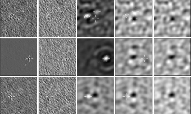
Figure 2: Radio source subtraction in our three cluster observations. The rows, from top to bottom, depict observations of Cl J1415.1+3612, Cl J1429.0+4241, and Cl J1226.9+3332. The first column shows the dirty map of the long-baseline data ($u$-$v$ radii $>2~{}{\rm k\lambda}$). The second column shows the same maps, with fitted point sources removed, as discussed in §3.1, resulting in map residuals consistent with noise. The locations of fitted point sources are indicated with cross-hairs. The third column shows the dirty map made from the short baseline data ($u$-$v$ radii $<2~{}{\rm k\lambda}$). The fourth column shows the same maps, following the removal of all sources of radio emission. In the top panel (Cl J1415.1+3612), we have removed the extended emission from NGC 5529, indicated by an ellipse, resolved out in the long-baseline map. The resulting cluster decrements reflect the shape of the synthesized beam (see §3 and Fig. 1), convolved with the intrinsic cluster profile. The final column shows the clean map of the SZ decrement in each cluster. Images are $\approx 21\arcmin$ on a side, nearly twice the FWHM of the primary beam.

3.3 Cluster Parameter Estimation

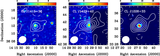
Figure 3: Sunyaev-Zel’dovich Effect measurements (contours) overlaid on X-ray images (halftone) of Cl J1415.1+3612, Cl J1429.0+4241, and Cl J1226.9+3332. The contours are set at brightness levels corresponding to integer multiples of $\pm 20~{}{\rm\mu K}$ for Cl J1415.1+3612, $\pm 20~{}{\rm\mu K}$ for Cl J1429.0+4241 and $\pm 49~{}{\rm\mu K}$ for Cl J1226.9+3332, corresponding to $\pm 1.5$ times the map rms, respectively (see Table 1); solid contours are negative and dashed contours are positive. In each panel, the FWHM of the synthesized beam of the SZ observations is shown by the filled ellipse in the bottom left corner. The X-ray images shown here are from the XMM EPIC/MOS instrument, with an effective exposure time of 32 ks for Cl J1415.1+3612, 66 ks for Cl J1429.0+4241, and 45 ks for Cl J1226.9+3332. The X-ray events are binned in $3\arcsec$ pixels, and the images have been adaptively smoothed using a threshold of 70 differential counts to determine the radii used in the smoothing kernel.

In Fig. 3, we present clean maps of the 30 GHz emission of the three cluster fields after the removal of the radio sources described above; the SZ decrement is clearly detected for each cluster. Also shown in halftone is the corresponding X-ray emission for each field. The radio maps are for qualitative comparison only, illustrating the confidence of the detections and the alignment of the SZ decrement with the X-ray emission. A quantitative analysis of the SZ profile is rendered by fitting a Fourier-transformed model, described next, to the visibility data.

We model the cluster gas density by a spherical, isothermal $\beta$-model, described by

$$n_{e}(r)={n_{e}}_{0}\left(1+{r^{2}\over r_{c}^{2}}\right)^{-3\beta/2},$$ (5)

where the core radius $r_{c}$ and the power law index $\beta$ are shape parameters, and ${n_{e}}_{0}$ is the central electron number density. The model is a simple parameterization of the gas density profile, traditionally used in fitting X-ray (cf. Mohr et al. 1999) and SZ data. Although more sophisticated parameterizations have been shown to better reproduce details of the density and temperature profiles, data taken with the SZA in its survey configuration lack the resolution to constrain models with additional free parameters. Furthermore, this parameterization allows a direct comparison with the results of Maughan et al. (2006), who fit isothermal $\beta$-models to the X-ray data for the three clusters considered here.

The corresponding SZ temperature decrement is given by

$${\Delta T}\left(\theta\right)=\Delta T_{0}\left(1+{\theta^{2}\over\theta_{c}^{2}}\right)^{{1\over 2}-{3\beta\over 2}},$$ (6)

where $\theta=r/D_{A}$, $\theta_{c}=r_{c}/D_{A}$, and $D_{A}$ is the angular diameter distance. The temperature decrement at zero projected radius, $\Delta T_{0}$, is related to ${n_{e}}_{0}$ by

$${n_{e}}_{0}=\frac{\Delta T_{0}}{T_{\it CMB}}\frac{m_{e}c^{2}}{f(x)k_{B}\sigma_{T}}\frac{1}{T_{e}}\frac{1}{\sqrt{\pi}D_{A}\theta_{c}}\frac{\Gamma(\frac{3\beta}{2})}{\Gamma(\frac{3\beta}{2}-\frac{1}{2})}.$$ (7)

Table 3: Resulting Fitted Model Parameters from SZA Observations

Cluster Name	$\beta$	$\theta_{c}(\arcsec)$	scale (kpc/″)	${\Delta{\rm RA}}$ (″)	${\Delta{\rm DEC}}$ (″)	$\Delta T_{0}$ (mK)	$y_{0}$ ($10^{-4})$
Cl J1415.1+3612	2/3	11.7	8.06	$-26.8^{+14.8}_{-17.4}$	$-10.8^{+14.1}_{-14.1}$	$-0.42\pm 0.10$	$0.80\pm 0.20$
Cl J1429.0+4241	2/3	12.4	7.84	$12.0^{+9.2}_{-10.5}$	$-4.8^{+6.4}_{-6.7}$	$-0.75\pm 0.09$	$1.44\pm 0.17$
Cl J1226.9+3332	2/3	14.6	7.77	$1.8^{+9.3}_{-8.7}$	$16.8^{+7.1}_{-7.0}$	$-1.68\pm 0.17$	$3.28\pm 0.33$

Table 4: Comparison of Fit Results for SZA and BIMA Observations of Cl J1226.9+3332

Instrument	$\Delta{\rm RA}$ (″)	$\Delta{\rm DEC}$ (″)	$\Delta T_{0}$ (mK)	$y_{0}$ ($10^{-4}$)
SZA	$1.8^{+9.3}_{-8.7}$	$16.8^{+7.1}_{-7.0}$	$-1.68\pm 0.17$	$3.28\pm 0.33$
BIMA	$0.7^{+4.1}_{-3.9}$	$12.8^{+4.3}_{-4.2}$	$-1.75\pm 0.16$	$3.41\pm 0.31$

Note: Fitted with fixed $\beta=2/3$ and $\theta_{c}=14\arcsec\!.6$

Best-fit values for the model parameters are determined using a Monte Carlo Markov Chain analysis (Bonamente et al. 2004, 2006; LaRoque et al. 2006, and references therein). The Markov chains are a sampling of the multi-dimensional likelihood for the model parameters, given the SZ data; the histogram of values in the chain for each parameter is thus an estimate of the probability distribution for that parameter, marginalized over the other model parameters. In calculations where the fitted parameters ($\theta_{c}$, $\Delta T_{0}$) are combined with other variables (such as $f_{gas}$ in the calculation of electron temperatures described in § 4.1), each sample in the Markov chain is paired with a random sample of those variables, to obtain the probability distribution for the calculated quantity. For any quantity determined from the Markov chains, we quote the maximum-likelihood value, with an uncertainty obtained by integrating the distribution for that quantity to a fixed probability density, until 68% of the probability is enclosed.

In the analysis described in this and the following sections, two sets of Markov chains were generated: one with a weak, uniform prior on $\theta_{c}$ ($\theta_{c}\in[8\arcsec\!.5-30\arcsec]$), and one with a strong prior ($\theta_{c}$ fixed at the value determined from X-ray observations). In both cases, the parameter $\beta$ was fixed to $2/3$, consistent with X-ray and SZ observations of large cluster samples spanning a wide range in redshift (e.g., Mohr et al. 1999; LaRoque et al. 2006) as well as X-ray observations of the clusters discussed here (Maughan et al. 2006).

Table 3 presents cluster model parameters obtained from the Markov chains. The offset from the pointing center of the best-fit cluster centroid is given in columns 5 and 6. For the isothermal $\beta$-model with fixed $\beta$, although the total SZ fluxes (and therefore cluster gas masses; see §4.1) are well constrained by the SZA data alone, the data do not have sufficient resolution to separately constrain $\Delta T_{0}$ and $\theta_{c}$. In Table 3 we therefore give constraints on the central decrement and central $y$ parameter for fixed $\beta=2/3$, and for $\theta_{c}$ fixed to the values from Maughan et al. (2006). For the masses presented in §4.1, however, we present results derived from fits with only the weak prior on $\theta_{c}$.

In Table 4, we compare model parameters from the $\sim 8$ hours of unflagged SZA observations with $\sim 42$ hours of BIMA data (see Joy et al. 2001) on Cl J1226.9+3332. Values for the cluster locations, central decrements and $y$-parameters are in excellent agreement. Note that the results agree well even though the largest scale probed by BIMA is roughly half that probed by the SZA.

4 Results and Discussion

In this section, we use the Markov chains of model parameters described in §3.3 to construct the probability distributions of cluster properties, including the electron temperature, gas mass and total mass. We present values integrated to a given overdensity radius, $R_{\Delta(z)}$, defined as the radius at which the mean density of the cluster is related to the critical density of the Universe by a fixed density contrast $\Delta(z)$. The density contrast $\Delta(z)$ is assumed to scale with redshift like the mean density of a virialized system, as determined from numerical simulations (Bryan & Norman 1998).

An estimate of the gas mass in the cluster can be obtained by multiplying equation (5) by $\mu_{e}m_{p}$, the mass of the proton weighted by the mean molecular weight of the electrons in the gas, and integrating the result to the desired radius:

$$M_{gas}(R)={\mu_{e}m_{p}{n_{e}}_{0}}\int_{0}^{R}\left(1+{r^{2}\over r_{c}^{2}}\right)^{-3\beta/2}4\pi r^{2}dr.$$ (8)

The central electron density ${n_{e}}_{0}$ is a function of the electron temperature $T_{e}$ and the model parameters $\Delta T_{0}$, $\beta$ and $\theta_{c}$, as given by equation (7).

The total mass of the cluster can be estimated by assuming hydrostatic equilibrium (hereafter HSE). For the electron distribution given by equation (5), this approximation yields an analytic solution for the total cluster mass contained within a radius $R$ of:

$$M_{total}(R)=\frac{3k_{B}T_{e}\beta}{G\mu m_{p}}\frac{R^{3}}{r_{c}^{2}+R^{2}},$$ (9)

where $G$ is the gravitational constant, $\mu m_{p}$ is the mean molecular mass of the gas, and $r_{c}$ is the core radius, related to $\theta_{c}$ by the angular diameter distance. We adopt a value of 0.3 $Z_{\odot}$ for the cluster metallicity when calculating both $\mu_{e}$ and $\mu$, consistent with X-ray observations of high-redshift clusters (Maughan et al. 2006).

From equations (7)–(9), we see that if we assume a value for the ratio of the gas mass to the total cluster mass, hereafter referred to as the gas-mass fraction, $f_{gas}$, an estimate of electron temperature can be inferred, allowing the masses to be determined without reference to an a priori value for $T_{e}$. We employ this method below to obtain cluster properties from the SZ data. For comparison, spectroscopically determined electron temperatures from X-ray measurements can be used to estimate the gas masses, total masses, and $f_{gas}$ directly from the Markov chains.

4.1 SZ Derived Cluster Properties

Here we estimate cluster parameters by assuming a gas-mass fraction, and using the SZ data to solve for $T_{e}$, following Joy et al. (2001) and LaRoque et al. (2003). A previous study of a sample of 38 massive clusters obtained a mean of $\overline{f}_{gas}=0.116\pm 0.005$, from masses evaluated within a radius of $R_{2500}$ (distinct from $R_{2500(z)}$) (LaRoque et al. 2006). In the calculation of the gas temperature for a single cluster, we therefore adopt a Gaussian distribution of $f_{gas}$ with a mean of 0.116 and standard deviation of 0.030, where we have scaled the reported error in the mean by $\sqrt{37}$ to approximate the measured distribution of gas-mass fractions.

We calculate the masses from the Markov chains obtained with a uniform prior on the value of $\theta_{c}$ ($\theta_{c}\in[8\arcsec\!.5-30\arcsec]$). For each entry in the chain, we sample the adopted $f_{gas}$ distribution and solve for $T_{e}$ from equations (7)–(9), evaluated at $R_{2500}$ for consistency with LaRoque et al. (2006). We use the resulting $T_{e}$ values to obtain estimates for $R_{2500(z)}$ and $R_{200(z)}$. The results, and the gas and total masses calculated at the most likely value for the corresponding $R_{\Delta}(z)$ are presented in Table 5.

For the ${\rm\Lambda CDM}$ cosmology used throughout this paper, the results of numerical simulations suggest that the density contrast of a cluster at the virial radius — the boundary defined by the transition of the dynamical state of the gas from infalling to hydrostatic equilibrium — is approximately ${\rm\Delta\sim 100}$ at $z=0$ (Voigt & Fabian 2006, and references therein). For these clusters, total masses calculated at this density contrast (i.e., at $R_{100(z)}$) are within 30% of those calculated at $R_{200(z)}$. The regions within the overdensity radii for which we quote results thus sample the cluster properties near the cluster core ($R_{2500(z)}$) and near the virial radius ($R_{200(z)}$). For the three clusters presented in this paper, $R_{200(z)}$ corresponds to angular sizes on the order of 1.5′ to 2.5′, angular scales well sampled by the short-baseline data.

Table 5: Cluster Masses and ICM Properties Derived from SZ data

			Quantities within $R_{2500(z)}$				Quantities within $R_{200(z)}$
Cluster Name	$\theta_{c}$	$T_{e}$	$R_{2500(z)}$	$M_{gas}$	$M_{total}$	$f_{gas}$	$R_{200(z)}$	$M_{gas}$	$M_{total}$	$f_{gas}$
	(″)	(keV)	(Mpc)	($10^{12}M_{\odot}$)	($10^{13}M_{\odot}$)		(Mpc)	($10^{12}M_{\odot}$)	($10^{13}M_{\odot}$)
Cl J1415.1+3612	[8.5, 30]	$3.7^{+0.8}_{-0.8}$	$0.17^{+0.03}_{-0.04}$	$3.4^{+0.7}_{-0.9}$	$3.1^{+0.8}_{-0.8}$	$0.114^{+0.024}_{-0.040}$	$0.70^{+0.06}_{-0.09}$	$29.5^{+7.6}_{-4.6}$	$18.6^{+4.5}_{-3.5}$	$0.161^{+0.048}_{-0.051}$
Cl J1429.0+4241	[8.5, 30]	$5.2^{+0.9}_{-0.7}$	$0.23^{+0.03}_{-0.04}$	$7.5^{+1.9}_{-1.4}$	$7.3^{+1.6}_{-1.6}$	$0.110^{+0.025}_{-0.036}$	$0.88^{+0.09}_{-0.06}$	$55.9^{+6.8}_{-10.6}$	$33.6^{+6.1}_{-4.7}$	$0.142^{+0.052}_{-0.038}$
Cl J1226.9+3332	[8.5, 30]	$8.3^{+1.8}_{-0.8}$	$0.31^{+0.03}_{-0.03}$	$18.9^{+3.2}_{-3.4}$	$16.8^{+3.7}_{-2.6}$	$0.106^{+0.035}_{-0.027}$	$1.14^{+0.10}_{-0.08}$	$114.0^{+18.0}_{-18.0}$	$71.9^{+13.3}_{-9.2}$	$0.145^{+0.049}_{-0.040}$

4.2 Comparison to X-ray values

The three clusters discussed in this paper have been observed with either the Chandra or XMM-Newton observatories, allowing for a direct comparison of SZ derived properties with those derived from X-ray data. In the previous section, we calculated masses to radii determined self-consistently from the SZ data; for a meaningful comparison with the X-ray results, however, these should be evaluated at the same physical radii. In all comparisons of SZ and X-ray derived masses, we therefore calculate properties to the physical radii for which X-ray results have been reported, namely the $R^{X-ray}_{2500(z)}$ and $R^{X-ray}_{200(z)}$ values from Maughan et al. (2006).

In Table 6 we present the SZ-derived electron temperature, gas masses, and total masses, with corresponding X-ray determinations reproduced from Maughan et al. (2006). We present values for two different priors on $\theta_{c}$ (see §3.3): the same weak prior used above, and a strong prior on $\theta_{c}$ to facilitate comparison with X-ray derived properties. Note that both priors give consistent results, indicating that although SZA data alone cannot break the degeneracy of $\theta_{c}$ with other model parameters ($\beta$ and $\Delta T_{0}$), it can place strong constraints on cluster properties resulting from combinations of these parameters.

Table 6: Comparison of SZ and X-ray Derived Temperature and Masses

				SZ Derived Quantities			X-ray Masses
Cluster Name	$R^{X-ray}_{\Delta(z)}$	$R$	$\theta_{c}$	$T_{e}$	$M_{gas}$	$\it{M_{total}}$	$T_{e}$	$M_{gas}$	$\it{M_{total}}$
		(Mpc)	($\arcsec$)	(keV)	($10^{12}M_{\odot}$)	($10^{13}M_{\odot}$)	(keV)	($10^{12}M_{\odot}$)	($10^{13}M_{\odot}$)
Cl J1415.1+3612	$\rm{R_{2500(z)}}$	0.23	11.7	$3.7^{+0.8}_{-0.7}$	$6.2^{+1.5}_{-0.9}$	$5.6^{+1.3}_{-1.0}$	$5.7^{+1.2}_{-0.7}$	$6.7^{+1.2}_{-1.2}$	$8.8^{+3.1}_{-2.5}$
			[8.5, 30]	$3.7^{+0.8}_{-0.8}$	$5.6^{+1.8}_{-0.8}$	$5.1^{+1.0}_{-1.3}$
	$\rm{R_{200(z)}}$	0.88	11.7	$3.7^{+0.8}_{-0.7}$	$38.2^{+9.2}_{-5.5}$	$24.3^{+5.5}_{-4.3}$	$5.7^{+1.2}_{-0.7}$	$38.5^{+5.4}_{-4.3}$	$38.3^{+12.0}_{-9.4}$
			[8.5, 30]	$3.7^{+0.8}_{-0.8}$	$38.9^{+10.3}_{-6.3}$	$24.0^{+5.1}_{-5.1}$
Cl J1429.0+4241	$\rm{R_{2500(z)}}$	0.26	12.4	$5.5^{+0.7}_{-1.0}$	$10.8^{+1.2}_{-2.0}$	$8.9^{+1.7}_{-1.1}$	$6.2^{+1.5}_{-1.0}$	$7.3^{+1.5}_{-1.6}$	$10.5^{+4.8}_{-3.3}$
			[8.5, 30]	$5.2^{+0.9}_{-0.7}$	$9.5^{+2.0}_{-1.7}$	$8.6^{+1.7}_{-1.8}$
	$\rm{R_{200(z)}}$	0.97	12.4	$5.5^{+0.7}_{-1.0}$	$62.2^{+6.7}_{-11.2}$	$39.7^{+4.9}_{-6.7}$	$6.2^{+1.5}_{-1.0}$	$42.9^{+7.6}_{-6.0}$	$44.9^{+17.3}_{-1.29}$
			[8.5, 30]	$5.2^{+0.9}_{-0.7}$	$62.7^{+8.7}_{-11.3}$	$37.9^{+6.0}_{-6.0}$
Cl J1226.9+3332	$\rm{R_{2500(z)}}$	0.35	14.6	$8.9^{+1.2}_{-1.5}$	$23.7^{+3.6}_{-3.3}$	$20.9^{+2.8}_{-3.2}$	$10.6^{+1.1}_{-1.1}$	$21.5^{+1.9}_{-2.2}$	$25.0^{+4.6}_{-4.3}$
			[8.5, 30]	$8.3^{+1.8}_{-0.8}$	$23.7^{+3.0}_{-4.7}$	$20.6^{+3.3}_{-3.7}$
	$\rm{R_{200(z)}}$	1.29	14.6	$8.9^{+1.2}_{-1.5}$	$130.2^{+19.6}_{-18.3}$	$84.7^{+11.5}_{-11.5}$	$10.6^{+1.1}_{-1.1}$	$119.0^{+8.9}_{-8.2}$	$102.0^{+17.1}_{-16.8}$
			[8.5, 30]	$8.3^{+1.8}_{-0.8}$	$130.4^{+21.1}_{-21.1}$	$80.3^{+14.6}_{-10.1}$

The SZ-derived electron temperatures — and therefore total masses — agree within the uncertainties with the X-ray values for the two highest-mass clusters. The SZ and X-ray derived gas masses for all three clusters are in good agreement. The SZ derived temperature for Cl J1415.1+3612, however, is marginally lower than the X-ray value. We do not believe the discrepancy is significant, given the confidence level for the detection of this cluster, uncertainties in the absolute calibration, and possible systematic errors associated with the model assumptions. We note, however, that the inconsistency would not be resolved by assuming the SZ derived electron temperature is too low. If X-ray spectroscopic temperatures are adopted in place of the SZ derived temperatures, the resulting gas masses calculated from the SZ data would be marginally inconsistent with the X-ray gas masses.

5 Conclusion

We present measurements and analyses of the Sunyaev-Zel’dovich (SZ) effect in three high-redshift ($0.89\leq z\leq 1.03$), X-ray selected galaxy clusters. The observations were obtained at 30 GHz during the commissioning period of the Sunyaev-Zel’dovich Array (SZA), an eight-element interferometer dedicated to SZ effect observations. The measurements are noteworthy in three respects: 1) they extend the redshift range of reported SZ measurements to $z=1.03$, 2) they extend the low-mass range of reported SZ measurements down to $\sim 2\times 10^{14}M_{\odot}$, and 3) with sensitivity to scales as large as $\sim 5^{\prime}$, the SZA interferometric observations provide sensitivity on angular scales larger than the virial radii of the clusters.

Assuming isothermality and hydrostatic equilibrium for the intracluster medium, and gas-mass fractions consistent with those derived from SZ effect and X-ray measurements at moderate redshifts, we calculate the electron temperatures, gas masses, and total masses of these clusters. The SZ-derived total masses integrated to $R_{200(z)}$ are $1.9^{+0.5}_{-0.4}\times 10^{14}M_{\odot}$ for Cl J1415.1+3612, $3.4^{+0.6}_{-0.5}\times 10^{14}M_{\odot}$ for Cl J1429.0+4241, and $7.2^{+1.3}_{-0.9}\times 10^{14}M_{\odot}$ for ClJ1226.9
+3332. These values do not include an overall calibration uncertainty ($<10$%) and do not account for possible systematic uncertainties associated with the model assumptions. A comparison of SZ derived properties to those derived using X-ray data shows good agreement between the two methods.

The data presented here were taken in the SZA survey configuration. Good agreement of these measurements with prior X-ray results demonstrates the capability of the SZA for probing high-redshift clusters, and bodes well for upcoming SZ surveys.

References

- Afshordi et al. (2005) Afshordi, N., Lin, Y.-T., & Sanderson, A. J. R. 2005, ApJ, 629, 1
- Benson et al. (2004) Benson, B. A., Church, S. E., Ade, P. A. R., Bock, J. J., Ganga, K. M., Henson, C. N., & Thompson, K. L. 2004, ApJ, 617, 829
- Birkinshaw (1999) Birkinshaw, M. 1999, Physics Reports, 310, 97
- Bonamente et al. (2004) Bonamente, M., Joy, M. K., Carlstrom, J. E., Reese, E. D., & LaRoque, S. J. 2004, ApJ, 614, 194
- Bonamente et al. (2006) Bonamente, M., Joy, M. K., LaRoque, S. J., Carlstrom, J. E., Reese, E. D., & Dawson, K. S. 2006, ApJ, 647, 25
- Bremer et al. (2006) Bremer, M. N., Valchanov, I., Willis, J., Altieri, B., Andreon, S., Duc, P., Fang, F., Jean, C., Lonsdale, C., Pacaud, F., Pierre, M., Surace, J., Scupe, D., & Waddington, I. 2006, astro-ph/0607425
- Bryan & Norman (1998) Bryan, G. L. & Norman, M. L. 1998, ApJ, 495, 80
- Carlstrom et al. (2002) Carlstrom, J. E., Holder, G. P., & Reese, E. D. 2002, ARA&A, 40, 643
- Clowe et al. (2006) Clowe, D., Schneider, P., Aragón-Salamanca, A., Bremer, M., de Lucia, G., Halliday, C., Jablonka, P., Milvang-Jensen, B., Pelló, R., Poggianti, B., Rudnick, G., Saglia, R., Simard, L., White, S., & Zaritsky, D. 2006, A&A, 451, 395
- Condon et al. (1998) Condon, J. J., Cotton, W. D., Greisen, E. W., Yin, Q. F., Perley, R. A., Taylor, G. B., & Broderick, J. J. 1998, AJ, 115, 1693
- Fowler (2004) Fowler, J. W. 2004, in Z-Spec: a broadband millimeter-wave grating spectrometer: design, construction, and first cryogenic measurements. Edited by Bradford, C. Matt; Ade, Peter A. R.; Aguirre, James E.; Bock, James J.; Dragovan, Mark; Duband, Lionel; Earle, Lieko; Glenn, Jason; Matsuhara, Hideo; Naylor, Bret J.; Nguyen, Hien T.; Yun, Minhee; Zmuidzinas, Jonas. Proceedings of the SPIE, Volume 5498, pp. 1-10 (2004)., ed. C. M. Bradford, P. A. R. Ade, J. E. Aguirre, J. J. Bock, M. Dragovan, L. Duband, L. Earle, J. Glenn, H. Matsuhara, B. J. Naylor, H. T. Nguyen, M. Yun, & J. Zmuidzinas
- Gladders et al. (2006) Gladders, M. D., Yee, H. K. C., Majumdar, S., Barrientos, L. F., Hoekstra, H., Hall, P. B., & Infante, L. 2006, astro-ph/0603588
- Grego et al. (2001) Grego, L., Carlstrom, J., Reese, E., Holder, G., Holzapfel, W., Joy, M., Mohr, J., & Patel, S. 2001, ApJ, 552, 2
- Hughes & Birkinshaw (1998) Hughes, J. P. & Birkinshaw, M. 1998, ApJ, 501, 1
- Itoh et al. (1998) Itoh, N., Kohyama, Y., & Nozawa, S. 1998, ApJ, 502, 7
- Jones et al. (2005) Jones, M. E., Edge, A. C., Grainge, K., Grainger, W. F., Kneissl, R., Pooley, G. G., Saunders, R., Miyoshi, S. J., Tsuruta, T., Yamashita, K., Tawara, Y., Furuzawa, A., Harada, A., & Hatsukade, I. 2005, MNRAS, 357, 518
- Joy et al. (2001) Joy, M., LaRoque, S., Grego, L., Carlstrom, J. E., Dawson, K., Ebeling, H., Holzapfel, W. L., Nagai, D., & Reese, E. 2001, ApJ, 551, L1
- Kaneko (2006) Kaneko, T. 2006, in Ground-based and Airborne Telescopes. Edited by Stepp, Larry M.. Proceedings of the SPIE, Volume 6267, (2006).
- LaRoque et al. (2006) LaRoque, S. J., Bonamente, M., Carlstrom, J. E., Joy, M., Nagai, D., Reese, E. D., & Dawson, K. S. 2006, astro-ph/0604039
- LaRoque et al. (2003) LaRoque, S. J., Joy, M., Carlstrom, J. E., Ebeling, H., Bonamente, M., Dawson, K. S., Edge, A., Holzapfel, W. L., Miller, A. D., Nagai, D., Patel, S. K., & Reese, E. D. 2003, ApJ, 583, 559
- Mason et al. (2001) Mason, B. S., Myers, S. T., & Readhead, A. C. S. 2001, ApJ, 555, L11
- Maughan et al. (2006) Maughan, B. J., Jones, L. R., Ebeling, H., & Scharf, C. 2006, MNRAS, 365, 509
- McCarthy et al. (2003) McCarthy, I. G., Babul, A., Holder, G. P., & Balogh, M. L. 2003, ApJ, 591, 515
- Mohr et al. (1999) Mohr, J. J., Mathiesen, B., & Evrard, A. E. 1999, ApJ, 517, 627
- Mullis et al. (2005) Mullis, C. R., Rosati, P., Lamer, G., Bohringer, H., Schwope, A., Schuecker, P., & Fassbender, R. 2005, ApJ, 623, L85
- Page et al. (2003) Page, L., Barnes, C., Hinshaw, G., Spergel, D. N., Weiland, J. L., Wollack, E., Bennett, C. L., Halpern, M., Jarosik, N., Kogut, A., Limon, M., Meyer, S. S., Tucker, G. S., & Wright, E. L. 2003, ApJS, 148, 39
- Pospieszalski et al. (1995) Pospieszalski, M. W., Lakatosh, W. J., Nguyen, L. D., Lui, M., Liu, T., Le, M., Thompson, M. A., & Delaney, M. J. 1995, IEEE MTT-S Int. Microwave Symp., 1121
- Readhead et al. (2004) Readhead, A. C. S., Mason, B. S., Contaldi, C. R., Pearson, T. J., Bond, J. R., Myers, S. T., Padin, S., Sievers, J. L., Cartwright, J. K., Shepherd, M. C., Pogosyan, D., Prunet, S., Altamirano, P., Bustos, R., Bronfman, L., Casassus, S., Holzapfel, W. L., May, J., Pen, U.-L., Torres, S., & Udomprasert, P. S. 2004, ApJ, 609, 498
- Reese et al. (2002) Reese, E. D., Carlstrom, J. E., Joy, M., Mohr, J. J., Grego, L., & Holzapfel, W. L. 2002, ApJ, 581, 53
- Refregier (2003) Refregier, A. 2003, ARA&A, 41, 645
- Rudy (1987) Rudy, D. J. 1987, PhD thesis, California Institute of Technology, Pasadena.
- Ruhl et al. (2004) Ruhl, J., Ade, P. A. R., Carlstrom, J. E., Cho, H.-M., Crawford, T., Dobbs, M., Greer, C. H., Halverson, N. W., Holzapfel, W. L., Lanting, T. M., Lee, A. T., Leitch, E. M., Leong, J., Lu, W., Lueker, M., Mehl, J., Meyer, S. S., Mohr, J. J., Padin, S., Plagge, T., Pryke, C., Runyan, M. C., Schwan, D., Sharp, M. K., Spieler, H., Staniszewski, Z., & Stark, A. A. 2004, in Astronomical Structures and Mechanisms Technology. Edited by Antebi, Joseph; Lemke, Dietrich. Proceedings of the SPIE, Volume 5498, pp. 11-29 (2004)., ed. J. Zmuidzinas, W. S. Holland, & S. Withington
- Stanford et al. (2005) Stanford, S. A., Eisenhardt, P. R., Brodwin, M., Gonzalez, A. H., Stern, D., Jannuzi, B. T., Dey, A., Brown, M. J. I., McKenzie, E., & Elston, R. 2005, ApJ, 634, L129
- Stanford et al. (2006) Stanford, S. A., Romer, A. K., Sabirli, K., Davidson, M., Hilton, M., Viana, P. T. P., Collins, C. A., Kay, S. T., Liddle, A. R., Mann, R. G., Miller, C. J., Nichol, R. C., West, M. J., Conselice, C. J., Spinrad, H., Stern, D., & Bundy, K. 2006, ApJ, 646, L13
- Sunyaev & Zel’dovich (1970) Sunyaev, R. A. & Zel’dovich, Y. B. 1970, Comments Astrophys. Space Phys., 2, 66
- Sunyaev & Zel’dovich (1972) —. 1972, Comments Astrophys. Space Phys., 4, 173
- Voigt & Fabian (2006) Voigt, L. M. & Fabian, A. C. 2006, MNRAS, 368, 518
- White et al. (1997) White, R. L., Becker, R. H., Helfand, D. J., & Gregg, M. D. 1997, ApJ, 475, 479
- Wittman et al. (2006) Wittman, D., Dell’Antonio, I. P., Hughes, J. P., Margoniner, V. E., Tyson, J. A., Cohen, J. G., & Norman, D. 2006, ApJ, 643, 128