The Morphology of HII Regions during Reionization

The Morphology of HII Regions during Reionization

Abstract

It is possible that the properties of HII regions during reionization depend sensitively on many poorly constrained quantities (the nature of the ionizing sources, the clumpiness of the gas in the IGM, the degree to which photo-ionizing feedback suppresses the abundance of low mass galaxies, etc.), making it extremely difficult to interpret upcoming observations of this epoch. We demonstrate that the actual situation is more encouraging, using a suite of radiative transfer simulations, post-processed on outputs from a $1024^{3}$, $94$ Mpc N-body simulation. Analytic prescriptions are used to incorporate small-scale structures that affect reionization, yet remain unresolved in the N-body simulation. We show that the morphology of the HII regions for reionization by POPII-like stars is most dependent on the global ionization fraction $\bar{x}_{i}$. Changing other parameters by an order of magnitude for fixed $\bar{x}_{i}$ often results in similar bubble sizes and shapes. The next most important dependence is on the properties of the ionizing sources. The rarer the sources, the larger and more spherical the HII regions become. The typical bubble size can vary by as much as a factor of $4$ at fixed $\bar{x}_{i}$ between different possible source prescriptions. The final relevant factor is the abundance of minihalos or of Lyman-limit systems. These systems suppress the largest bubbles from growing, and the magnitude of this suppression depends on the thermal history of the gas as well as the rate at which these systems are photo-evaporated. We find that neither source suppression owing to photo-heating nor small-scale gas clumping significantly affect the large-scale structure of the HII regions, with the ionization fraction power spectrum at fixed $\bar{x}_{i}$ differing by less than $20\%$ for $k<5~{}{\rm Mpc}^{-1}$ between all the source suppression and clumping models we consider. Analytic models of reionization are successful at predicting many of the features seen in our simulations. We discuss how observations of the 21cm line with MWA and LOFAR can constrain properties of reionization, and we study the effect patchy reionization has on the statistics of Ly$\alpha$ emitting galaxies.

1 Introduction

To interpret existing and future observations of the high redshift Universe, we need to understand the morphology of the HII regions during reionization. Observations of high redshift quasars, gamma ray bursts, and Ly$\alpha$ emitters are currently probing redshifts at which the Universe may have been significantly neutral (Becker et al. 2001; White et al. 2003; Fan et al. 2006; Totani et al. 2006; Kashikawa 2006; Santos et al. 2004). Patchy reionization will leave its signature in the spectra of quasars and gamma ray bursts (Haiman & Loeb 1999; Miralda-Escudé et al. 2000; Madau & Rees 2000; Furlanetto et al. 2004a) and in the correlation and luminosity functions of Ly$\alpha$ emitters (Haiman 2002; Santos 2004; Furlanetto et al. 2006a). Starting in 2007, the Atacama Cosmology Telescope and the South Pole Telescope will dissect the high-$l$ CMB anisotropies. The size distribution of HII regions during reionization affects the spectrum of these anisotropies (McQuinn et al. 2005; Zahn et al. 2005; Iliev et al. 2006b). Finally, 21cm maps of the reionizing Universe may soon be available. The GMRT, LOFAR, and MWA arrays will begin observing high redshift 21cm emission within the next few years. The 21cm signal will be an excellent probe of the structure of reionization (Zaldarriaga et al. 2004; Furlanetto et al. 2004b, c; Mellema et al. 2006; Furlanetto et al. 2006b).

A proper interpretation of these observations requires an understanding of how properties of the ionizing sources, how gas clumping, and how source suppression from thermal feedback impact the size distribution of HII regions. It is computationally demanding to simulate reionization in large enough volumes to capture the large-scale bubble morphology, and many previous numerical studies simulated only a limited number of reionization scenarios, making it difficult to isolate the impact of each of the numerous uncertain parameters.

We do not know which objects reionized the Universe, although it is most likely that stellar sources produced the bulk of the ionizing photons (e.g., Wyithe & Loeb (2003)). In this case, it is unclear whether the ionizing photons were produced by the more numerous galaxies with halo masses $m\approx 10^{8}\;M_{\odot}$ or mainly by rarer, more massive galaxies. Locally, the rate at which dwarf galaxies convert gas into stars scales as galaxy mass to the two-thirds power (Kauffmann et al. 2003). If the same is true in the high redshift Universe, then the more massive galaxies could dominate the production of ionizing photons. However, it might be easier for ionizing photons to escape into the inter-galactic medium (IGM) from smaller galaxies (Wood & Loeb 2000). Analytic models predict larger HII regions in scenarios in which the most massive galaxies produce more of the ionizing photons (Furlanetto et al. 2005). In spite of our ignorance regarding which sources reionized the Universe, numerical studies have yet to examine how reionization depends on the properties of ionizing sources.

Further, we have little observational handle on the amount of small-scale structure, or ‘gas clumping’, in the high redshift IGM, and researchers have not reached a consensus regarding its impact on the morphology of reionization. Many previous large-scale reionization simulations have either entirely ignored structure on scales smaller than the simulation grid cell or, despite inadequate resolution, have incorporated it via a subgrid clumping factor calculated from their large volume simulations (Sokasian et al. 2003; Ciardi et al. 2003; Iliev et al. 2006a; Zahn et al. 2006b). Recently, there has been some effort to calibrate subgrid clumping factors from an ensemble of small-box simulations (Mellema et al. 2006; Kohler et al. 2005). However, even these efforts are very simplified. No study has tried to isolate the effect that gas clumping has on the size distribution and morphology of HII regions. If the morphology is very sensitive to this clumping, it would be hard to trust the results from simulations.

Another relevant piece of physics is thermal feedback from photo-heating the IGM, which can suppress star formation and potentially alter the morphology of reionization. However, the extent to which the structure of reionization is affected by such feedback has yet to be adequately addressed. Kramer et al. (2006), utilizing an analytic model for reionization that includes feedback (albeit, on halos that cool via molecular line emission), found that it can have a dramatic impact on bubble sizes, in some cases creating a bimodal bubble size distribution. Similar claims may also hold for thermal feedback on galaxies that cool via atomic transitions – the more likely culprit to ionize the Universe. Iliev et al. (2006c) found using radiative transfer simulations that thermal feedback plays a key role during reionization, marginalizing the contribution from halos with masses below $10^{9}~{}M_{\odot}$.

In addition, the presence of minihalos and the rate at which the gas from these halos is photo-evaporated may shape reionization. Iliev et al. (2005a) show that a significant fraction of the ionizing photons will be consumed by minihalos and claim that the effect of minihalos on the morphology of reionization is similar to changing the efficiency of the sources. On the other hand, Furlanetto & Oh (2005) argue analytically that minihalos can create a well defined peak in the bubble size distribution that is set by the mean free path for an ionizing photon to be absorbed by a minihalo. The effect of minihalos on the characteristics of the HII bubbles has not been investigated in simulations.

In this paper, we present a suite of parameterized models, using large volume radiative transfer simulations, to understand the impact of each of these uncertain quantities on the morphology of reionization. Realistic simulations of reionization require extremely large volumes with high mass resolution. Previous estimates suggest that, in order to capture a representative sample of the Universe during reionization, one needs a simulation box with a side length of approximately $100\,{\rm Mpc}$ comoving (Barkana & Loeb 2004; Furlanetto et al. 2004b). To resolve halos at the atomic hydrogen cooling mass ($m_{\rm cool}\sim 10^{8}\,M_{\odot}$ at $z=8$) in a simulation of this volume, one needs about $30$ billion particles – larger than any N-body simulation to date. In order to get around this computational difficulty, we employ a hybrid scheme that combines a $1024^{3}$ particle, $94\;{\rm Mpc}$ N-body simulation with a Press-Schechter merger history tree. The merger tree allows us to incorporate halos that are unresolved in our N-body simulation. Additional effects such as thermal feedback and minihalo evaporation are incorporated in our simulations with analytic prescriptions.

This paper is organized as follows. In §2 we outline the N-body and radiative transfer codes used in this study. The radiative transfer code is discussed in more detail in §A. Section §3 describes our method for including unresolved low-mass halos. In §4 we investigate the effect of different source prescriptions on reionization, and in §5 we discuss the effect of source suppression owing to photo-heating. Section §6 considers the role of quasi-linear gas clumping and minihalos in shaping the morphology of reionization. Section §7 discusses the dependence of the morphology on the redshift of reionization. The relevance of the previous results to observations of Ly$\alpha$ emitters and of high redshift 21cm emission are discussed in §8.

Throughout this paper we use a $\Lambda$CDM cosmology with $n_{s}=1$, $\sigma_{8}=0.9$, $\Omega_{m}=0.3$, $\Omega_{\Lambda}=0.7$, $\Omega_{b}=.04$, and $h=0.7$ (Spergel et al. 2003). All distances in this paper are in comoving units.

More recent measurements suggest that $\sigma_{8}$ may, in fact, be lower than the value assumed in this work (Spergel et al. 2006). The best fit WMAP value is $\sigma_{8}=0.74\pm.05$ and when combined with other CMB experiments, the 2Df galaxy survey and the Ly$\alpha$ forest becomes $\sigma_{8}=0.78\pm.03$ (Viel et al. 2006). A lower $\sigma_{8}$ reduces the number of ionizing sources during reionization. However, according to analytic models for the halo distribution, the sources in a $\sigma_{8}=0.8$ universe are equivalent to those in a $\sigma_{8}=0.9$ universe at a slightly earlier time. Specifically, structure formation in a $\sigma_{8}=0.8$ universe at redshift $1+z$ should be identical to that in a $\sigma_{8}=0.9$ universe at $1+z^{\prime}=9\,(1+z)/8$. This occurs because halo abundances depend on $\sigma_{8}$ through the combination $D(z)\,\sigma_{8}$, where $D(z)\sim 1/(1+z)$ is the high redshift growth factor. Analytic models for reionization based on the excursion set formalism also depend on $\sigma_{8}$ only through the same combination $D(z)\,\sigma_{8}$. Therefore, if $\sigma_{8}$ is lower, this is equivalent to a simple re-mapping of redshifts. Furthermore, in §7 we demonstrate that the bubble structure (at fixed ionized fraction) is relatively independent of redshift and hence $\sigma_{8}$.

This paper focuses on predicting the large-scale morphology of reionization, rather than precisely when reionization happens. Furthermore, we do not focus on understanding the morphology at times when the global ionized fraction is near zero or near unity – in both limits, detailed modeling of the complex radiative, thermal and chemical feedback processes is essential and challenging. Instead, we focus on intermediate ionization fractions. In addition, we do not discuss the evolution of the ionizing background or the part in $10^{4}$ neutral fraction within the bubbles. We leave such discussion to future work.

2 Simulations

We run a $1024^{3}$ N-body simulation in a box of size $65.6~{}h^{-1}\,{\rm Mpc}$ with the TreePM code L-Gadget–2 (Springel 2005) to model the density field. Outputs are stored on $50$ million year intervals between the redshifts of $6$ and $20$. A Friends-of-Friends algorithm with a linking length of $0.2$ times the mean inter-particle spacing is used to identify virialized halos.

The simulated halo mass function matches the Sheth & Tormen (2002) mass function for groups with at least 64 particles (Zahn et al. 2006b). However, the measured abundance of $32-64$ particle halos is below the true value, but at an acceptable level. Thirty-two particle groups correspond to a halo mass of $10^{9}\,M_{\odot}$. Ideally, we would like to resolve halos down to the atomic hydrogen cooling mass, $m_{\rm cool}\approx 10^{8}M_{\odot}$, which corresponds to the minimum mass galaxy that can form stars. We add unresolved halos into the radiative transfer simulation using the prescription described in §3.

To generate the density grids, we use nearest grid point gridding of the N-body particles. Nearest grid point is problematic if Poisson fluctuations in the number of particles are important at the cell scale. However, a typical cell in our fiducial runs has $64$ dark matter particles, such that Poisson fluctuations are much smaller than the order-unity cosmological ones at the cell scale. Nearest grid point affords us a higher level of gas clumping (and a more accurate level of recombinations) than other gridding procedures, which smooth the N-body density field more severely.

We use an improved version of the Sokasian et al. (2001) radiative transfer code, which is discussed in detail in §A. This code is optimized to simulate reionization, making several justified simplifications to drastically speed up the computation compared to other reionization codes. The code inputs the particle locations from the N-body simulation as well as a list of the ionizing sources, and it casts rays from each source to compute the ionization field. We assume that the sources have a soft UV spectrum that scales as $\nu^{-4}$ (consistent with a POPII initial mass function (IMF)). The parameters we choose for the source luminosities, subgrid clumping, and feedback are varied throughout this paper and are discussed in subsequent sections.

The radiative transfer code assumes perfectly sharp HII fronts, tracking the front position at subgrid scales. This is an excellent approximation for sources with a soft spectrum, in which the mean free path for ionizing photons is kiloparsecs, substantially smaller than the cell size in our radiative transfer simulations.

The radiative transfer simulations in this paper typically take two days on a $2.2$ GHz AMD Opteron processor to reach an ionized fraction of $\bar{x}_{i}=0.8$. We do not discuss ionization fractions larger than $\bar{x}_{i}=0.8$ in this work because our simulation box becomes too small to provide a representative picture at larger $\bar{x}_{i}$. In some models for reionization, our box is too small even at smaller $\bar{x}_{i}$ than $0.8$ to adequately sample the bubble scale and generate clean power spectra.

We typically choose source parameters so that reionization ends near $z=7$. While overlap – the final stage of reionization in which the bubbles merge and fill all space – may have occurred at higher redshifts, upcoming observations of 21cm emission, QSOs, and Ly$\alpha$ emitters are most sensitive to low redshifts reionization scenarios. The most recent WMAP $\tau=0.09\pm 0.03$ is consistent at the 1–$\sigma$ level with all the ionization histories in this paper (Spergel et al. 2006). Other papers have attempted to match the source properties to observations at lower redshifts (e.g., Gnedin (2000a)). The escaping UV luminosity of observed galaxies is very uncertain, and current observations do not resolve low luminosity galaxies at high redshifts. Significant extrapolation is hence required to connect the properties of observed galaxies at lower redshifts to the properties of the galaxies that reionize the Universe. We expect that the source prescriptions adopted in this paper are consistent with all current observational constraints.

Table 1 lists the parameters for the reionization simulations discussed in this paper. A typical luminosity for a halo of mass $m$ in the simulations is $\dot{N}(m)=3\times 10^{49}\;m/(10^{8}M_{\odot})$ ionizing photons $s^{-1}$. A Salpeter IMF yields approximately $1.5\times 10^{53}$ ionizing photons $s^{-1}$ yr $M_{\odot}^{-1}$ (Hui et al. 2002). For an escape fraction of $f_{\rm esc}=0.02$, for a Salpeter IMF, and for a typical $\dot{N}(m)$ in our simulations, the star formation rate in a halo is $\dot{S}(m)=m/(10^{10}\;M_{\odot})~{}M_{\odot}~{}{\rm yr}^{-1}$.

3 Unresolved Sources

Our N-body simulation does not resolve halos with masses less than $10^{9}~{}{\rm M}_{\odot}$. We use an analytic prescription to include smaller mass halos that are sufficiently massive for gas to cool by atomic processes and form stars. It is unrealistic to ignore the effect of the halos with $m<10^{9}~{}{\rm M}_{\odot}$, as many previous studies have done, since these halos contain more than half of the mass in cooled gas at all relevant redshifts (modulo feedback from photo-heating). In addition, halos smaller than the cooling mass can still affect the clumpiness of the IGM and, thus, are important to incorporate in our simulations.

We outline two methods for adding unresolved halos to our simulation in this section and discuss the merits of each method. Method 1: We add unresolved halos into each cell on the simulation mesh according to the mean abundance predicted by Press-Schechter theory. In this text, we use this method to include the minihalos. In a cell of mass $M_{c}$ and linear overdensity today $\delta_{0,M}$, the Press-Schechter mass function for halos with mass $m<M_{c}$ is

$$n_{\rm PS}(m,\delta_{0,M},M_{c},z) = \sqrt{\frac{2}{\pi}}\,\frac{\bar{\rho}}{m^{2}}~{}\left|\frac{d\log\sigma}{d\log m}\right|\frac{\delta_{c}(z)-\delta_{0,M}}{\sqrt{\sigma^{2}(m)-\sigma^{2}(M_{c})}}$$ (1)

$$\times \exp\left[-\frac{(\delta_{c}(z)-\delta_{0,M})^{2}}{2[\sigma^{2}(m)-\sigma^{2}(M_{c})]}\right],$$

where the function $\sigma^{2}(M)$ is the linear-theory variance in a region of Lagrangian mass $M$, $\bar{\rho}$ is the mean density of the Universe, $\delta_{c}\approx 1.69/D(z)$, and $D(z)$ is the growth function (Press & Schechter 1974; Bond et al. 1991). Halos cluster differently in Eulerian space, and, to account for this, we relate the linear overdensity $\delta_{0}$ to the Eulerian space overdensity $\delta$ with the fitting formula calibrated from spherical collapse (Mo & White 1996):

$$\delta_{0} = \left[1.68647-\frac{1.35}{(1+\delta)^{2/3}}-\frac{1.12431}{(1+\delta)^{1/2}}+\frac{0.78785}{(1+\delta)^{0.58661}}\right]$$ (2)

$$\times \frac{\delta_{c}(z)}{1.68647}.$$

The radiative transfer code inputs the Eulerian overdensity $\delta_{M}$ for all cells from the N-body simulation. To get the linear theory overdensity $\delta_{0,M}$ we use equation (2) and $\delta_{M}$. In each cell of mass $M_{c}$ and linear overdensity $\delta_{0,M}$, we place the average number of halos expected from Press-Schechter theory using equation (1). When including the lower mass halos with this method, we need to choose a coarse cell that contains more mass than the mass of our largest unresolved halo or $10^{9}~{}{\rm M}_{\odot}$. We also need a scheme to distribute the halos among the cells on the finer grid on which we perform the radiative transfer. We discuss this scheme in §6.2.

The disadvantage of Method 1 is that it involves putting the average of the expected number of halos in each coarse cell and, hence, ignores Poisson fluctuations in the halo abundance. Even the smallest galaxies at these high redshifts are rare and so Poisson fluctuations in their abundance can be important. Method 2: We account for Poisson fluctuations by using the Sheth & Lemson (1999) merger tree algorithm to generate the unresolved halos. This algorithm partitions a cell with mass $M_{c}$ into halos and, for a white noise power spectrum, produces the correct average abundance of halos, $n_{\rm PS}(m,\delta_{0,M},M_{c},z)$, as well as the correct statistical fluctuations around this mean. The algorithm is guaranteed to work only for a white noise power spectrum, but Sheth & Lemson (1999) show that it works well at reproducing $n_{\rm PS}(m,\delta_{0,M},M_{c},z)$ and other relevant statistics for more general power spectra. This algorithm allows us to generate a spatially and temporally consistent merger history tree. We find, for the small mass halos of interest, that the algorithm generally produces more halos than the Press-Schechter prediction. To compensate, we lower $\sigma_{8}$ slightly in the merger history computation to achieve the best agreement with the Press-Schechter mass function for our fiducial cosmology.

Figure 1 shows the halo mass function measured from our simulations at $z=6.5$ (circles), $8.7$ (x’s) and $11.1$ (asterisks). The merger history tree generates halos below $10^{9}~{}M_{\odot}$, whereas the other, more massive halos are resolved in the simulation. The solid curves are Press-Schechter and the dashed curves are Sheth-Tormen mass functions for these redshifts. The mass function from the merger tree agrees best with Press-Schechter and fairly well with Sheth-Tormen, particularly at the lower two redshifts – the most relevant redshifts for this study. Note that the abundance of resolved halos in our simulation is closer to the Sheth-Tormen mass function than to the Press-Schechter.

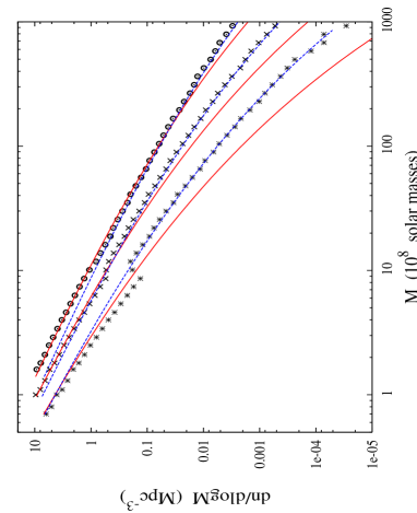
Figure 1: The halo mass function from our N-body simulation and merger history tree algorithm. The merger history tree generates all the halos below $10^{9}~{}M_{\odot}$, and the more massive halos derive from the N-body simulation. We plot curves for the merger tree plus resolved N-body halos at $z=6.5$ (circles), $8.7$ (x’s) and $11.1$ (asterisks). The solid curves are the Press-Schechter, and the dashed are the Sheth-Tormen mass functions for these redshifts. The low-mass cutoff for these curves is set by the HI atomic cooling mass $m_{\rm cool}$. The mass function of the merger tree halos agree well with the theoretical curves (especially at the lower two redshifts, which are the most relevant to this study).

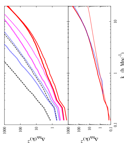
Figure 2: Top Panel: The mass-weighted halo power spectrum $\Delta_{hh}^{2}$ for $z=6.6$ (thin curves) and $11.1$ (thick curves) for several source models. [$\Delta_{hh}^{2}=k^{3}\langle\delta\rho_{h}(k)^{2}\rangle/(2\pi^{2})$, where $\delta\rho_{h}(k)$ is the fluctuation in the halo mass density in Fourier space.] The dot-dashed curves are for halos with $m>4\times 10^{10}~{}M_{\odot}$, the dashed are for the resolved halos with $m>2\times 10^{9}~{}M_{\odot}$, and the solid are for all halos above the cooling mass. We also include the power spectrum of halos above the cooling mass, but weighted as $m^{5/3}$ rather than $m$ (dotted curves) to match a source model discussed in §4. All halos with masses between the cooling mass and $10^{9}~{}M_{\odot}$ are incorporated with the merger tree method. Bottom Panel: The mass-weighted power spectrum of the source halos (merger tree + resolved halos) at $z=8.7$ (solid curve), and the power spectrum of a smaller box simulation ($20\;h^{-1}~{}{\rm Mpc}$, $1024^{3}$ particles) that resolves halos down to the cooling mass for $z=8.7$ (dotted curve). The power spectrum from the merger tree method agrees with this higher resolution run, boosting our confidence in this method. The thin solid curve is $k^{3}\,\bar{b}_{PS}^{2}\,P_{\delta\delta}(k,z)/2\pi^{2}$, in which $\bar{b}_{PS}$ is the average Press-Schechter bias and $P_{\delta\delta}$ is calculated using the Peacock and Dodds fitting formula.

The merger history tree algorithm generates the halos in Lagrangian space, requiring us to then map them to Eulerian space. The progenitor halos – the halos at the lowest redshift bin such that they sit on the top of a merger history tree – are generated within each coarse cell on a $64^{3}$ grid in Lagrangian space, and they are then randomly associated with one of the fine cells within its respective coarse cell (typically there are $256^{3}$ fine cells). This randomization is justified by the fact that Poisson fluctuations dominate over cosmological fluctuations at the scale of the coarse cell. To map our halos to Eulerian space in a self-consistent manner, we associate each progenitor halo with a particle whose initial (Lagrangian) position is the center of the same fine cell as the Lagrangian position of the halo. We then displace the particle at each redshift according to second order Lagrangian perturbation theory (Crocce et al. 2006). At higher redshifts, we split the progenitor halo into its daughter halos, and all daughter halos are associated with the same particle as their parent. This method for adding unresolved halos is similar to the PT halo algorithm, an algorithm to quickly generate mock galaxy surveys (Scoccimarro & Sheth 2002).

The bottom panel in Figure 2 plots the mass-weighted halo power spectrum $\Delta_{hh}^{2}$ at $z=8.7$ from a $1024^{3}$, $20~{}h^{-1}$ Mpc box simulation that resolves halos down to the cooling mass (dotted curve). Note that $\Delta_{hh}^{2}=k^{3}\langle\delta\rho_{h}(k)^{2}\rangle/(2\pi^{2})$, where $\delta\rho_{h}(k)$ is the fluctuation in the halo mass density in Fourier space. The $\Delta_{hh}^{2}$ of the merger history tree plus resolved halos (solid curve) agrees to better than $40\%$ at all scales with the small box $\Delta_{hh}^{2}$ (dotted curve). The level of agreement between the dotted and solid curves demonstrates that the merger tree method reliably incorporates the small mass halos in our simulations. The thin solid curve is an analytic prediction for the halo power spectrum given by $k^{3}\,\bar{b}_{PS}^{2}\,P_{\delta\delta}/(2\pi^{2})$, in which $P_{\delta\delta}$ is calculated using the Peacock and Dodds fitting formula for the density power spectrum, $\bar{b}_{PS}=\int_{m_{\rm cool}}^{\infty}dm\,m\,n_{PS}(m)\,b_{PS}(m)$, and $b_{PS}(m)$ is the Press-Schechter bias for a halo of mass $m$ [at $z=8.7$, $\bar{b}_{PS}=3.5$] (Mo & White 1996). This analytic estimate for $\Delta_{hh}^{2}$ ignores Poisson fluctuations, and a comparison with the other curves indicates that Poisson fluctuations are important on scales of $k\gtrsim 4\,h\;{\rm Mpc}^{-1}$.

The top panel in Figure 2 shows the mass-weighted power spectrum of halos above the cooling threshold from the merger history tree method (solid curves) and of the halos that are well resolved in our box with $m>2\times 10^{9}~{}M_{\odot}$ (dashed curves) at $z=6.6$ (thin curves) and $z=11.1$ (thick curves). The different spectrum of fluctuations between the solid and dashed curves suggests that incorporating the unresolved halos may lead to a different HII morphology. As the source halos become rarer, their spatial fluctuations increase and the Poisson component of the fluctuations becomes more important.

Table 1: Radiative transfer simulations discussed in this paper. Unless otherwise specified, the subgrid clumping factor $C_{\rm cell}$ is set to unity and the radiative transfer is performed on a $256^{3}$ grid. $M_{8}$ denotes the halo mass in units of $10^{8}~{}M_{\odot}$. The functions $C_{S2},~{}C_{S3}$ and $C_{S4}$ are calibrated such that the sources in the respective simulations output the same number of ionizing photons in each time step as the sources in simulation $S1$.

Simulation	Merger Tree Halos∗	$\dot{N}$ (photons s-1)	Comments
S1	yes	$2\times 10^{49}\,M_{8}$
S2	yes	$C_{S2}\,M_{8}^{1/3}$
S3	yes	$C_{S3}\,M_{8}^{5/3}$
S4	no	$C_{S4}\,M_{8}$	includes only $m>4\times 10^{10}~{}M_{\odot}$
F1	yes	$2\times 10^{49}\,M_{8}$	feedback on $m<M_{\rm J}/2$; $\tau_{SF}=100$ Myr
F2	yes	$2\times 10^{49}\,M_{8}$	feedback on $m<M_{\rm J}/2$; $\tau_{SF}=20$ Myr
F3	no	$2\times 10^{49}\,M_{8}$	includes only halos with $m>M_{\rm J}/2$
C1	no	$3\times 10^{49}\,M_{8}$	all cells set to mean density
C2	no	$3\times 10^{49}\,M_{8}$
C3	no	$3\times 10^{49}\,M_{8}$	$512^{3}$ grid
C4	no	$6\times 10^{49}\,M_{8}$	$C_{\rm cell}$ given by eqn. 4
C5	no	$6\times 10^{49}\,M_{8}$	$C_{\rm cell}=4+3\,\delta_{\rm cell}$
M1	no	$9\times 10^{49}\,M_{8}$
M2	no	$9\times 10^{49}\,M_{8}$	Iliev et al. (2005b) minihalos with $m_{\rm mini}>10^{5}M_{\odot}$
M3	no	$9\times 10^{49}\,M_{8}$	minihalos with $m_{\rm mini}>10^{5}M_{\odot}$, $\sigma_{\rm mh}=\pi r_{\rm vir}^{2}$
Z1	yes	$1\times 10^{50}\,M_{8}$
Z3	yes	$5\,C_{S3}\,M_{8}^{5/3}$

^∗ All radiative transfer simulations are post-processed on a density field that resolves halos down to $10^{9}\,M_{\odot}$. Halo mass resolution is extended beyond $10^{9}\,M_{\odot}$ with a merger tree. Here, ‘yes’ means the source halo resolution is supplemented with the merger tree down to $m_{\rm cool}$.

4 Sources

Now that we have a method for incorporating small mass halos into our simulations, we examine several prescriptions for populating the dark matter halos with ionizing sources. We consider models where POPII-like sources are responsible for the vast majority of the ionizing photons. Even among these sources, it is uncertain which galaxies will produce the ionizing photons. We consider four models for the source efficiencies. In all models, the ionizing luminosity $\dot{N}$ for a halo of mass $m$ is given by the relation $\dot{N}(m)=\alpha(m)\,m$. In simulation S1, the factor $\alpha$ is independent of halo mass. Simulation S2 uses the same source halos as S1 except $\alpha\propto m^{-2/3}$ (the lowest mass systems are the most efficient at converting gas into IGM ionizing photons). In simulation S3, we again use the same source halos but set $\alpha\propto m^{2/3}$ (the most massive systems are the most efficient). Finally, in simulation S4, $\alpha\propto m^{0}$, as in S1, except that only halos with $m>4\times 10^{10}~{}M_{\odot}$ are sources. At $z=9$, there are $500$ sources in S4 and, at $z=7$, there are $7000$ sources. These numbers are in contrast to the other simulations in this section in which there are over $1$ million sources at $z=9$ and over $3$ million at $z=7$.

Table 1 lists the parameters we use for the runs in this section. For simulation S1 we set $\dot{N}(m)=2\times 10^{49}\,m/(10^{8}\,M_{\odot})$ photons s^-1. To facilitate comparison, we normalized the photon production in the S2, S3 and S4 runs so that the same number of photons are outputted in each time step as in S1. In reality, as rarer sources dominate the ionizing budget, the rate at which the Universe is ionized quickens because the number of high mass halos is growing exponentially. Here we are interested in the structure of reionization, which is not significantly affected by the duration of this epoch.

The luminosity of our sources only depends on the halo mass. This parametrization is most reasonable if, once the gas has cooled within a halo, the timescale for its conversion into stars is at least comparable to the duration of reionization (or a few hundred million years). Springel & Hernquist (2003) measure a gas-to-star conversion timescale of over a gigayear in simulations of high redshift galaxies. However, many works in the literature parameterize star formation as proportional to the time derivative of the collapse fraction (e.g., Furlanetto et al. (2004b)). This parametrization assumes that the rate at which a galaxy converts its cold gas into stars is much shorter than the duration of reionization. The effects of alternative parameterizations of star formation on reionization are discussed at the end of this section.

The source prescriptions in S1, S2, S3 and S4 are all still reasonable in principle. The least massive systems could dominate the budget of ionizing photons because it may be easier for ionizing photons to escape from the smallest mass halos. Wood & Loeb (2000) find that this is the case in static halos owing to the shallower potential well of the low mass halos. Internal feedback from galactic winds and supernova bubbles may further enhance the escaping luminosity of smaller halos relative to the more massive halos. Internal feedback can also act to shut off star formation. Springel & Hernquist (2003) find that feedback from galactic winds suppresses star formation in the least massive systems relative to the more massive. The scaling $\alpha\sim m^{2/3}$ taken in model S3 is motivated by the observed star formation efficiency in low redshift dwarf galaxies (Kauffmann et al. 2003).

Because star formation is a complicated process, observations rather than theory will likely drive our knowledge of the high redshift sources. From present observational constraints, the source prescription used in S4 is closest to being ruled out: There is mounting evidence that the highest mass halos cannot produce enough photons to ionize the Universe (Stark et al. 2006).

All the simulations in this section were performed on a $256^{3}$ grid, and the subgrid clumping factor is set to unity (i.e., density fluctuations on scales smaller than the cell scale are ignored). In subsequent sections, we increase the level of clumping and include dense absorbing systems that limit the mean free path of photons. Due to the lack of gas clumping in the runs in this section, our simulations underestimate the number of ionizing photons needed to reionize the IGM. However, we find that neither the dense absorbers nor the increased clumping have a substantial effect on the topology of the bubbles for fixed $\bar{x}_{i}$, except in extreme scenarios or at higher ionization fractions than we consider.

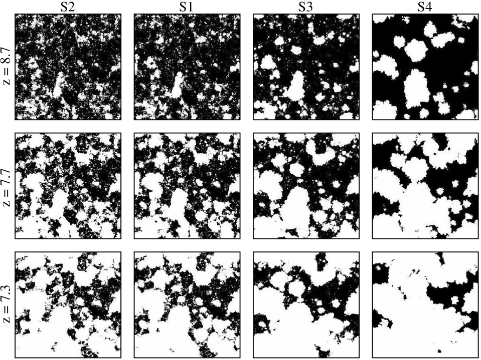
Figure 3: Comparison of four radiative transfer simulations post-processed on the same density field, but using different source prescriptions parameterized by $\dot{N}(m)=\alpha(m)\,m$. The white regions are ionized and the black are neutral. The left, left-center, right-center and right panels are respectively cuts through simulations S2 ($\alpha\propto m^{-2/3}$), S1 ($\alpha\propto m^{0}$), S3 ($\alpha\propto m^{2/3}$), and S4 ($\alpha\propto m^{0}$, but only halos with $m>4\times 10^{10}\,M_{\odot}$ host sources). For the top panels, the volume ionized fraction is $\bar{x}_{i,V}\approx 0.2$ (the mass ionized fraction is $\bar{x}_{i,M}\approx 0.3$) and $z=8.7$. For the middle panels, $\bar{x}_{i,V}\approx 0.5$ ($x_{i,M}\approx 0.6$) and $z=7.7$, and for the bottom panels, $\bar{x}_{i,V}\approx 0.7$ ($\bar{x}_{i,M}\approx 0.8$) and $z=7.3$. Note that the S4 simulation outputs have the same $\bar{x}_{i,M}$, but $\bar{x}_{i,V}$ that are typically $0.1$ smaller than that of other runs. In S4 the source fluctuations are nearly Poissonian, resulting in the bubbles being uncorrelated with the density field ($\bar{x}_{i,V}\approx\bar{x}_{i,M}$). Each panel is $94~{}{\rm Mpc}$ wide and would subtend $0.6$ degrees on the sky.

Figure 3 compares slices through the ionization field from the S2, S1, S3, and S4 simulations (left to right) at redshifts $8.7,7.7$ and $7.3$ (top, middle and bottom panels). Panels in a row have the same mass ionized fraction $\bar{x}_{i,M}$. All panels have bubbles located around the large-scale overdense regions, but the bubbles better trace the overdensities as the less massive sources dominate. Reionization in both S1 and S2 is dominated by the low mass sources and results in a nearly identical reionization morphology when comparing at fixed $\bar{x}_{i}$. The HII regions in S3 are larger and more spherical than they are in S1 and S2. The bubbles are still larger in S4.

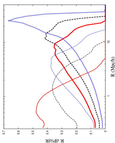
Figure 4: The volume-weighted bubble radius PDF for the S1 (solid curves), S3 (dot-dashed curves), and S4 (dotted curves) simulations. See the text for our definition of the bubble radius $R$. We do not include curves for the S2 simulation because they are similar to those for S1. The thin curves are at $z=8.7$ and $\bar{x}_{i,M}=0.3$, and the thick curves are at $z=7.3$ and $\bar{x}_{i,M}=0.8$. Simulation S4 has the rarest sources and the largest HII regions of the four models.

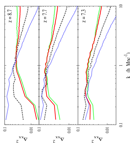
Figure 5: The ionization fraction power spectrum $\Delta_{xx}(k)^{2}=k^{3}P_{xx}(k)/2\pi^{2}$ for the S1 (solid curves), S2 (dashed curves), S3 (dot-dashed curves) and S4 (dotted curves) simulations. For the top panels, $\bar{x}_{i,V}\approx 0.2$ ($\bar{x}_{i,M}\approx 0.3$), for the middle panels, $\bar{x}_{i,V}\approx 0.5$ ($x_{i,M}\approx 0.6$), and for the bottom panels, $\bar{x}_{i,V}\approx 0.7$ ($\bar{x}_{i,M}\approx 0.8$). In all panels, the fluctuations are larger at $k\lesssim 1~{}h\,{\rm Mpc}^{-1}$ in S3 and S4 than they are in S1 and S2. As the most massive halos contribute more of the ionizing photons, the ionization fraction fluctuations increase at large scales.

The differences between the ionization maps owe to the bias differences between the sources. As the sources become more biased, they become more clustered around the densest regions, resulting in the bubbles becoming larger. In Press-Schechter theory, the luminosity-weighted average bias at $z=8$ is $\bar{b}_{\rm PS}=2.8$ for the S2 source prescription, $3.2$ for the S1, $5.0$ for the S3, and $7.3$ for the S4. The S4 sources are located in the highest density peaks in the Universe and the fluctuations in the density of these sources is the largest. [See respectively, the thin solid, thin dotted, and thin dash-dotted lines in Fig. 2 for a comparison of the luminosity-weighted power spectra for the S1, S3, and S4 sources at $z=6.6$.] The differences between the ionization maps for S1, S3, and S4 should allow observations to distinguish between these scenarios (as discussed in §8).

This trend of bubble size increasing with average source mass was predicted in the analytic work of Furlanetto et al. (2005). Analytic models typically ignore Poisson fluctuations in the source abundance, which can dominate over cosmological fluctuations when relatively massive sources dominate the photon production. For example, the bubble scale in S4 is roughly $20$ Mpc at $z=7.7$ and $\bar{x}_{i}=0.5$ – a scale where Poisson fluctuations dominate over the cosmological ones. For the S1 and S2 source models, cosmological fluctuations dominate over Poisson fluctuations on the scale of a typical bubble, but Poisson fluctuations can be important in smaller bubbles. This deficiency of analytic models was noted in Zahn et al. (2006b).

Figure 4 plots the bubble size distribution from S1 (solid curves), S3 (dot-dashed curves), and S4 (dotted curves) at $\bar{x}_{i,M}=0.3$ (thin curves) and $\bar{x}_{i,M}=0.8$ (thick curves). The S2 simulation is not included here; it yields bubble sizes that are similar to those in S1. How do we define the bubble “radius” since the bubbles are far from spherical? For each cell in the box, we find the largest sphere centered around this cell that is $90\%$ ionized. We say that each cell is in a bubble of size equal to the radius of this sphere. We then tabulate the radius from all the ionized cells to calculate the volume-weighted bubble PDF (zero-radius bubbles are not included in the tabulation). This definition of bubble size is chosen to facilitate comparison with analytic models of reionization based on the excursion set formalism in which the bubble radius is similarly defined (Furlanetto et al. 2004b). The bubbles are largest in S4 and smallest in S1, and in all runs there is a characteristic bubble radius.

It is useful to compare the measured bubble size distribution to the size distribution predicted in analytic models. The “log-normal” distribution of bubbles found in analytic models is present in these simulations. The bubble size distribution becomes more sharply peaked in $\log(R)$ with increasing $\bar{x}_{i}$ in our simulations, a trend that was predicted by analytic models (Furlanetto et al. 2005). A more detailed comparison of the bubble sizes between these simulations and analytic models is given in Zahn et al. (2006b).

Figure 5 plots the dimensionless ionization fraction power spectrum $\Delta_{xx}^{2}$ for the four simulations (S1 – solid, S2 – dashed, S3 – dot–dashed, S4 – dotted) for the volume ionized fractions $\bar{x}_{i,V}\approx 0.2$ (top panel), $\bar{x}_{i,V}\approx 0.5$ (middle panel) and $\bar{x}_{i,V}\approx 0.7$ (bottom panel). [The $\bar{x}_{i,V}$ for S4 is $\approx 0.1$ smaller than these values.] Note that $\Delta_{xx}(k)^{2}=k^{3}\,P_{xx}(k)/(2\pi^{2})$ in which $(2\pi)^{3}\,P_{xx}(k)\,\delta_{D}({\bf k}-{\bf k}^{\prime})=\langle x_{i}({\bf k})x_{i}({\bf k}^{\prime})\rangle$. For some $\Delta_{xx}^{2}$ the power peaks at the box scale ($k\approx 0.1~{}{\rm Mpc}^{-1}$), particularly at larger $\bar{x}_{i}$. This indicates that there is substantial power in ionization fraction fluctuations on scales larger than our simulation box in some of the considered models. Therefore, the box we use is too small to make statistical predictions about reionization for some of the models and at some $\bar{x}_{i}$. Lyman-limit systems or minihalos may reduce the size of the largest bubbles and alleviate this difficulty (see §6.2).

It is useful to note that an ionization field that is composed of fully neutral and ionized regions with total ionized fraction $\bar{x}_{i,V}$ has variance of $\bar{x}_{i,V}-\bar{x}_{i,V}^{2}$ on small scales, implying that

$$\int_{0}^{\infty}d\log k~{}\Delta_{xx}(k)^{2}=\bar{x}_{i,V}-\bar{x}_{i,V}^{2}.$$ (3)

Because of equation (3) and because the snapshot from S4 has more power on large scales, the snapshots from S1, S2, and S3 must have more power than S4 on small scales for the same $\bar{x}_{i}$. The distribution of power has important implications for upcoming observations. Generally speaking, the more power on large scales ($k<1\,h\;{\rm Mpc}^{-1}$), the more observable the signal (see §8).

The picture of reionization seen in simulations S1, S2 and S3 is different from that seen in the simulations of Iliev et al. (2006a). Their simulations resolve halos with $m>2\times 10^{9}\;M_{\odot}$, and reionization ends at $z\approx 12$ in their calculations. Hence, the resolved halos in their simulations are very rare and, of the four source models we consider, are most similar in abundance to the source halos in S4. Their reionization snapshots give the visual impression of many overlapping spheres. We do see, particularly in simulation S4, that the bubbles become more spherical as the sources become rarer. See Zahn et al. (2006b) for further comparison.

The prescription we use for the luminosity of the sources is simplistic. In all of our source models, the luminosity of a halo is monotonic in the halo mass such that the characteristic source mass is either $m_{\rm cool}$ or $m_{*}$ – the halo mass that characterizes the transition to the exponential tail in the luminosity function. Star formation is complicated, and the characteristic mass of a source could be an intermediate mass between $m_{\rm cool}$ and $m_{*}$. In this case, the bias of the sources will fall between the source bias in S2 and in S3, and, therefore, the bubbles sizes will be between the sizes in S2 and in S3 if we compare at fixed $\bar{x}_{i}$.

Surely the luminosity of galaxies depends on additional parameters besides the halo mass. Other studies have parameterized the luminosity of the sources as proportional to the time derivative of the collapse fraction, considering the accretion of gas onto sources as a better proxy for the star formation rate than the gas mass of the sources. We have run simulations with the luminosity proportional to the time derivative of the collapse fraction in a cell. We find that the morphology of reionization is very similar between this parameterization and that of the constant mass-to-light model. The reason for this similarity is that the collapse fraction in a given region is changing nearly exponentially with time and so the rate of halo mass growth is proportional to the halo mass. Alternatively, star formation or quasar activity may be correlated with major mergers (see Hopkins et al. 2006a,b, Li et al. 2006 for discussion). Since major merger events are more biased, this results in larger bubbles. Cohn & Chang (2006) used an analytic model to derive the bubble sizes in merger-driven scenarios. In addition, it might have been possible for the gas in smaller mass galaxies ($m\gtrsim 10^{5}~{}M_{\odot}$) to cool via $H_{2}$ transitions. If this is the case, stars would form in halos with smaller masses than are considered here. These sources would be less biased, and, therefore, the HII regions would be smaller and more fragmented.

5 Source Suppression from Photo-heating

The extent to which photo-heating from a passing ionization front affects the ionizing sources and, as a result, the reionization process is not well understood. Often, when included in a study, the effect of photo-heating is parameterized in a simplistic fashion: Star formation is assumed to be completely shut off in the low mass sources as soon as an ionizing front has passed. However, sources that form prior to a front passing will have a cool reservoir of gas with which to make stars. Since photo-heating can suppress subsequent accretion onto these objects, eventually this reservoir will run dry and all the gas will have been converted to stars. The timescale over which this reservoir will be depleted is uncertain (see discussion in §4).

Furthermore, the mass threshold at which sources will be suppressed by photo-heating is fairly unconstrained. Often the suppression mass scale is taken to be the linear theory Jeans mass $M_{\rm J}$. This choice is, however, problematic. The gas will not instantaneously respond to photo-heating – there will be some delay, leading to a time dependent suppression threshold that only asymptotically approaches the Jeans mass for linear fluctuations (Gnedin & Hui 1998). In addition, a spherical perturbation that collapses at $z=8.0$ was at turnaround at $z=13.3$. An ionization front passing this collapsing mass at, say, $z=9$, will do little to prevent the gas from cooling. The collapsing gas is already significantly overdense prior to front-crossing, giving it a large collisional cooling rate and possibly allowing it to self shield (Dijkstra et al. 2004). Dijkstra et al. (2004) finds in 1-D simulations that a substantial fraction of collapsing density peaks with mass below the Jeans mass threshold (or $2.7\times 10^{9}~{}M_{\odot}$ at $z=7$ for $T_{\rm gas}=10^{4}$ K) are still able to collapse and form gas-rich halos in ionized regions, and Kitayama et al. (2000) and Kitayama et al. (2001) find an even larger fraction than Dijkstra et al. (2004) in 3-D simulations.

Iliev et al. (2006c) was the first to investigate with large-scale simulations of reionization the effect feedback on the sources from photo-heating has on reionization. They applied the rather extreme criterion that star formation in all halos below $10^{9}~{}M_{\odot}$ is shut off after $20$ million years in ionized regions. They concluded from this study that the small halos do not play an important role in ionizing the IGM. Here we expand upon the work of Iliev et al. (2006c) to include more general parameterizations for the feedback from photo-heating.

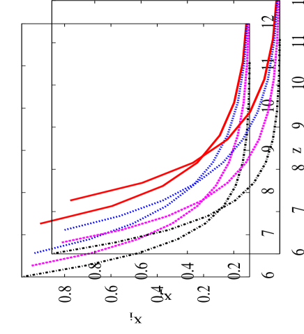
Figure 6: The impact of thermal feedback on the ionization history. The ionization history $\bar{x}_{i,V}(z)$ for the S1 (solid curve), F1 (dotted curve), F2 (dashed curve), and F3 (dot-dashed curve) simulations. Simulation S1 has no feedback, and F3 has maximal feedback. Feedback extends the duration of reionization by as much as $200$ Myr in our simulations.

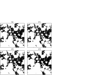
Figure 7: The impact of thermal feedback on the morphology of reionization. Slices through snapshots in which $\bar{x}_{i,V}\approx 0.7$. The white regions are ionized and the black are neutral. S1 includes no thermal feedback, F1 has minimal feedback with $\tau_{SF}=100$ Myr, F2 has strong feedback with $\tau_{SF}=20$ Myr, and F3 uses only halos with $m>M_{\rm J}/2$ as the sources (or, equivalently, $\tau_{SF}=0$). Notice that even the ionization maps from S1 and F3 do not differ by much, which shows that feedback has a small effect on the structure of reionization.

The parameterizations we adopt for source suppression owing to photo-heating are simplistic. However, we show that the structure of reionization is largely unaffected by feedback even for an aggressive parametrization of suppression. If an ionizing front passes a source with luminosity $L_{0}$ at time $t_{i}$ then at time $t$ we set its luminosity to be $L(t)=L_{0}\,\exp[-(t-t_{i})/\tau_{SF}]$, where $\tau_{SF}$ can be thought of as the timescale over which the cool gas in the potential well of a source is converted into stars. We set $\tau_{SF}=100,~{}20$ and $0$ million years in simulations F1, F2, and F3, respectively. We assume that this luminosity suppression affects halos with masses below $M_{\rm J}/2$, where $M_{\rm J}$ is calculated for gas at $T=10^{4}\,K$ (or $1.4\times 10^{9}~{}M_{\odot}$ at $z=7$). This fixed suppression mass misses the time dependent response of the gas to photo-heating. The suppression mass $M_{\rm J}/2$ is approximately the suppression mass found at $z=7$ in Dijkstra et al. (2004). This suppression mass is an order of magnitude larger than that found by Kitayama et al. (2000). Furthermore, we assume that halos that form in already ionized regions with masses below $M_{\rm J}/2$ have zero star formation and do not contribute to reionization.

First, in agreement with previous studies, we note that thermal feedback can delay and extend the reionization process (Fig. 6). Simulation S1 (solid curve) does not include feedback, whereas simulation F3 (dot-dashed) includes maximal feedback ($\tau_{SF}=0$). The duration of reionization is extended by about $200$ million years in this case. For the other feedback scenarios (F1 and F2), reionization is extended by a shorter period ($100$ and $150$ million years).

Figure 7 displays slices through snapshots with $\bar{x}_{i,V}=0.7$ for the simulations S1, F1, F2, and F3. In S1, halos below the $m_{\rm cool}$ always contribute ionizing photons, whereas in simulation F3 only halos above $M_{\rm J}/2$ contribute. The differences between S1 and F3 are minor: The small mass sources do not change the structure of reionization significantly. S1 has more small bubbles, and the HII fronts have more small-scale features. Simulation F1 ($\tau_{SF}=100$ Myr) is most similar to S1 – long gas-to-star formation timescales essentially negate the effect of feedback, and simulation F2 ($\tau_{SF}=20$ Myr) has less structure in the voids than F1. In conclusion, simulations S1 and F1–3 have a very similar morphology at fixed $\bar{x}_{i}$. Feedback does not significantly affect the structure of reionization. We find that this conclusion still holds if we compare at other $\bar{x}_{i,V}$ as well.

To make the comparison of feedback models more quantitative, we contrast the $\Delta_{xx}$ at $\bar{x}_{i}=0.7$ for these four models. We find that the $\Delta_{xx}$ of the S1, F1, and F2 models agree to approximately $10\%$ at all scales and that the $\Delta_{xx}$ of the S1 and F3 models (no feedback and maximal feedback models) differ by at most $20\%$, with the largest differences being for modes near the box scale and for modes with $k>5\,h\;{\rm Mpc}^{-1}$.

It is simple to understand why thermal feedback has little impact on the size distribution and morphology of HII regions (provided we compare at fixed $\bar{x}_{i}$). The bubble size distribution and morphology are mainly sensitive to the bias of the ionizing source host halos and to Poisson fluctuations in the halo abundance for sufficiently rare source halos. The top panel in Figure 2 compares the luminosity-weighted halo power spectrum $\Delta_{hh}^{2}$ for halos above the cooling mass at $z=6.6$ (thin, solid curve) compared to $\Delta_{hh}^{2}$ for halos with $m>2\times 10^{9}~{}M_{\odot}$ (thin, dashed curve). Notice that the difference between these curves is less than the difference between, for example, these curves and those for the S3 sources (thin, dotted curve). In terms of the Press-Schechter bias at $z=8$, $\bar{b}_{\rm PS}=3.2$ for the S1 sources whereas $\bar{b}_{\rm PS}=4.3$ for halos with $m>M_{\rm J}/2=1.4\times 10^{9}~{}M_{\odot}$. These values should be contrasted with $\bar{b}_{\rm PS}=5.0$ for the S3 sources and $\bar{b}_{\rm PS}=7.3$ for the S4 sources. Therefore, if halos with $m\lesssim 1.4\times 10^{9}~{}M_{\odot}$ are evaporated (as in this section), the morphology of reionization is not changed as substantially as the difference between the morphology in the S1 and in the S3/S4 simulations. In fact, Figure 7 shows that the bubbles are largely unchanged by feedback.

All simulations in this section are parameterized such that $\dot{N}\propto m$ and such that the suppression scale is $M_{\rm J}/2$. For lower $\bar{x}_{i,V}$ than are shown in Figure 7, the effect of feedback in our simulations is even less significant. If the highest mass sources are more efficient at producing ionizing photons, reionization will be extended by a smaller amount by feedback than we find, whereas if the low mass sources are more efficient, feedback will extend reionization by a larger amount. The conclusion that the structure of reionization is only modestly affected by feedback holds even if the sources near $m_{\rm cool}$ are more efficient at producing ionizing photons then we have assumed: We found in §4 that as we made the low mass sources more efficient, the properties of the HII regions are essentially unchanged (compare the panels from S1 and S2 in Fig. 3). Lastly, we believe that our choice of $M_{\rm J}/2$ is a fairly extreme suppression mass for low redshift, POPII star reionization scenarios owing to effects mentioned at the beginning of this section. If the suppression mass is larger than $M_{\rm J}/2$ or if reionization happens at a higher redshift but with the same suppression mass, thermal feedback will be more important. However, at $z>10$ both Dijkstra et al. (2004) and Kitayama et al. (2000) find that the suppression mass is much lower than $10^{9}~{}M_{\odot}$ .

If molecular hydrogen cooling is able to cool the gas in a halo to form a galaxy then most star formation could take place in halos with $m\ll m_{\rm cool}$. In such a case, thermal feedback could play a more important role in shaping the structure of reionization. Kramer et al. (2006) found that this scenario could lead to a bimodal bubble size distribution. (Note that in the models that we consider in which only halos with $m>m_{\rm cool}$ form stars, feedback does not create a bimodal bubble size distribution, and the size distribution of the bubbles is largely unchanged by thermal feedback.)

6 Effect of Density Inhomogeneities

Density inhomogeneities potentially play an important role in shaping the HII regions during reionization. On small scales, density inhomogeneities lead to the outside-in reionization observed in the simulations of Gnedin (2000a). The role of these inhomogeneities on the large-scale bubble morphology has not been investigated in detailed simulations. Analytic models make simplistic assumptions to incorporate their effects. These models spherically average the density fluctuations in a bubble and typically treat a higher level of recombinations as equivalent to decreasing the ionizing efficiency of the sources.

Previous large-scale radiative transfer simulations of reionization either ignored subgrid density inhomogeneities entirely, or they calibrated their subgrid clumping factor from smaller simulations (Mellema et al. 2006; Kohler et al. 2005). A simulation of Mellema et al. (2006) uses a clumping factor that is independent of $\delta$ and $\bar{x}_{i}$ and neither the simulations of Mellema et al. (2006) nor Kohler et al. (2005) include a dispersion in the clumping for a cell of a given overdensity. Both studies of clumping also assume that the clumping factor is independent of the local reheating and ionization history, which is incorrect in detail. In linear theory, the smallest gas clump – which is intimately tied to the gas clumping factor – is given by the filtering mass $M_{f}$ (Gnedin & Hui 1998), and this mass incorporates the time-dependent gas response to heating (see §C). The filtering mass provides some framework to understand the small-scale gas clumping. It is important to understand how sensitive the characteristics of reionization are to gas clumping – to what extent can gas clumping be ignored or included in only a primitive manner?

Minihalos – virialized objects with $T_{\rm vir}<10^{4}$ K – contribute to the clumping differently than does the diffuse IGM. These virialized objects are unresolved in all current large-scale reionization simulations. Minihalos are extremely dense and act as opaque absorbers until they are photo-evaporated. Since the inner regions of minihalos are self-shielded, it is difficult to describe the effect of minihalos with a subgrid clumping factor. In addition, most photons that pass through a cell should not be affected by a minihalo because the mean free path for a ray to intersect a minihalo can range between $1$ and $100$ Mpc. Absorptions by minihalos are unimportant when the HII regions are much smaller than the mean free path. Once the bubble size becomes comparable to the mean free path, minihalos may be the dominant sinks of ionizing photons within a bubble. Furlanetto & Oh (2005) predict that minihalos create a sharp large-scale cutoff in the size distribution of bubbles, particularly when the Universe is largely ionized. If this prediction is true, large scale topological features during reionization can be used to probe small-scale density fluctuations.

We split the discussion in this section into two components: (1) quasi-linear IGM density inhomogeneities, and (2) the minihalos. (Our discussion on the effect of minihalos also applies to the effect of a more general class of dense absorbers, Lyman-limit systems.) The technology needed to describe these two forms of gas clumping is quite different. In this section, we use only the halos that are well resolved in the simulation as our sources ($m>2\times 10^{9}~{}M_{\odot}$), and we set the luminosity proportional to the halo mass. While this source prescription is probably unrealistic, we found in §5 that including less massive halos does not change considerably the structure of reionization.

6.1 IGM clumping

We cannot realistically calculate the clumpiness of the gas from the N-body simulation used in this paper. In order to investigate the effect of the clumping, we consider four toy models for clumping of the IGM. Simulation C1 uses a $256^{3}$ grid, setting the baryonic overdensity to zero and the subgrid clumping factor $C_{\rm cell}$ to unity in every cell. In other words, the IGM is completely homogeneous in this model. Simulation C2 is a $256^{3}$ simulation also with $C_{\rm cell}=1$, but it uses the gridded N-body density field. The cell mass in C2 is $2\times 10^{9}~{}M_{\odot}$, approximately the Jeans mass for $10^{4}$ K gas at $z=6$. Simulation C3 is a $512^{3}$ simulation with $C_{\rm cell}=1$. The cell mass in C3 is $3\times 10^{8}~{}M_{\odot}$, below the Jeans mass at relevant redshifts, but possibly above the filtering mass. Table 1 lists the specifications used in the C1–4 simulations.

When the Universe becomes reionized, the filtering mass $M_{f}$ can be orders of magnitude smaller than the Jeans mass. It takes hundreds of millions of years for the gas to respond fully to the photo-heating and clump at the limiting scale. Therefore, the $512^{3}$ run is closer to reality than the $256^{3}$ one, but still underestimates the effect of clumping on the IGM. To account for this higher degree of clumping, we run simulation C4. This is a $256^{3}$ simulation with twice the ionizing efficiency of the other runs such that overlap occurs at around the same time. In addition, we set the subgrid clumping factor in C4 to

$$C_{\rm cell} = 1+\frac{\rho_{0}^{2}}{\rho_{\rm cell}^{2}}\,\int_{0}^{\infty}\,\frac{k^{2}dk}{2\pi^{2}}\,\left[1-W^{2}_{{\rm cell}}(k)\right]\,P_{\delta\delta}(k,z)$$ (4)

$$\times \exp(-k^{2}/(k_{f}^{-1}+k_{5}^{-1})^{-2}),$$

where $k_{f}$ is the scale that contains the mass $M_{f}$ (which is given by equation 9), $W_{{\rm cell}}$ is the cell window function, and $k_{5}$ is the wavevector that corresponds to $10^{5}~{}M_{\odot}$ at the mean density – the minimum mass baryonic clump that we allow, consistent with a minimal amount of reheating. For simplicity, we use a spherical top hat in real space that has the same volume as a grid cell for $W_{{\rm cell}}$. We use the Peacock and Dodds power spectrum for $P_{\delta\delta}(k,z)$. The filtering mass $M_{f}$ depends on the redshift at which the cell was ionized. Once a region is ionized, this mass increases with time and $C_{\rm cell}$ typically decreases.

Equation (4) would be correct if the window function of a cell were instead a top hat in $k$-space, if mode coupling were absent between modes smaller and larger than the cell scale, and if the quantity $M_{f}$ were appropriate outside of linear theory (there is evidence that it is appropriate [§C]). Since we are considering non-linear scales, mode coupling is important and tends to make the more massive cells have higher clumping factors than equation (4) predicts. In the limit in which most of the density fluctuations are at scales smaller than the cell, equation (4) predicts that the number of recombinations ($\propto C_{\rm cell}\,\rho_{\rm cell}\,\rho_{\rm cell}$) is independent of the cell’s density. This prediction is probably unphysical.

Note that we assume that the gas clumping in a cell is independent of the cell’s ionization fraction in all of the simulations. This assumption is justified for the gas in the diffuse IGM because this low density gas stays almost fully ionized when an ionization front passes, provided that there is an ionizing background. Virialized objects, such as minihalos, in which the local ionized fraction can be a function of density, are included in the computation in §6.2.

The reionization scenarios in this section reach $\bar{x}_{i}=0.5$ near $z=7$. The reionization epoch in simulation C4 is slightly more extended than the other scenarios owing to an enhanced number of recombinations. The volume-averaged clumping factor in ionized regions $C_{V}$ is $30$ at $z=7$ in C4, whereas it is $1.6$ in C2 and it is $2.7$ in C3. The total number of IGM photons that escape into the IGM per ionized baryon is $3$ in C4 at the end of reionization, whereas it is between $1.2-1.3$ in C2 and C3. (The recombination rate is proportional to the clumping factor.) Note that we have removed the particles that are associated with halos from the density grid in these simulations since most absorptions within these halos are already encapsulated in the factor $f_{\rm esc}$. Other studies left the halos in the density field (Gnedin 2000a; Ciardi et al. 2003), yielding a large number of recombinations within the source cells (which can be at hundreds of times the mean density) and therefore a larger photon to ionized baryon ratio.

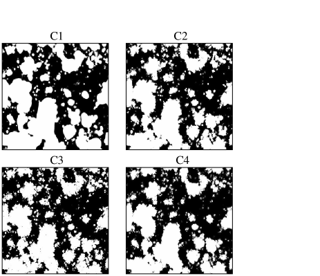
Figure 8: The impact of gas clumping on the structure of reionization. A slice through the C1 (top left), C2 (top right), C3 (bottom left) and C4 (bottom right) runs at $z\approx 7$ and $\bar{x}_{i}\approx 0.5$. All the cells in C1 are at the the mean density. Simulation C2 is run on top of the N-body simulation density field gridded to $256^{3}$, and C3 is the same but gridded to $512^{3}$. Simulations C1, C2, and C3 set $C_{\rm cell}=1$. Simulation C4 uses the $256^{3}$ grid with equation (4) for $C_{\rm cell}$. The additional clumpiness in C2-C4 over C1 adds structure to the ionization front. Simulation C4 has at least $10\times$ more recombinations than in the other runs.

Figure 8 depicts a slice through the box at $\bar{x}_{i,V}\approx 0.5$ for the C1, C2, C3 and C4 simulations. The ionization field in the top left panel (a snapshot from simulation C1, which uses a homogeneous density field) has less structure on the bubble edges than in the other runs. The picture seen in the top left panel is the most similar of all the panels to the picture of reionization seen in Monte-Carlo realizations of HII regions using the Furlanetto et al. (2004b) analytic model (see figures in Zahn et al. (2006b)). This model spherically averages the density field around a cell to determine its ionization fraction, washing out much of the small-scale structure in the density field. The $256^{3}$ and $512^{3}$ runs have a similar morphology despite the $512^{3}$ run’s higher resolution and larger volume-averaged clumping factor. When we boost the subgrid clumping factor substantially for the C4 run, this action does not significantly change the morphology, even though this simulation has a factor of $10$ more recombinations than the C2 and C3 simulations.

The $\Delta_{xx}^{2}$ for the C1–4 runs at $\bar{x}_{i,V}\approx 0.5$ agree to better than $20\%$ at scales larger than a Mpc. Simulation C1 has the least power of all the runs at megaparsec scales because it is missing the density-induced structure at the bubble edges. In conclusion, the differences in power from clumping in the considered models are minor compared to the differences that arise owing to the different source prescriptions.

In the C4 run, the subgrid clumping factor decreases as a function of the cell’s density (eqn. 4). We know that overdense regions form substantially more structure, and, therefore, it is possible that the subgrid clumping factor actually increases with density. To test whether such a prescription for clumpiness alters the morphology of reionization, we ran a small-scale clumping run C5 with $C_{\rm cell}=4+3\,\delta_{C}$, in which $\delta_{C}$ is the baryonic overdensity smoothed at the cell scale. This clumping prescription yields a similar scaling with density to the $C_{\rm cell}\sim\rho_{\rm cell}^{0.86}$ that Kohler et al. (2005) finds in a $4~{}h^{-1}~{}{\rm Mpc}$ simulation in which the halo particles are also removed from the density field. This parametrization results in a photon to ionized baryon ratio of $\approx 2$ at the end of reionization and $C_{V}\approx 20$ throughout reionization. We do not plot the results for C5, but we find that the HII regions have slightly more structure on the edges in this case than in C3 and C4. Overall, the structure of reionization is not significantly altered in C5 from the other clumping runs.

Why does clumping not affect the large-scale morphology of reionization? Qualitatively, large-scale density fluctuations significantly enhance the mass in sources that are present within an overdense region relative to the mean. However, the number of absorptions and recombinations per unit volume are not enhanced by the same margin. This leads to the enhanced abundance of ionizing photons winning in overdense regions and shaping the morphology of reionization. For a more quantitative treatment, one can solve for the overdensity that a region must have to be ionized given some source prescription and parametrization of the gas clumping. This overdensity threshold can then be used to calculate the bubble size distribution with the excursion set formalism (Furlanetto et al. 2004b; Bond et al. 1991). For reasonable parameterizations of the clumping factor, this exercise shows that clumping does not significantly change the bubble morphology for fixed $\bar{x}_{i}$ (McQuinn 2006).

On smaller scales, density fluctuations become more important in shaping reionization. For a single HII region ionizing a region of $10~{}{\rm Mpc}$ in radius at $z=7$, the HII region is not a perfect sphere, but has fluctuations in radius with $\Delta R/R\approx 0.2$. These fluctuations are generated by column density fluctuations between different lines from the source to the bubble edges. Lines with lower column densities will lead to fingers protruding from the HII regions. Such features are also present when many sources are within a bubble.

In addition to imprinting structure on the bubble edges, clumpiness has a considerable effect on the part in $10^{4}$ fluctuations in the neutral fraction within the bubbles. We will come back to this in future work.

In conclusion, quasi-linear density fluctuations imprint substructure on the bubble edges, but do not affect the large-scale morphology of the bubbles. Quasi-linear fluctuations also increase the number of recombinations and can extend reionization. We address the effect of self-shielding, non-linear density enhancements in §6.2.

6.2 Minihalos

The minimum mass minihalo that retains gas depends on the thermal history of the IGM. The Jeans mass at $z=10$ for gas that cools adiabatically since thermal decoupling from the CMB is $6\times 10^{3}~{}M_{\odot}$ (Barkana & Loeb 2002) and the filtering mass is approximately ten times larger (Gnedin & Hui 1998). However, reheating by X-rays prior to reionization will make the gas warmer than this, erasing gas density fluctuations at progressively larger scales. Furlanetto (2006) estimates that if POPII stars are responsible for reionization then the gas temperature is a couple hundred degrees Kelvin prior to the time the Universe is $10\%$ ionized. This estimate is based on extrapolating local X-ray luminosities to high redshifts. A heated, neutral IGM has a Jeans mass of $M_{\rm J}=4\times 10^{6}~{}M_{\odot}\,[{T}/(200\,{\rm K})\times(1+z)/(10)]^{3/2}$.

An isolated minihalo that holds onto its gas during reheating will subsequently lose its gas via photo-evaporation as ionizing flux impinges upon it (Barkana & Loeb 1999; Shapiro et al. 2004). The timescale for photo-evaporation $t_{\rm ev}$ of a minihalo is roughly the sound-crossing time of the halo, which for $10^{4}$ K gas ionized is (Shapiro et al. 2004)

$$t_{\rm ev}=100\,{\rm Myr}~{}\left(\frac{M}{10^{7}\,M_{\odot}}\right)^{1/3}\,\left(\frac{10}{1+z}\right).$$ (5)

This formula works well when the incident flux is large, but under-predicts the evaporation time for the ionizing fluxes that are typical during reionization (Iliev et al. 2005b). The duration of reionization in our simulations is a few hundred million years, comparable to the evaporation timescale of minihalos (eqn. 5), suggesting that minihalos will be present for all times during reionization.

Prior to evaporation, a minihalo is optically thick for a typical ionizing photon. An incident photon ionizes a hydrogen atom within the minihalo and the photon’s energy is converted primarily into kinetic energy of the minihalo gas rather than into additional IGM ionizing photons. The mean free path at $z=6$ to intersect a halo of mass $(10^{5},10^{6},10^{7})$ $M_{\odot}$ within a virial radius is $(4,7,17)~{}{\rm Mpc}$ [or at $z=12$ is $(6,19,74)~{}{\rm Mpc}$] if we assume the Press-Schechter mass function.

Several previous calculations have attempted to encapsulate the effect of minihalos via a clumping factor (e.g., Haiman et al. 2000). We emphasize that this is not an appropriate way to treat minihalos. Minihalos are self-shielded such that the densest inner regions should not contribute to the clumping (Iliev et al. 2005b). In addition, in the context of large-scale simulations, only a small portion of photons through a cell will intersect a minihalo. Ciardi et al. (2006) was the only previous study to investigate minihalos in the context of large-scale radiative transfer simulations. However, Ciardi et al. (2006) set the cell optical depth in minihalos to be the average optical depth for all sight-lines through the cell. The average optical depth from minihalos can be large even though the vast majority of sight-lines will not intersect a minihalo. A more appropriate model for the minihalos is to treat them as dense absorbers with an absorbing cross section $\sigma_{\rm mh}$. We adopt this treatment for the minihalos: Only the fraction $\sigma_{\rm mh}/L_{\rm cell}^{2}$ of photons in a ray that passes through a cell of side-length $L_{\rm cell}$ are absorbed in a minihalo of cross section $\sigma_{\rm mh}$ that sits within the cell.

We add minihalos to our simulation box using the mean value method, Method 1 discussed in §3. We use the Press-Schechter mass function for the minihalos, but using the Sheth-Tormen mass function instead would not affect our conclusions. The mass function of minihalos is calculated in each cell on a $64^{3}$ coarse grid, and the mass in mininhalos for a coarse cell is divided equally among its fine cells. This method is justified because the mean free path for photons is always larger than the width of a coarse cell in our models.

In all of our calculations, we assume that once a region is ionized, no new minihalos form owing to “Jeans mass suppression”. To incorporate this suppression, we calculate the opacity of a cell at redshift $z$ that was ionized at $z_{\rm rei}$ from the mass $n_{PS}(m,\delta_{0,M},M_{c},z_{\rm rei})$ rather than $n_{PS}(m,\delta_{0,M},M_{c},z)$. However, we find that our results are unchanged if we omit suppression. This is because minihalos are abundant at the redshifts relevant to our study such that the number density of minihalos is not rapidly changing. For higher redshift reionization scenarios, the degree to which minihalos are suppressed from forming in ionized regions can play a larger role (Ciardi et al. 2006).

To understand the impact of minihalos, we adopt three simplified models for these objects. In our most extreme model for minihalos (simulation M3), we make all minihalos with mass greater than $10^{5}~{}M_{\odot}$ opaque to ionizing photons out to a virial radius. The mass cutoff of $10^{5}~{}M_{\odot}$ is consistent with a minimal amount of reheating. Simulation M2 is the same as M3, except that the effective cross section $\sigma_{\rm mh}$ of a minihalo to ionizing photons is not fixed as a function of time, but instead the function used for $\sigma_{\rm mh}$ is motivated by the evolution of the cross section in the simulations presented in Shapiro et al. (2004) – initially the outer layers of the gas in minihalos are quickly expelled leaving a dense core, which is evaporated over a time $t_{\rm ev}$. The formulas we use in M2 for $\sigma_{\rm mh}$ and $t_{\rm ev}$ are presented in §B along with a discussion of potential drawbacks. Finally, simulation M1 has the same sources as the other minihalo runs but does not include any minihalos.

Figure 9 plots the ionization history of simulations M1 (solid curve), M2 (dotted curve) and M3 (dash-dotted curve). All of these simulations use the source luminosity of $\dot{N}(m)=9\times 10^{49}\;m/(10^{8}M_{\odot})$ photons s^-1. The absorptions in the minihalos extend reionization by less than $100$ million years in M2 and by more than $250$ million years in simulation M3. In addition, one in every two ionizing photons in M2 is destroyed in a minihalo by $\bar{x}_{i,V}=0.8$, and two in every three are destroyed in M3.

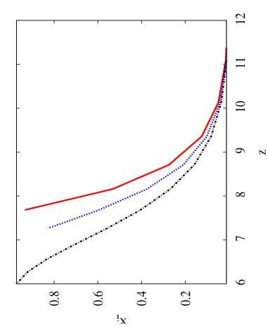
Figure 9: The volume-averaged ionization fraction for simulations M1 (solid curve), M2 (dotted curve), and M3 (dash-dotted curve). In M3 the minihalos absorb more photons than in M2, and there are no minihalos in M1. All simulations have the same source prescription. The presence of minihalos extends the duration of reionization.

Figure 10 shows slices through the M1, M2, and M3 simulations (top, middle, and bottom panels, respectively) at $\bar{x}_{i,V}=0.55$ (left panels) and at $\bar{x}_{i,V}=0.8$ (right panels). [Note that, due to a limited number of outputs at which to compare, the output for simulation M1 is $\approx 7\%$ less ionized than the outputs for the other runs.] The total number of absorptions inside minihalos increases from simulation M1 to M2 to M3. The major effect from minihalo absorptions is that the largest bubbles (bubbles larger than the photon mean free path) grow more slowly, whereas the growth of the smaller bubbles is uninhibited. This effect is particularly noticeable in simulation M3, in which the average mean free path is $4~{}{\rm Mpc}$. The mean free path becomes larger than this as the smallest halos are evaporated in simulation M2, such that the effect of minihalos on the bubble sizes is less significant. The smaller bubbles are still larger in M2 than in M1. (Since M1 is at a $\approx 7\%$ smaller $\bar{x}_{i}$, if we compared at the same $\bar{x}_{i}$, this trend would be more noticeable.)

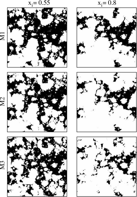
Figure 10: The effect of minihalos on the ionization maps for $\bar{x}_{i,V}\approx 0.55$ (left panels) and $\bar{x}_{i,V}\approx 0.8$ (right panels). The top panels are slices from the M1 simulation in which minihalos do not affect the propagation of the ionization fronts (because we have a limited number of outputs, the top panels are at approximately a $7\%$ lower ionization fraction than the others). White regions are ionized and black are neutral. The middle panels are from M2, in which minihalos are evaporated with a prescription motivated by the results of Shapiro et al. (2004) and Iliev et al. (2005b). The bottom panels are from simulation M3 in which minihalos are not evaporated, and all halos above $10^{5}~{}M_{\odot}$ absorb ionizing photons with impact parameter less than one virial radius (yielding an average photon mean free path of $4~{}{\rm Mpc}$). Minihalos inhibit the largest bubbles from growing.

Figure 11 shows the bubble PDF for the minihalo runs, in which the bubble radius is defined as in §4. We confirm that the bubbles are smaller when the minihalos are present, particularly once the biggest bubbles become larger than the photon mean free path. At $\bar{x}_{i,V}=0.8$, the characteristic bubble radius is $20~{}{\rm Mpc}$ in M1 (solid curve in Fig. 11), $7~{}{\rm Mpc}$ in M2 (dotted curve) , and $4~{}{\rm Mpc}$ in M3 (dot-dashed curve). In the minihalo models, the characteristic scale is set roughly by the average photon mean free path, which is $4~{}{\rm Mpc}$ in simulation M1. This decrease of the characteristic bubble scale from the dense absorbers was first predicted in analytic models (Furlanetto & Oh 2005). However, we do not find the sharp cutoff in effective bubble size at the scale of the mean free path found in the analytic work of Furlanetto & Oh (2005). The reasons for this difference are primarily that analytic models make the simplifying assumptions that the mean free path is spatially uniform and that photons from a source cannot travel a distance further than one mean free path.

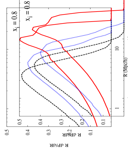
Figure 11: The bubble size distribution for the M1 (solid curve), M2 (dotted curve), and M3 (dot-dashed curve) simulations for $\bar{x}_{i}\approx 0.8$. For the minihalo models, the bubble size peaks at roughly the photon mean free path.

Figure 12 plots $\Delta_{xx}^{2}$ for the M1 (solid curves), M2 (dotted curves), and M3 (dot-dashed curves) simulations for $\bar{x}_{i,V}\approx 0.55$ (top panel) and $\bar{x}_{i,V}\approx 0.8$ (bottom panel). The minihalos suppress the large-scale ionization fluctuations and increase the size of the fluctuations at smaller scales. The significance of the effect of minihalo absorptions increases with ionization fraction as the bubbles become larger. Notice that the total power is contained within the box for the models with minihalos in Figure 12 (the power peaks at smaller scales than the box scale) – the presence of minihalos reduce the size of the box necessary to simulate reionization. Note that the differences in $\Delta_{xx}^{2}$ among the minihalo models we consider (simulations M1–3) are not as large as the differences in $\Delta_{xx}^{2}$ among the source models for $\bar{x}_{i}=0.55$ (simulations S1–S4, Fig. 5). However, for larger ionization fractions (see bottom panel) the effect of minihalos on the structure of reionization can be comparable to the effect of different source models.

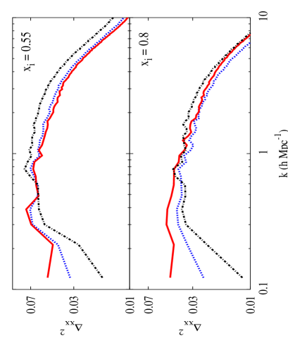
Figure 12: The ionization fraction power spectrum $\Delta_{xx}^{2}$ for the M1 (solid curves), M2 (dotted curves), and M3 (dot-dashed curves) simulations for $\bar{x}_{i}\approx 0.55$ (top panel) and $\bar{x}_{i}\approx 0.8$ (bottom panel). (Note that the snapshot from M1 is really at a $7\%$ lower ionization fraction than the snapshots from M2 and M3 in both panels.) At fixed $\bar{x}_{i}$, the minihalos suppress the large-scale ionization fluctuations and increase the size of the fluctuations at smaller scales.

Dense systems other than minihalos may limit the mean free path of ionizing photons during reionization. Gnedin (2000a) finds that such systems play an important role in reionization in radiative-hydrodynamics simulations. The effect of these “Lyman-limit” systems should be similar to the effect we find for the minihalos.

7 Redshift Dependence

Up to this point, we have only considered reionization scenarios in which overlap occurs at $z\approx 7$ and result in $\tau=0.06-0.08$. However, WMAP’s measurement of $\tau=0.09\pm 0.03$ does not rule out overlap at higher redshifts. Further, the popular conclusion that quasar absorption spectra require that reionization is ending at $z\approx 6.5$ is being hotly debated (Fan et al. 2006; Mesinger & Haiman 2004; Wyithe & Loeb 2004; Lidz et al. 2006a; Becker et al. 2006; Lidz et al. 2006b). At higher redshifts, there are fewer galaxies above $m_{\rm cool}$, enhancing Poisson fluctuations, and the galaxies that do exist are more biased on average. In addition, at higher redshifts the Universe is more dense, resulting in a higher level of recombinations. Finally, at higher redshifts the number of galaxies is growing more quickly, possibly leading to a shorter duration for the reionization epoch. Owing to all these differences, it is interesting to investigate how the structure of reionization when comparing at fixed $\bar{x}_{i}$ changes with redshift. Analytic models predict that the bubble size distribution at fixed $\bar{x}_{i}$ is relatively unchanged with redshift (Furlanetto et al. 2004b)

Figure 13 compares snapshots from the S1 simulation and Z1 simulation, which has the same sources as S1, but where each source has five times the ionizing efficiency. The higher efficiency results in reionization occurring earlier by a redshift interval of $\Delta z\approx 3$. The top panels compare S1 at $z=8.2$ (left) with Z1 at $z=11.1$ (right), both with $\bar{x}_{i,V}\approx 0.3$. The bottom panels compare S1 at $z=7.3$ (left) with Z1 at $z=10.1$ (right), both with $\bar{x}_{i,V}\approx 0.6$. The ionization field is very similar between S1 and Z1 for fixed $\bar{x}_{i}$.

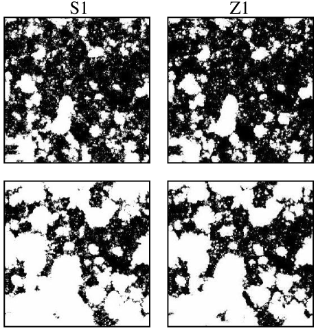
Figure 13: The dependence of the morphology on the redshift of reionization. Slices through snapshots from the S1 and Z1 simulations. Simulation Z1 has the same source prescription as S1, but with five times the ionizing efficiency. The top panels compare S1 at $z=8.2$ (left) and Z1 at $z=11.1$ (right), both with $\bar{x}_{i,V}\approx 0.3$, and the bottom panels compare S1 at $z=7.3$ (left) and Z1 at $z=10.1$ (right), both with $\bar{x}_{i,V}\approx 0.6$. The ionization fields from S1 and Z1 are strikingly similar.

We also ran simulation Z3, which uses the same source prescription as S3 ($\alpha\propto m^{2/3}$), except that the sources in Z3 are five times as efficient as in S3. More massive sources dominate the ionizing efficiency in the S3 and Z3 models than in S1 and Z1. Since the more massive sources are closer to the exponential tail of the Press-Schechter mass function, the part of the mass function which is rapidly changing, we might expect a more significant difference in the ionization maps as we change the redshift of overlap than we found in the previous case. Figure 14 compares the ionization maps for the S3 and Z3 simulations (left and right panels, respectively). The ionization maps are, as with S1 and Z1, very similar. The differences between the $\Delta_{xx}^{2}$ calculated from S1 and Z1 (or from S3 and Z3) are $\lesssim 10\%$ at fixed $\bar{x}_{i}$.

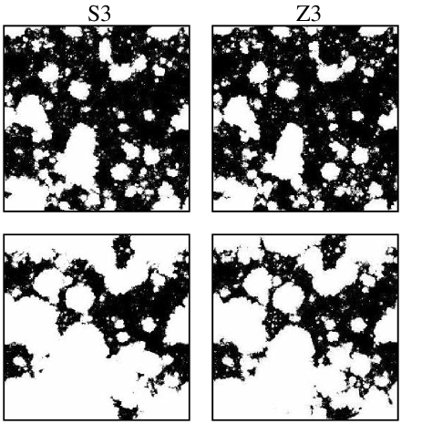
Figure 14: Slices through snapshots from the S3 and Z3 simulations. Simulation Z3 has the same source prescription as S3, but with five times the ionizing efficiency. The top panels compare S3 at $z=8.2$ (left) and Z3 at $z=11.1$ (right), both with $\bar{x}_{i,V}\approx 0.3$, and the bottom panels compare S1 at $z=7.3$ (left) and Z1 at $z=10.1$ (right), both with $\bar{x}_{i,V}\approx 0.6$. The ionization field is very similar between S3 and Z3.

We can understand why the maps look so similar at fixed $\bar{x}_{i}$ by again comparing the power spectra of the sources at these redshifts. The top panel in Figure 2 shows the luminosity-weighted power spectrum $\Delta_{hh}^{2}$ of the sources used the S1/Z1 simulations (solid curves) and S3/Z3 simulations (dotted curves) at $z=6.6$ (thick curves) and $11.1$ (thin curves). The differences between $\Delta_{hh}^{2}$ for the S1 (or S3) sources at $z=6.6$ and at $z=11.1$ are much smaller than the differences between the $\Delta_{hh}^{2}$ for the S1, S3 and S4 source models. Therefore, we would expect the differences between the ionization fields at fixed $\bar{x}_{i}$ but separated by $\Delta z\approx 3$ to be smaller than the differences between the fields for the S1, S3, and S4 models, which is what we find.

Because the ionization maps do not depend strongly on the redshift of reionization, we expect that our conclusions in previous sections hold for slightly higher redshift reionization scenarios. The invariance of the ionization fields with redshift also implies that the conclusions in this paper are not sensitive to the value of $\sigma_{8}$. If reionization occurs at very high redshifts, redshifts where the cooling mass sources are extremely rare, then the topology of reionization will shift from the topology seen in S1 to something closer to what is seen in S4 – the bubbles will become larger and more spherical (see discussion in Zahn et al. (2006b)).

8 Observational Implications

In this section, we briefly discuss the potential of observations to distinguish different reionization models. We limit the discussion to Ly$\alpha$ emitter surveys and 21cm emission. In future work, we will discuss the implications for these and other observations in more detail.

8.1 Ly$\alpha$ Emitter Surveys

Narrow band Ly$\alpha$ emitter surveys are currently probing redshifts as high as $z=6.5$, and projects are in the works to search for higher redshifts Ly$\alpha$ emitters (Kashikawa 2006; Santos et al. 2004; Barton et al. 2004; Iye et al. 2006). If there are pockets of neutral gas at these redshifts, the statistics of these emitters can be dramatically altered (Madau & Rees 2000; Haiman 2002; Santos 2004; Furlanetto et al. 2006a; Malhotra & Rhoads 2006). Sources must be in large HII regions for the Ly$\alpha$ photons to be able to redshift far enough out of the line center to escape absorption. Therefore, the structure of the HII regions will modulate the observed properties of the emitters. Because of this modulation, Ly$\alpha$ emitters could be a sensitive probe of the HII bubbles during reionization. From the current datat on these emitters, there is disagreement as to whether there is evidence for reionization at $z=6.5$ (Kashikawa 2006; Malhotra & Rhoads 2006).

The calculations in this section are all at $z=6.5$, the highest redshift at which there are more than a handful of confirmed Ly$\alpha$ emitters. Rather than re-run our simulations to generate maps with different ionization fractions at $z=6.5$, we instead use the property that the structure of HII regions at fixed $\bar{x}_{i}$ is relatively independent of the redshift (as demonstrated in §7). We take the ionization field from the simulation for higher $z$ and use this field in combination with the $z=6.5$ sources. Since the photo-ionization state of the gas within an HII bubble is dependent on the redshift, we remove the residual neutral fraction within each HII region when calculating the optical depth to absorption $\tau_{{\rm Ly}\alpha}$. The residual neutral gas primarily affects the blue side of the line, which we assume is fully absorbed. We also ignore the peculiar velocity field in this analysis. The peculiar velocities are typically much smaller than the relative velocities due to Hubble expansion between the emitter and its HII front, and, therefore, this omission does not affect our results.

Next, we integrate the opacity along a ray perpendicular to the front of the box from each source to calculate $\tau_{{\rm Ly}\alpha}$. Rather than assume an intrinsic Ly$\alpha$ line profile and follow many frequencies, we calculate the optical depth $\tau_{{\rm Ly}\alpha}$ for a photon that starts off in the frame of the emitter at the line center $\nu_{0}$ and set the observed luminosity $L_{\rm obs,Ly\alpha}=a\,L_{\rm int,Ly\alpha}\,\exp[-\tau_{{\rm Ly}\alpha}(\nu_{0})]$, in which $a$ is a constant of proportionality that encodes the amount of absorption at the line center. For reference, an isolated bubble of $1$ proper Mpc that is fully ionized in the interior has $\tau_{{\rm Ly}\alpha}(\nu_{0})=1$. We also assume the escape fraction is independent of halo mass such that $L_{\rm int,Ly\alpha}=b\,\dot{N}_{\rm UV}$. In future work, we will do a more thorough analysis that includes the velocity field, the neutral fraction within the bubbles, as well as several frequencies around $\nu_{0}$. We also ignore here any stochasticity in the Ly$\alpha$ emission from galaxies. Santos (2004) discusses the importance of many of the effects that are ignored in the calculations in this section.

Figure 15 plots the number density of Ly$\alpha$ emitters with luminosity above $aL_{\rm int,Ly\alpha}$ for several volume-averaged ionization fractions denoted by $x_{i}$ in the plot. We use the fact that there is monotonic relationship between luminosity and mass in our models, which allows us to plot mass on the abscissa. The top panel is from S1 in which $L_{\rm int,Ly\alpha}\propto m$ and the bottom is from S3 in which $L_{\rm int,Ly\alpha}\propto m^{5/3}$. Because the ionizing sources in S3 are rarer, the bubbles are larger and the luminosity function is less suppressed. For both simulations, once the Universe is more than half ionized, the luminosity function is not significantly suppressed at fixed $\bar{x}_{i}$. The normalization of the luminosity function is very sensitive to ionization fractions $\bar{x}_{i}\lesssim 0.5$ in both models.

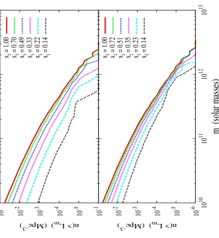
Figure 15: The number density of Ly$\alpha$ emitters above a certain Ly$\alpha$ luminosity $L_{m}=aL_{\rm int,Ly\alpha}$ at $z=6.5$ and for several different volume averaged ionization fractions (denoted by $x_{i}$ in the plot). Here we use the fact that there is monotonic relationship between luminosity and mass in our source models, which allows us to plot halo mass on the abscissa. The top panel is from the S1 simulation in which $L_{\rm int,Ly\alpha}\propto m$ and the bottom is from S3 in which $L_{\rm int,Ly\alpha}\propto m^{5/3}$. Because the sources in S3 are rarer, the bubbles are larger and, therefore, the luminosity function is less suppressed. Current surveys at $z=6.5$ probe a volume of $10^{6}~{}{\rm Mpc}^{3}$ and have found $\approx 100$ emitters.

The luminosity function for different ionized fractions in our calculations is suppressed from the intrinsic luminosity function by a factor that is fairly independent of halo mass (Fig. 15). This prediction for the observed luminosity function is similar to the analytic predictions of Furlanetto et al. (2006a), which use a similar source prescription to that of S1. However, the luminosity function we predict is less suppressed by a factor of $1.5-2$. This small difference is partly because Furlanetto et al. (2006a) underestimates the free path a photon will take inside a bubble. In Furlanetto et al. (2006a), for computational convenience the distance for a photon to travel within a bubble is defined as the distance from the source to the nearest neutral clump rather than the distance along the ray to the bubble edge.

Kashikawa (2006) finds significant evolution in the luminosity function between $z=5.7$ and $z=6.5$ and suggests that this might be evidence for reionization. However, the $z=6.5$ luminosity function differs most with the $z=5.7$ at the high mass end, as opposed to our prediction of it being uniformly suppressed. We suggest that the observed evolution is more consistent with cosmological evolution in the abundance of massive host halos, rather than reflecting an evolving ionized fraction.

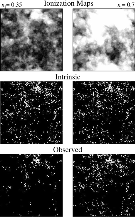
Figure 16: Mock $z=6.5$ Ly$\alpha$ emitter surveys at two different stages of reionization. The left panels are for $\bar{x}_{i,V}=0.35$ and the right are for $\bar{x}_{i,V}=0.7$. The panels would subtend $0.6$ degrees on the sky. All panels use the S1 simulation. Top Panels: A map of the average ionization fraction from a slice through the box of width $31~{}{\rm Mpc}$. In white regions the projection is fully ionized and in black it is fully neutral. Middle Panels: The intrinsic population of Ly$\alpha$ emitters in the same $31~{}{\rm Mpc}$ slice. Our mock survey is sensitive to emitters with halo masses $m>5\times 10^{10}~{}M_{\odot}$. There are $1800$ such halos in the survey, resulting in a density that is an order of magnitude higher than the density probed by current Ly$\alpha$ surveys. Bottom Panels: The observed distribution of Ly$\alpha$ emitters if the Universe is ionized as given in the corresponding top panels. The observed distribution of these emitters is modulated by the presence of HII regions (see top panels for location of HII regions and contrast with intrinsic distribution).

Figure 16 shows maps of the Ly$\alpha$ emitters in simulation S2 with $m>5\times 10^{10}~{}M_{\odot}$. This mock survey would subtend $0.6$ degrees on the sky and has a volume of $3\times 10^{5}~{}{\rm Mpc}^{3}$. The left panels are for $\bar{x}_{i,V}=0.35$ and the right are for $\bar{x}_{i,V}=0.7$. The top panels show the average ionization fraction for a projection of width $31~{}{\rm Mpc}$, corresponding to a narrow band filter with width $\Delta\lambda=100$ angstroms. White regions are fully ionized and black are fully neutral. The middle panels show the intrinsic population of Ly$\alpha$ emitters. There are $1800$ of these halos in the survey; the density of these halos is an order of magnitude higher than the density currently probed by narrow band Ly$\alpha$ surveys. The bottom panels show the observed emitters [with observed luminosity greater than $L_{{\rm int},Ly\alpha}(m=5\times 10^{10}~{}M_{\odot})$], which is modulated by the ionization field in the top panel. In the left, bottom panel, there are 500 visible emitters and in the right, bottom there are 1400. Detecting these large-scale variations in the abundance of Ly$\alpha$ emitters would be a unique signature of patchy reionization. In future work, we calculate several clustering statistics from our emitter maps.

Current surveys at $z=6.5$ are dominated by Poisson fluctuations and are not yet sensitive to density fluctuations or bubble-induced fluctuations from reionization. Figure 16 illustrates, however, that once surveys resolve enough sources then they will be able to detect fluctuations from the HII regions (these fluctuations are generally much larger than the density-induced fluctuations). At larger scales, the bubble fluctuations start to dominate over the Poissonian fluctuations. The fluctuations generated by the bubbles are order unity at the bubble scale, whereas the intrinsic Poisson fluctuations are given by $\Delta(k)^{2}=k^{3}/(2\pi^{2}\,\bar{n})$. If we equate this with unity at $k=0.5\,h\;{\rm Mpc}^{-1}$ (corresponding to a bubble scale of $R=18\,{\rm Mpc}$), we find that surveys must be sensitive to source densities of $\bar{n}=2\times 10^{-3}\;{\rm Mpc}^{-3}$ in order to overcome Poisson noise and be able to image the bubble-induced fluctuations. The requirements for a statistical detection are less stringent. Currently, surveys can probe to densities of $\bar{n}\approx 2\times 10^{-4}\;{\rm Mpc}^{-3}$. In future work, we provide a more quantitative estimate for the number density that surveys must probe to detect reionization.

In future work we will also include the effect of minihalos and gas clumpiness on the Ly$\alpha$ emitters. Minihalos/Lyman-limit systems limit the bubble size and so could potentially suppress the observed luminosity function more substantially than we find in the S1 and S3 simulations.

8.2 21cm Emission

The LOFAR and MWA radio interferometers are being built to observe high redshift neutral hydrogen via the 21cm line, and the GMRT interferometer can already observe at these wavelengths. These telescopes hope to observe an increase in brightness temperature over that of the CMB at wavelengths $\lambda=21{\rm cm}\,(1+z)$ for $z>z_{\rm rei}$ with amplitude

$$T_{21}({\hat{\boldsymbol{n}}},z) = 26\,\left(1-x_{i}({\hat{\boldsymbol{n}}},z)\right)\,\left(1+\delta_{b}({\hat{\boldsymbol{n}}},z)\right)$$ (6)

$$\times \left(\frac{T_{s}({\hat{\boldsymbol{n}}},z)-T_{\rm CMB}(z)}{T_{s}({\hat{\boldsymbol{n}}},z)}\right)\,\left(\frac{\Omega_{B}\,h^{2}}{0.022}\right)$$

$$\times \left(\frac{0.15}{\Omega_{m}\,h^{2}}\,\frac{1+z}{10}\right)^{1/2}~{}{\rm mK},$$

where $T_{s}$ is the spin temperature and $\delta_{b}$ is the baryonic overdensity. Equation (6) (as well as our calculations) neglects redshift-space distortions, which can enhance the signal (Barkana & Loeb 2005). However, these distortions offer only a small enhancement of the signal on the large scales of interest at which ionization fluctuations dominate the signal (McQuinn et al. 2006). We also assume $T_{s}\gg T_{\rm CMB}$ in this section, likely a good approximation during the bulk of the reionization epoch (Ciardi & Madau 2003; Furlanetto 2006).

Figure 17 plots the 21cm power spectrum for the S1 (solid lines), S2 (dashed lines), S3 (dot-dashed lines), and S4 (dotted lines) simulations for $\bar{x}_{i,V}=0.2$ (top panel), $\bar{x}_{i,V}=0.5$ (middle panel), and $\bar{x}_{i,V}=0.7$ (bottom panel). The S3 and S4 simulations have much more power at large scales than the other runs, particularly at early times owing to the larger bubbles in these runs (Fig. 4). The signal is very flat on the scales probed by the box for most $\bar{x}_{i}$. If we had a larger box, a sharp decline in power would be observed at larger scales than the bubbles.

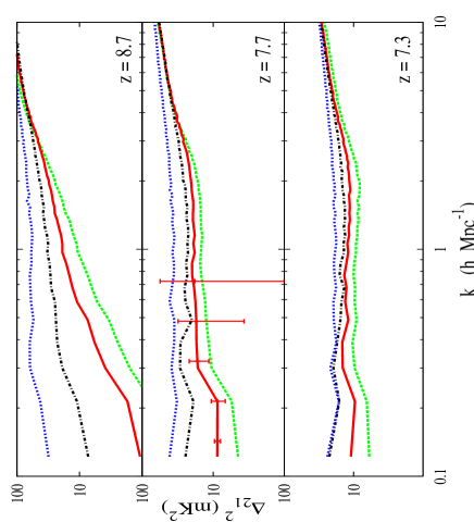
Figure 17: The 21cm power spectrum for the S1 (solid curves), S2 (dashed curves), S3 (dot-dashed curves), and S4 (dotted curves) simulations [$\Delta_{21}^{2}(k)=k^{3}\langle T_{21}(k)^{2}\rangle/2\pi^{2}$]. For the top panels, $\bar{x}_{i,V}\approx 0.2$ ($\bar{x}_{i,M}\approx 0.3$), for the middle panels, $\bar{x}_{i,V}\approx 0.5$ ($x_{i,M}\approx 0.6$), and for the bottom panels, $\bar{x}_{i,V}\approx 0.7$ ($\bar{x}_{i,M}\approx 0.8$). In S2 the lowest mass sources dominate (with masses $m\sim m_{\rm cool}$), and in S4 the highest mass sources dominate ($m\sim 5\times 10^{10}~{}M_{\odot}$). At scales $k\lesssim 1\,h~{}{\rm Mpc}^{-1}$, $\Delta_{21}^{2}$ scales approximately as $\Delta_{xx}^{2}$, such that the 21cm signal is a sensitive probe of the bubble structure. The error bars are the detector noise plus cosmic variance errors on the power spectrum for MWA, assuming $1000$ hours of integration and a bandwidth of $6~{}{\rm MHz}$. Foregrounds will eliminate the sensitivity to the signal for $k\lesssim 0.1~{}h\;{\rm Mpc}^{-1}$.

The power spectra in Figure 17 do not include absorptions from minihalos. If minihalos are as abundant in reality as they are in models M2 and M3, this will suppress significantly the large-scale power in the 21cm signal (see the $\Delta_{xx}$ in Fig. 12). The effect of the minihalos on the 21cm power spectrum is qualitatively different from the effect of changing the sources and should also be observable.

The projected 1-$\sigma$ errors for MWA for a $1000$ hour observation in a 6 MHz band in bins of width $\Delta k=0.5\,k$ are shown in the middle panel in Figure 17. The sensitivity of LOFAR is comparable to that of MWA. The details of this sensitivity calculation are discussed in McQuinn et al. (2006). Because of foregrounds, experiments will encounter difficultly detecting smaller $k$-modes than are plotted here (McQuinn et al. 2006). The first generation of interferometers are most sensitive to $k$ greater than $0.1\,h\;{\rm Mpc}^{-1}$ and less than $1\,h\;{\rm Mpc}^{-1}$. MWA and LOFAR should be able to distinguish between the S1, S3 and S4 reionization scenarios at a fixed ionized fraction. If we marginalize over the ionized fraction, it is unclear whether MWA can still distinguish between these models. The second generation 21cm experiments MWA5000 and SKA will be at least $10\times$ more sensitive than MWA and LOFAR (McQuinn et al. 2006).

In addition, it might be possible to use the evolution of the 21cm signal to separate models. For the models considered in this paper, the duration of reionization is fairly short, spanning an interval of $\delta z=2-4$. It is quite possible that upcoming 21cm experiments will be able to observe the entire breadth of this epoch. The duration of reionization is shortest if the largest mass sources dominate the ionizing budget. Also, minihalos tend to cause a delay at the end of reionization ( Fig. 9). Perhaps combining information on the duration of reionization with the power spectrum at different times can help us understand the source properties as well as the role of the minihalos. Higher order terms in the 21cm power spectrum may aid in distinguishing different reionization scenarios (Lidz et al. 2006c). Zahn et al. (2006a) (in preparation) investigates how well upcoming 21cm experiments can constrain certain reionization models.

9 Conclusions

We have run a suite of $94$ Mpc radiative transfer simulations to understand the size distribution and morphology of HII regions for $0.1<\bar{x}_{i}<0.8$. These simulations are the first that include sources down to the cooling mass and that are large enough to contain many HII regions. We have incorporated structures that all large-scale simulations of reionization do not resolve with analytic prescriptions.

We find that the morphology of HII regions is most sensitive to the parameter $\bar{x}_{i}$. If we compare different reionization scenarios at the same $\bar{x}_{i}$, they tend to look similar. This is not to say other factors besides $\bar{x}_{i}$ do not change the morphology. The sources responsible for reionization are the second most important factor. If we compare at fixed $\bar{x}_{i}$, we find that the HII regions become larger (by as much as a factor of $4$) and more spherical as the sources become rarer. The bubbles are larger for the rarest sources because these sources are the most biased.

The next most important factor for shaping the morphology is the presence of minihalos. Once the mean free path for a photon to intersect a minihalo becomes smaller than the bubble size, the effect of minihalo absorptions becomes important. As a result, minihalos inhibit the largest bubbles from growing. If we use the results of Shapiro et al. (2004) and Iliev et al. (2005b) to characterize the minihalos, we find that these objects have a modest effect on the overall properties of the HII regions at fixed $\bar{x}_{i}$, decreasing $\Delta_{xx}^{2}$ by as much as $50\%$ for the largest modes in our box. In a more extreme case we considered, in which the average mean free path is $4~{}{\rm Mpc}$ during reionization, the impact of minihalos is even more substantial. Minihalos do not have the same effect as changing the source efficiency.

We find that thermal feedback and quasi-linear density inhomogeneities have more minor consequences for the topology of the bubbles at fixed $\bar{x}_{i}$. This is fortunate because these quantities are poorly constrained. Feedback does not substantially change the morphology of reionization at fixed $\bar{x}_{i}$ because the bias difference between the $m>10^{8}~{}M_{\odot}$ halos and the $m>10^{9}~{}M_{\odot}$ halos is relatively small. (The typical halo that is suppressed by feedback is located in a similar region as the typical halo which is not.) Megaparsec-scale, quasi-linear density fluctuations add structure to the boundaries of the HII regions. This additional structure is ignored in analytic models. However, as we increase the level of small-scale gas clumping, either by increasing the resolution or by increasing the subgrid clumping factor, the large-scale structure of the HII regions is largely unaffected at fixed $\bar{x}_{i}$. This is true even if small-scale gas clumping results in a substantial number of recombinations. We find that the $\Delta_{xx}^{2}$ at fixed $\bar{x}_{i}$ differ by no more than $20\%$ as we vary the volume averaged clumping factor from $0$ to $30$. The qualitative reason why clumping does not affect the morphology of reionization at fixed $\bar{x}_{i}$ is because the enhanced photon production in a large-scale overdense region (that is a bubble) is always able to overcome the enhanced number of recombinations, even in extreme clumping models.

The conclusions in this paper hold if overlap occurs at slightly higher redshifts then in our typical simulation in which $z_{\rm overlap}\approx 7$. In fact, we found that if we boosted the source efficiencies such that at $z_{\rm overlap}\approx 10$, the ionization map is essentially unaffected. We showed that this can be explained by the relatively small differences in the luminosity-weighted source power spectrum at $z=7$ compared to that at $z=10$ in the models we considered. The conclusion that the structure of reionization does not depend on the redshift is no longer true if we compare with simulations that reionize at much higher redshifts, redshifts at which the sources become extremely rare. In this case, reionization may have a similar morphology to simulation S4, in which the rarest sources dominate.

In this paper, we did not concentrate on predicting the duration of reionization. However, many of the effects we consider impact the duration of reionization, even if they do not impact the morphology. We find that our most extreme minihalo model extends the duration of reionization by $250$ million years ($\Delta z\approx 1.5$). In addition, feedback on POPII-like ionizing sources from photo-heating can in extreme cases extend reionization by $200$ million years.

Analytic models provide a convenient and intuitive framework to understand the structure of reionization (Furlanetto et al. 2004b, 2005; Zahn et al. 2006b). These models do not suffer from the same scale limitations as simulations, and they supply a quick method to explore the large parameter space relevant to reionization. In addition, these models enhance our physical intuition regarding the processes that shape this epoch. We have confirmed the analytic predictions that the bubble size distribution is approximately log-normal and that the sizes of the bubbles increase as the sources become more biased. Further, we confirm the prediction of analytic models that bubble sizes are largely unchanged if we compare the same model at different redshifts, yet fixed ionized fraction. We also showed, however, that current analytic models encounter some difficulties in describing the effect of minihalos and of Poisson fluctuations in the source abundance on the structure of reionization. Analytic models cannot incorporate the sophisticated models for thermal feedback, gas clumping, and minihalo evaporation that it is possible to include in radiative transfer simulations.

Upcoming observations have potential to distinguish the source models we considered. We make predictions for the luminosity function of Ly$\alpha$ emitters as a function of $\bar{x}_{i}$. We construct maps of Ly$\alpha$ emitters from a mock survey that show large-scale fluctuations in the distribution of emitters due to the HII regions, suggesting that future measurements of the clustering of emitters may reveal the signature of patchy reionization. Future 21cm arrays hold much promise for probing reionization; measurements of the power spectrum with the MWA and the LOFAR arrays can distinguish the S1, S3 and S4 source models.

Upcoming observations can reduce the parameter space that reionization simulations need to explore. If we can measure the number of ionizing photons produced by high mass galaxies and bright quasars at high redshifts, this will reduce the almost total freedom we currently have in the ionizing luminosity. Observations of the mean free path of ionizing photons at high redshifts may reveal whether the Lyman-limit systems are the minihalos as well as how fast these systems are being evaporated. A precise measurement of the Thomson scattering optical depth from the CMB will constrain the average redshift of reionization.

It is important to continue to improve large-scale simulations of reionization to understand the reionization process in more detail. Future simulations need to investigate the effect of more realistic star formation models, metal pollution, and alternative sources of ionizing photons. In addition, larger simulations than are presented here are necessary to statistically describe this epoch for $\bar{x}_{i}\gtrsim 0.7$. It is also useful to run small-scale simulations to develop more realistic subgrid parameterizations for the minihalos and for the clumping factor. These parameterizations will be essential for modeling the end of reionization, a time when the rate of evaporation of the Lyman-limit systems plays a key role in determining the structure of reionization. Also, such parameterizations are necessary to extend our calculations to model accurately the part in $10^{4}$ neutral fraction fluctuations that characterize the high redshift Ly$\alpha$ forest.

An accurate interpretation of future observations of reionization, while certainly challenging, does not appear impossible. The characteristics of HII regions during reionization might have depended on a huge number of poorly constrained parameters, making it impossible to interpret observations of this epoch. We find that this is not the case. The morphology of the HII regions at fixed $\bar{x}_{i}$ boils down primarily to the properties of the sources and of the minihalos/Lyman-limit systems.

10 acknowledgments

We thank Mark Dijkstra for helpful conversations regarding thermal feedback and Ly$\alpha$ emitters, Volker Springel for providing his Lean Gadget–2 code, Roman Scoccimarro for providing his 2LPT code, and Steven Furlanetto for useful comments on the manuscript. MM would like to thank the NSF graduate student fellowship. The authors are also supported by the David and Lucile Packard Foundation, the Alfred P. Sloan Foundation, and NASA grants AST-0506556 and NNG05GJ40G.

Appendix A Radiative Transfer Algorithm

For the simulations in this paper, we employ the Sokasian et al. (2001, 2003, 2004) cosmological radiative transfer code, but with several significant changes that are discussed below. This algorithm inputs grids of the density field as well as a list of sources and then casts rays from every source, randomizing the order of the sources within this loop. Radiative feedback on the density field is ignored. Rays are split adaptively using the HealPIX algorithm (Abel & Wandelt 2002) such that, at a minimum, $N$ rays from a source intersect every cell face (for this paper, we set $N=2.1$). This algorithm does not iterate the ray casting within each time step to converge to the correct ionized fraction in each cell. Instead, once a cell has been ionized by a source within a time step, rays from other sources will pass through it. This simplification allows for the algorithm to process more sources and larger volumes than other codes. In the limit of few sources and few time steps, this simplification can lead to artificial structure in the HII regions. However, with the vast number of sources in the simulations in this paper, even with relatively coarse time steps we choose, this artificial structure is minimized (as we will demonstrate later in this section).

The temperature history of the gas is not tracked by this code. Instead, the code assumes that ionized regions are at $T=10^{4}$ Kelvin. The temperature affects the number of recombinations in the simulation because $\alpha_{B}\propto T^{-0.7}$, as well as the detailed photo-ionization state of the gas within the HII regions. The analysis we have done in this paper does not depend on the photo-ionization state of the gas. In addition, the value for the subgrid clumping factor, which determines the number of recombinations with in a cell, is highly uncertain, such that we would not gain any precision from including a full calculation of the IGM temperature.

What follows is a list of the important modifications that we have made to the original Sokasian et al. (2001) algorithm:

• Previously, cells were either ionized or neutral. Cells can now be fractionally ionized. We assume that the ionizing front is paper thin such that each cell can be broken up into a neutral part and an ionized part.

• Each ray holds a number of photons. In the original Sokasian et al. (2001) algorithm, the first ray that hit a cell from a particular source carried all the information that the cell needed about the source. Subsequent rays from the same source did not affect the cell. The advantage to having each ray contain a specific number of photons is that it is trivial to conserve photons as well as to include photon sinks. The disadvantage is that the ionization front has a numerical width that is wider than in the previous algorithm. We find that the width of the front in the new algorithm is approximately $2$ cells for a single source. The thickness of the front is smaller than $2$ cells in the limit relevant to this paper of many faint sources.

• The orientation of the HealPIX ray casting scheme is randomly rotated between each time step, and the order with which the rays are initially cast is also randomized. When rays split adaptively, the order is again randomized over the daughter rays. All of this randomization is done to minimize artifacts owing to the order in which operations are performed.

• Once a ray has traveled a distance equal to $\eta\,R_{\rm box,proper}\,[3\dot{N}_{source}/(4\pi\dot{N}_{\rm box})]^{1/3}$, it can no longer split into daughter rays, where $\dot{N}_{\rm source}$ is the ionizing luminosity from the source and $\dot{N}_{\rm box}$ is the total luminosity of all the sources in the box. We set $\eta=5$ for this paper. Until this distance, rays split adaptively such that a set number of rays intersect every cell face. This simplification is justified by the large numbers of sources in an HII region (typically more than $1000$ sources), making it unnecessary to have rays from one side of an HII region cover the entire front on the other side. Our approximation results in the correct fluxes in the cells in the limit of many sources. We have investigated quantitatively whether this simplification makes a difference in the ionization maps. The middle panel in Figure 19 plots the cross correlation coefficient at two times between a simulation with no ray termination and a simulation with the prescription for ray termination used in this paper (see the caption in Fig. 19 for the definition of the cross correlation coefficient). There is essentially no difference between the maps. This simplification results in the algorithm running over a factor of $5$ faster at high ionized fractions.

• The previous algorithm reset the density in each cell after a time step to the density field in the next snapshot, but did not change the ionized fraction in the cell to account for the dynamics of the ionization field. For example, a cell that becomes fully ionized would remain fully ionized in subsequent time steps (neglecting recombinations), even if it gained neutral material from a neighboring cell during these time steps. This resulted in the total number of ionized atoms not being conserved by the previous algorithm between time steps. To remedy this issue in the current algorithm, we account for a dynamic density field by assigning some ionization fraction to each particle in the N-body simulation and then re-gridding the ionization map between time steps to account for the particle dynamics. We suspect that other cosmological radiative transfer algorithms performed on top of a static density grid ignore the dynamics of the ionization field in their computations.

• N-body particles that are associated with halos are not included in the density field used by the radiative transfer algorithm. Otherwise, cells with sources would have substantial overdensities, and ionizing photons from within the cell would have to ionize these cells prior to escaping into the IGM. These absorptions are already counted in the escape fraction. Removing the halo particles from the gridded density field is also appropriate for rays incident on this cell. The gas in the massive source halos has cooled to form a small disk that is much smaller than the cross section of the cell. Therefore, the vast majority of photons coming from exterior to the cell do not intersect this disk. The gas within galaxies during reionization absorbs a negligible amount of external photons because the mean free path of these photons to intersect a galaxy is large (larger than the $94$ Mpc box size employed in this paper).

We subjected the radiative transfer algorithm to several tests. As a simple test, we put one source with $\dot{N}=10^{56}\,{\rm photons~{}}{\rm s}^{-1}$ in a $65.6$ Mpc/h box with $256^{3}$ cells, with each cell at the mean density of the $z=6$ Universe, and set the clumping factor $C$ in each cell to $C=1$ or $C=30$. In Figure 18, we compare the fraction of the box that is ionized in this test to the fraction that is predicted by theory (using coarse time steps of $5\times 10^{7}$ years). Even with such coarse time steps, this algorithm matches the theory curves well.

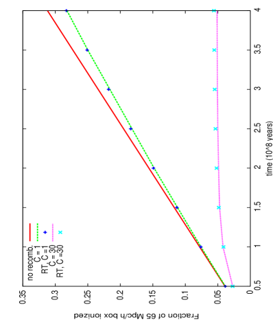
Figure 18: The fraction of the simulation box that is ionized by a single source with $\dot{N}=10^{56}~{}s^{-1}$. This calculation is performed at $z=6$ with all cells at the mean density of the Universe and with the subgrid clumping factor $C$ equal to $1$ and $30$. The solid, dashed and dotted curves are from a theoretical calculation for no recombinations, recombinations with $C=1$ and recombinations with $C=30$, respectively. The pluses and crosses are the radiative transfer algorithm with $C=1$ and $C=30$ with coarse time steps of $\Delta t=5\times 10^{7}$ years. The radiative transfer agrees well with the theoretical result, slightly under-predicting the number of recombinations.

Because the algorithm does not iterate to find the ionized fraction, this might lead to artificial structure if the time step is too coarse. In the limit of an infinitely small time step, this algorithm gives us the exact solution. In this paper we use a time step of $50$ million years. To test convergence, we run two cosmological simulations on the $256^{3}$ grid (which we label simulation 1 and 2), using the halos with $m>2\times 10^{9}~{}M_{\odot}$ as our sources. Each simulation uses a different set of random numbers to establish the order of the sources for ray casting. If the 50 million year time step is too coarse, the ionization maps from these two simulations would differ substantially, whereas the time step is sufficiently small if the ionization maps differ insignificantly. The bottom panel of Figure 19 plots the cross correlation coefficient $r=P_{x_{1}x_{2}}/\sqrt{P_{x_{1}x_{1}}\,P_{x_{2}x_{2}}}$ between these two runs for ionization fractions of $\bar{x}_{i}=0.2$ (solid curves) and $\bar{x}_{i}=0.7$ (dashed curves). The cross correlation coefficient is close to unity at most scales, dropping to $0.8$ at the cell scale. Note that the cross correlation coefficient is a stringent test. We have also looked at the power spectrum of these runs. The power spectrum of the ionized fraction differs negligibly between these two runs, differing by about $0.3\%$ at $k=10~{}h~{}{\rm Mpc}^{-1}$ and $1.5\%$ at $k=20~{}h~{}{\rm Mpc}^{-1}$.

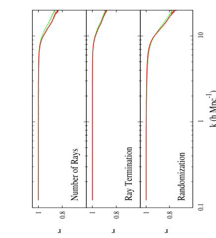
Figure 19: The cross correlation coefficient $r=P_{x_{1}x_{2}}(k)/\sqrt{P_{x_{1}x_{1}}(k)\,P_{x_{2}x_{2}}(k)}$ between the ionization maps from different simulations. All panels are run with $\dot{N}(m)=3\times 10^{49}\;m/(10^{8}~{}M_{\odot})~{}s^{-1}$ and using only halos with $m>2\times 10^{9}~{}M_{\odot}$. The cell scale is at $k\approx 20~{}h\;{\rm Mpc}^{-1}$. Top Panels: The cross correlation coefficient for a simulation that casts $64$ times the number of initial rays and ensures that $2$ times more rays intersect every cell as in the fiducial runs. The solid curve is for $\bar{x}_{i}=0.2$ and the dashed is for $\bar{x}_{i}=0.5$. Middle Panels: The cross correlation coefficient of a simulation that terminates rays with the condition given in this section versus a simulation with no ray termination. The solid curve is for $\bar{x}_{i}=0.3$ and the dashed is for $\bar{x}_{i}=0.5$. The maps are extremely similar even though the simulation without ray casting took five times longer to reach $\bar{x}_{i}=0.5$. Bottom Panels: Cross correlation coefficient for two runs with two different sets of random numbers. The random numbers set the order of the sources for ray casting. The solid curve is for $\bar{x}_{i}=0.2$ and the dashed is for $\bar{x}_{i}=0.7$. All panels show that the ionization field has converged sufficiently in our simulations.

We have also investigated whether the ionization structure seen in our fiducial runs has converged to the true structure by either increasing the number of rays that are cast or by increasing the mesh size to $512^{3}$. First, we ran with a simulation that casts a much larger number of rays per source than the fiducial number of rays ($64\times$ more initially and with the criteria that a minimum of $4.1$ rather than $2.1$ rays intersect every cell). We find that the fiducial number of rays is enough to capture the structure of the HII region (top panel, Fig. 19). Second, we have run a resolution test, comparing a higher resolution $512^{3}$ radiative transfer simulation without recombinations to a $256^{3}$ run without recombinations. We re-grid the $512^{3}$ snapshots to $256^{3}$ resolution for comparison. We find that for all $\bar{x}_{i}$ the power spectra have converged to within $10\%$ at scales with $k<10~{}h\;{\rm Mpc}^{-1}$. The agreement is even better then this for $\bar{x}_{i}>0.5$.

The computation speed of this code scales in a time step as $N_{r}\,R^{2}\,N_{s}$ where $N_{r}$ is the number of rays through each cell, $R$ is the characteristic bubble size, $N_{s}$ is the number of sources. When the bubbles are large, the code slows down considerably. We are working on ways to ameliorate this issue with the code. Most simulations in this paper took less than two days to reach $\bar{x}_{i}=0.8$ on a single $2.2$ GHz AMD Opteron processor.

Appendix B Fitting Formula for Minihalo Evaporation

Iliev et al. (2005b) provide fitting formula for the evaporation of minihalos by POPII stars. These simulations do full radiative hydrodynamics on minihalos, which are modeled prior to front crossing as truncated isothermal spheres (TIS) with self similar infall. They provide the formula for the evaporation timescale

$$t_{\rm ev} = 150\,\left(\frac{M}{10^{7}~{}M_{\odot}}\right)^{0.434}\,F^{-0.35+0.05\,\log_{10}(F)}$$ (7)

$$\times\left[0.1+0.9\,\left(\frac{1+z}{10}\right)\right]~{}{\rm Myr},$$

where $F$ is the flux (which is time-independent in their simulations). To apply these formula to simulation M2, we use for $F$ the time averaged flux incident on a cell, with averaging starting after the cell becomes ionized.

In Figure 29 in Shapiro et al. (2004), the effective cross section of a halo for absorbing an ionizing photon as a function of time is plotted for a $10^{7}~{}M_{\odot}$ halo. Iliev et al. (2005b) does not provide parameterized fits to the effective cross section, which we need in our calculations. To proceed, we fit by eye the curve for the effective cross section in Shapiro et al. (2004). We find the function

$$\frac{\sigma_{\rm mh}}{\pi\,r_{t}^{2}}=\frac{1}{3}\times 10^{-1.7\,\left(\frac{t}{t_{\rm ev}}\right)^{1.5}},$$ (8)

where $r_{t}=0.754\,[M/(10^{7}\,M_{\odot})]^{1/3}\,10/(1+z)$ is the scale radius for the TIS profile. By construction in the simulations of Shapiro et al. (2004), $\sigma_{\rm mh}=\pi\,r_{t}^{2}$ at $t=0$. However, on a timescale of order a million years the outskirts of the halo are evaporated, consuming a meager amount of photons. The denser inner regions take a significantly longer time to evaporate. We set $\sigma_{\rm mh}=\pi\,r_{t}^{2}$ for the first $5$ million years, and subsequently use equation (8) in run M2. Of course, the function we use for $\sigma_{\rm mh}$ likely does not scale correctly with redshift or halo mass. We anticipate that it over-predicts the cross section for halos with $m<10^{7}~{}M_{\odot}$, since the gas in the outskirts of these smaller halos will be easier to evaporate.

Appendix C Filtering Mass

If all of the gas in the IGM is cold before reionization and subsequently jumps to $10^{4}$ K at $a_{\rm rei}$, the filtering mass is (Gnedin & Hui 1998)

$$M_{f}=M_{\rm J}\,\left(\frac{3}{10}\left[1+4\left(\frac{a_{\rm rei}}{a}\right)^{5/2}-5\left(\frac{a_{\rm rei}}{a}\right)^{2}\right]\right)^{3/2}.$$ (9)

This mass scale can be much smaller than the Jeans mass for $10^{4}$ K gas $M_{\rm J}$ and is typically time dependent. Since $M_{f}$ typically corresponds to non-linear scales where linear theory is a poor approximation, it is unclear how well equation (9) represents the smallest mass at which the baryons clump. However, Gnedin & Hui (1998) smooth N-body simulations by including a pressure force that becomes important at the filtering scale. They conclude that this procedure reproduces well the small-scale gas power spectrum seen in hydrodynamics simulations. Furthermore, Gnedin (2000b) finds that the filtering mass provides a good fit to the minimum formation mass for a gas-rich halo.

References

- Abel & Wandelt (2002) Abel, T., & Wandelt, B. D. 2002, MNRAS, 330, L53
- Barkana & Loeb (1999) Barkana, R., & Loeb, A. 1999, ApJ, 523, 54
- Barkana & Loeb (2002) Barkana, R., & Loeb, A. 2002, ApJ, 578, 1
- Barkana & Loeb (2004) Barkana, R., & Loeb, A. 2004, ApJ, 609, 474
- Barkana & Loeb (2005) Barkana, R., & Loeb, A. 2005, ApJL, 624, L65
- Barton et al. (2004) Barton, E. J., et al. 2004, Astrophys. J., 604, L1
- Becker et al. (2006) Becker, G. D., Rauch, M., & Sargent, W. L. W. 2006, ArXiv Astrophysics e-prints
- Becker et al. (2001) Becker, R. H., et al. 2001, AJ, 122, 2850
- Bond et al. (1991) Bond, J. R., Cole, S., Efstathiou, G., & Kaiser, N. 1991, ApJ, 379, 440
- Ciardi & Madau (2003) Ciardi, B., & Madau, P. 2003, ApJ, 596, 1
- Ciardi et al. (2006) Ciardi, B., Scannapieco, E., Stoehr, F., Ferrara, A., Iliev, I. T., & Shapiro, P. R. 2006, MNRAS, 366, 689
- Ciardi et al. (2003) Ciardi, B., Stoehr, F., & White, S. D. M. 2003, MNRAS, 343, 1101
- Cohn & Chang (2006) Cohn, J. D., & Chang, T. 2006, astro-ph/0603438
- Crocce et al. (2006) Crocce, M., Pueblas, S., & Scoccimarro, R. 2006, astro-ph/0606505
- Dijkstra et al. (2004) Dijkstra, M., Haiman, Z., Rees, M. J., & Weinberg, D. H. 2004, ApJ, 601, 666
- Fan et al. (2006) Fan, X., et al. 2006, AJ, 132, 117
- Furlanetto (2006) Furlanetto, S. 2006, astro-ph/0604040
- Furlanetto et al. (2004a) Furlanetto, S. R., Hernquist, L., & Zaldarriaga, M. 2004a, MNRAS, 354, 695
- Furlanetto et al. (2005) Furlanetto, S. R., McQuinn, M., & Hernquist, L. 2005, MNRAS, 1043
- Furlanetto & Oh (2005) Furlanetto, S. R., & Oh, S. P. 2005, MNRAS, 363, 1031
- Furlanetto et al. (2004b) Furlanetto, S. R., Zaldarriaga, M., & Hernquist, L. 2004b, ApJ, 613, 1
- Furlanetto et al. (2004c) Furlanetto, S. R., Zaldarriaga, M., & Hernquist, L. 2004c, ApJ, 613, 16
- Furlanetto et al. (2006a) Furlanetto, S. R., Zaldarriaga, M., & Hernquist, L. 2006, Mon. Not. Roy. Astron. Soc., 365, 1012
- Furlanetto et al. (2006b) Furlanetto, S. R., Oh, P. S., & Briggs, F. 2006, astro-ph/0608032
- Gnedin (2000a) Gnedin, N. Y. 2000a, ApJ, 535, 530
- Gnedin (2000b) Gnedin, N. Y. 2000b, ApJ, 542, 535
- Gnedin & Hui (1998) Gnedin, N. Y., & Hui, L. 1998, MNRAS, 296, 44
- Haiman (2002) Haiman, Z. 2002, Astrophys. J., 576, L1
- Haiman et al. (2000) Haiman, Z., Abel, T., & Rees, M. J. 2000, ApJ, 534, 11
- Haiman & Loeb (1999) Haiman, Z., & Loeb, A. 1999, ApJ, 519, 479
- Haiman et al. (1997) Haiman, Z., Rees, M. J., & Loeb, A. 1997, ApJ, 476, 458
- Hopkins et al. (2006a) Hopkins, P. F., Hernquist, L., Cox, T. J., Di Matteo, T., Robertson, B., & Springel, V. 2006a, ApJS, 163, 1
- Hopkins et al. (2006b) Hopkins, P. F., Somerville, R. S., Hernquist, L., Cox, T. J., Robertson, B., & Li, Y. 2006b, ApJ, submitted, astro-ph/0602290
- Hui et al. (2002) Hui, L., Haiman, Z., Zaldarriaga, M., & Alexander, T. 2002, ApJ, 564, 525
- Iliev et al. (2006a) Iliev, I. T., Mellema, G., Pen, U.-L., Merz, H., Shapiro, P. R., & Alvarez, M. A. 2006a, MNRAS, 369, 1625
- Iliev et al. (2005a) Iliev, I. T., Scannapieco, E., & Shapiro, P. R. 2005a, ApJ, 624, 491
- Iliev et al. (2005b) Iliev, I. T., Shapiro, P. R., & Raga, A. C. 2005b, MNRAS, 361, 405
- Iliev et al. (2006b) Iliev, I. T., et al. 2006b, astro-ph/0607209
- Iliev et al. (2006c) Iliev, I. T., et al. 2006c, astro-ph/0607517
- Iye et al. (2006) Iye, M., et al. 2006, astro-ph/0609393
- Kashikawa (2006) Kashikawa, N. 2006, astro-ph/0604149
- Kauffmann et al. (2003) Kauffmann, G., et al. 2003, MNRAS, 341, 33
- Kitayama et al. (2001) Kitayama, T., Susa, H., Umemura, M., & Ikeuchi, S. 2001, MNRAS, 326, 1353
- Kitayama et al. (2000) Kitayama, T., Tajiri, Y., Umemura, M., Susa, H., & Ikeuchi, S. 2000, MNRAS, 315, L1
- Kohler et al. (2005) Kohler, K., Gnedin, N. Y., & Hamilton, A. J. S. 2005, astro-ph/0511627
- Kramer et al. (2006) Kramer, R. H., Haiman, Z., & Oh, S. P. 2006, astro-ph/0604218
- Li et al. (2006) Li, Y., et al. 2006, ApJ, submitted [astro-ph/0608190]
- Lidz et al. (2006a) Lidz, A., Oh, S. P., & Furlanetto, S. R. 2006a, ApJL, 639, L47
- Lidz et al. (2006b) Lidz, A., et al. 2006b, in prep
- Lidz et al. (2006c) Lidz, A., et al. 2006c, ApJ, submitted [astro-ph/0610054]
- Madau & Rees (2000) Madau, P., & Rees, M. J. 2000, ApJL, 542, L69
- Malhotra & Rhoads (2006) Malhotra, S., & Rhoads, J. E. 2006, ApJL, 647, L95
- McQuinn (2006) McQuinn, M. 2006, unpublished work (email mmcquinn@cfa.harvard.edu for transcript)
- McQuinn et al. (2005) McQuinn, M., Furlanetto, S. R., Hernquist, L., Zahn, O., & Zaldarriaga, M. 2005, ApJ, 630, 643
- McQuinn et al. (2006) McQuinn, M., Zahn, O., Zaldarriaga, M., Hernquist, L., & Furlanetto, S. R. 2006, astro-ph/0512263
- Mellema et al. (2006) Mellema, G., Iliev, I. T., Pen, U.-L., & Shapiro, P. R. 2006, MNRAS, 1014
- Mesinger & Haiman (2004) Mesinger, A., & Haiman, Z. 2004, ApJL, 611, L69
- Miralda-Escudé et al. (2000) Miralda-Escudé, J., Haehnelt, M., & Rees, M. J. 2000, ApJ, 530, 1
- Mo & White (1996) Mo, H. J., & White, S. D. M. 1996, MNRAS, 282, 347
- Osterbrock (1989) Osterbrock, D. E. 1989, Astrophysics of Gaseous Nebulae and Active Galactic Nuclei (Sausalito, CA: University Science Books)
- Press & Schechter (1974) Press, W. H., & Schechter, P. 1974, ApJ, 187, 425
- Santos (2004) Santos, M. R. 2004, Mon. Not. Roy. Astron. Soc., 349, 1137
- Santos et al. (2004) Santos, M. R., Ellis, R. S., Kneib, J.-P., Richard, J., & Kuijken, K. 2004, ApJ, 606, 683
- Scoccimarro & Sheth (2002) Scoccimarro, R., & Sheth, R. K. 2002, MNRAS, 329, 629
- Shapiro et al. (2004) Shapiro, P. R., Iliev, I. T., & Raga, A. C. 2004, MNRAS, 348, 753
- Sheth & Lemson (1999) Sheth, R. K., & Lemson, G. 1999, MNRAS, 305, 946
- Sheth & Tormen (2002) Sheth, R. K., & Tormen, G. 2002, MNRAS, 329, 61
- Sokasian et al. (2001) Sokasian, A., Abel, T., & Hernquist, L. 2001, NewA, 6, 359
- Sokasian et al. (2003) Sokasian, A., Abel, T., Hernquist, L., & Springel, V. 2003, MNRAS, 344, 607
- Sokasian et al. (2004) Sokasian, A., Yoshida, N., Abel, T., Hernquist, L., & Springel, V. 2004, MNRAS, 350, 47
- Spergel et al. (2003) Spergel, D. N., et al. 2003, ApJS, 148, 175
- Spergel et al. (2006) Spergel, D. N., et al. 2006, astro-ph/0603449
- Springel (2005) Springel, V. 2005, MNRAS, 364, 1105
- Springel & Hernquist (2003) Springel, V., & Hernquist, L. 2003, MNRAS, 339, 312
- Stark et al. (2006) Stark, D. P., Bunker, A. J., Ellis, R. S., Eyles, L. P., & Lacy, M. 2006, astro-ph/0604250
- Totani et al. (2006) Totani, T., Kawai, N., Kosugi, G., Aoki, K., Yamada, T., Iye, M., Ohta, K., & Hattori, T. 2006, PASJ, 58, 485
- Viel et al. (2006) Viel, M., Haehnelt, M. G., & Lewis, A. 2006, Mon. Not. Roy. Astron. Soc. Lett., 370, L51
- White et al. (2003) White, R. L., Becker, R. H., Fan, X., & Strauss, M. A. 2003, AJ, 126, 1
- Wood & Loeb (2000) Wood, K., & Loeb, A. 2000, ApJ, 545, 86
- Wyithe & Loeb (2003) Wyithe, J. S. B., & Loeb, A. 2003, ApJ, 586, 693
- Wyithe & Loeb (2004) Wyithe, J. S. B., & Loeb, A. 2004, Nature, 427, 815
- Zahn et al. (2005) Zahn, O., Zaldarriaga, M., Hernquist, L., & McQuinn, M. 2005, Astrophys. J., 630, 657
- Zahn et al. (2006a) Zahn, O., et al. 2006a, in prep
- Zahn et al. (2006b) Zahn, O., et al. 2006b, astro-ph/0604177
- Zaldarriaga et al. (2004) Zaldarriaga, M., Furlanetto, S. R., & Hernquist, L. 2004, ApJ, 608, 622