Crossing the Phantom Divide: Theoretical Implications and Observational Status

Abstract

If the dark energy equation of state parameter $w(z)$ crosses the phantom divide line $w=-1$ (or equivalently if the expression $\frac{d(H^{2}(z))}{dz}-3\Omega_{0m}H_{0}^{2}(1+z)^{2}$ changes sign) at recent redshifts, then there are two possible cosmological implications: Either the dark energy consists of multiple components with at least one non-canonical phantom component or general relativity needs to be extended to a more general theory on cosmological scales. The former possibility requires the existence of a phantom component which has been shown to suffer from serious theoretical problems and instabilities. Therefore, the latter possibility is the simplest realistic theoretical framework in which such a crossing can be realized. After providing a pedagogical description of various dark energy observational probes, we use a set of such probes (including the Gold SnIa sample, the first year SNLS dataset, the 3-year WMAP CMB shift parameter, the SDSS baryon acoustic oscillations peak (BAO), the X-ray gas mass fraction in clusters and the linear growth rate of perturbations at $z=0.15$ as obtained from the 2dF galaxy redshift survey) to investigate the priors required for cosmological observations to favor crossing of the phantom divide. We find that a low $\Omega_{0{\rm m}}$ prior ($0.2<\Omega_{0{\rm m}}<0.25$) leads, for most observational probes (except of the SNLS data), to an increased probability (mild trend) for phantom divide crossing. An interesting degeneracy of the ISW effect in the CMB perturbation spectrum is also pointed out.

I Introduction

The assumption of large scale homogeneity and isotropy of the universe combined with the assumption that general relativity is the correct theory on cosmological scales leads to the Friedman equation which in a flat universe takes the form

$$H^{2}(a)=\left(\frac{{\dot{a}}}{a}\right)^{2}=\frac{8\pi G}{3}\rho(a)$$ (1)

where $a(t)$ is the scale factor of the universe and $\rho$ its average energy density. Both sides of this equation can be observationally probed directly: The left side using mainly geometrical methods (measuring the luminosity and angular diameter distances $d_{L}(z)$snobs ; Riess:2004nr ; Astier:2005qq and $d_{A}(z)$Eisenstein:2005su ; Allen:2002sr ; Allen:2004cd ; Spergel:2006hy with standard candles and standard rulers) showing an accelerating expansion at recent redshifts and the matter - radiation density part of the right side using dynamical and other methods (cosmic microwave background Spergel:2006hy , large scale structure observationsVerde:2001sf , lensingHoekstra:2002xs etc). These observations have indicatedSahni:1999gb that the two sides of the Friedman equation (1) can not be equal if $\rho(a)=\rho_{m}(a)\sim a^{-3}$ even if a non-zero curvature is assumed. There are two possible resolutions to this puzzle: Either modify the right side of the Friedman equation (1) introducing a new form of ‘dark’ energy ideal fluid component ($\rho(a)=\rho_{m}(a)+\rho_{X}(a)$) with suitable evolution in order to restore the equality or modify both sides by changing the way energy density affects geometry thus modifying the Einstein equations.

In the first class of approaches the required gravitational properties of dark energy (see Copeland:2006wr ; Padmanabhan:2006ag ; Perivolaropoulos:2006ce ; Straumann:2006tv ; Uzan:2006mf ; Sahni:2006pa for recent reviews) needed to induce the accelerating expansion are well described by its equation of state $w(z)=\frac{p_{X}(z)}{\rho_{X}(z)}$ which enters in the second Friedman equation as

$$\frac{{\ddot{a}}}{a}=-\frac{4\pi G}{3}(\rho_{m}+\rho_{X}(1+3w))$$ (2)

implying that a negative pressure ($w<-1/3$) is necessary in order to induce accelerating expansion. The simplest viable example of dark energy is the cosmological constantSahni:1999gb ; Peebles:2002gy ; Carroll:2000fy ($w=-1$). This example however even though consistent with present data lacks physical motivation. Questions like ‘What is the origin of the cosmological constant?’ or ‘Why is the cosmological constant $10^{120}$ times smaller than its natural scale so that it starts dominating at recent cosmological times (coincidence problem)?’ remain unansweredWeinberg:2000yb . Attempts to replace the cosmological constant by a dynamical scalar field (quintessenceCaldwell:1997ii ; Zlatev:1998tr ; Ratra:1987rm ) have created a new problem regarding the initial conditions of quintessence which even though can be resolved in particular cases (tracker quintessence), can not answer the above questions in a satisfactory way.

The parameter $w(z)$ determines not only the gravitational properties of dark energy but also its evolution. This evolution is easily obtained from the energy momentum conservation

$$d(\rho_{X}a^{3})=-p_{X}d(a^{3})$$ (3)

which leads to

$$\rho_{X}=\rho_{0X}e^{-3\int_{1}^{a}\frac{da^{\prime}}{a^{\prime}}(1+w(a^{\prime}))}=\rho_{0X}e^{3\int_{0}^{z}\frac{dz^{\prime}}{1+z^{\prime}}(1+w(z^{\prime}))}$$ (4)

Therefore the determination of $w(z)$ is equivalent to that of $\rho_{X}(z)$ which in turn is equivalent to the observed $H(z)$ from the Friedman equation (1) expressed as

$$H(z)=H_{0}[\Omega_{0{\rm m}}(1+z)^{3}+\Omega_{0X}e^{3\int_{0}^{z}\frac{dz^{\prime}}{1+z^{\prime}}(1+w(z^{\prime}))}]$$ (5)

Thus, knowledge of $\Omega_{0{\rm m}}$ and $H(z)$ suffices to determine $w(z)$ which is obtained from equation (5) as Huterer:2000mj

$$w(z)=\frac{\frac{2}{3}(1+z)\frac{dlnH}{dz}-1}{1-\frac{H_{0}^{2}}{H^{2}}\Omega_{0{\rm m}}(1+z)^{3}}$$ (6)

In the second class of approaches the Einstein equations get modified and the new equations combined with the assumption of homogeneity and isotropy lead to a generalized Friedman equation of the form

$$f(H^{2})=g(\rho_{m})$$ (7)

where $f$ and $g$ are appropriate functions determined by the modified gravity theoryBoisseau:2000pr ; Nojiri:2006je ; Sahni:2002dx ; Chimento:2006ac ; Carroll:2004de ; Deffayet:2000uy . In this class of models, the parameter $w(z)$ can also be defined from equation (6) but it can not be interpreted as $\frac{p_{X}}{\rho_{X}}$ of a perfect fluid.

The simplest (but quite general) examples of modified gravity theories are scalar tensor theoriesBoisseau:2000pr ; Esposito-Farese:2000ij ; Torres:2002pe ; Gannouji:2006jm ; Perivolaropoulos:2005yv where the Newton’s constant $G$ is promoted to a function of a field $\Phi$: $8\pi G\rightarrow\frac{1}{F(\Phi)}$ whose dynamics at the Lagrangian level is determined by a potential $U(\Phi)$. Assuming homogeneity and isotropy, the modified Friedman equation in these theories take the form

$$H^{2}=\frac{1}{3F}(\rho_{m}+\frac{1}{2}{\dot{\Phi}}^{2}+U-3H{\dot{F}})$$ (8)

This equation reduces to a regular minimally coupled scalar field dark energy (quintessence) in the general relativity limit of a constant $F=\frac{1}{8\pi G}$. The positive nature of the kinetic term ${\dot{\Phi}}^{2}$ however implies that certain types of behaviors of $H$ may not be reproducible without invoking a time-dependent $F$. These types of behavior of $H(z)$ which include a $w(z)$ crossing the Phantom Divide Line (PDL) $w=-1$ are potential signatures of extended gravity theories and will be discussed in the next section.

To identify this type of signatures, a detailed form of the observed $H(z)$ is required which may be obtained by a combination of multiple dark energy probes. Such probes may be divided in two classesBertschinger:2006aw according to the methods used to obtain $H(z)$.

• Geometric methods probe the large scale geometry of space-time directly through the redshift dependence of cosmological distances ($d_{L}(z)$ or $d_{A}(z)$). They thus determine $H(z)$ independent of the validity of Einstein equations.

• Dynamical methods determine $H(z)$ by measuring the evolution of energy density (background or perturbations) and using a gravity theory to relate them with geometry ie with $H(z)$. These methods rely on knowledge of the dynamical equations that connect geometry with energy and may therefore be used in combination with geometric methods to test these dynamical equations.

Examples of geometric probes include

1. The measured supernova distance redshift relation $d_{L}(z)$snobs ; Riess:2004nr ; Astier:2005qq which for a flat universe, is connected to $H(z)$ as

   $$d_{L}(z)=(1+z)\int_{0}^{z}\frac{dz^{\prime}}{H(z^{\prime})}$$ (9)

2. The measuredSpergel:2006hy ; Wang:2006ts angular diameter distance $d_{A}(z_{rec})$ to the sound horizon $r_{s}(z_{rec})$ at recombination

   $$d_{A}(z_{rec})=\frac{1}{1+z_{rec}}\int_{0}^{z_{rec}}\frac{dz^{\prime}}{H(z^{\prime})}$$ (10)

3. The scale of the sound horizon measured at more recent redshifts ($z_{BAO}$) through large scale structure redshift survey correlation functionsEisenstein:2005su

   $$D_{V}(z)=\left[\left(\int_{0}^{z_{BAO}}\frac{dz}{H(z)}\right)^{2}\frac{z_{BAO}}{H(z_{BAO})}\right]^{1/3}$$ (11)

4. The cluster gas mass fraction defined as

   $$f_{gas}=\frac{M_{gas}}{M_{tot}}$$ (12)

   assumed to be constant for all clusters and proportional to $\frac{\Omega_{b}}{\Omega_{0{\rm m}}}$ probes the angular diameter distanceAllen:2002sr ; Allen:2004cd ; Sasaki:1996ss to each cluster as discussed in detail in section III.

An example of a dynamical probe of geometry is the measured linear growth factor of the matter density perturbations $D(a)$ defined as

$$D(a)\equiv\frac{\frac{\delta\rho}{\rho}(a)}{\frac{\delta\rho}{\rho}(a=1)}$$ (13)

The measurements of $D(a)$ can be made by several methods including the redshift distortion factor in redshift surveysHawkins:2002sg , weak lensingFischer:1999zx , number counts of galaxy clustersBorgani:2001bb , Integrated Sachs-Wolfe (ISW) effectPogosian:2005ez and large scale structure power spectrumTegmark:2003ud ; Tegmark:2003uf . The theoretical prediction of the evolution of $D(a)$ on sub-Hubble scales is obtained from the Euler and matter stress energy conservation equations asUzan:2006mf ; Stabenau:2006td

$$D^{\prime\prime}(k,a) + \left(\frac{3}{a}+\frac{H^{\prime}(a)}{H(a)}\right)D^{\prime}(k,a)-$$ (14)

$$- \frac{3}{2}\frac{\Omega_{0m}}{a^{5}H(a)^{2}}f(k,a)D(k,a)=0$$

with initial conditions $D(a)\simeq a$ for $a\simeq 0$. In equation (14) we have ignored anisotropic stresses and dark energy perturbationsUzan:2006mf which are expected to have a small effect on sub-Hubble scales. The last term of equation (14) emerges by connecting the metric perturbation with the matter density perturbations. It therefore depends on the particular form of the dynamical equations of the gravity theory considered. This dependence is expressed through the function $f(k,a)$ which in the case of general relativity is unity ($f(k,a)=1$) while in extended gravity theories it can take values different from one which can even depend on the scale $k$ Stabenau:2006td .

For example for scalar-tensor theories we have

$$f(k,a)=\frac{G_{eff}(a)}{G_{eff}(a=1)}\left(1+\frac{1}{1+\frac{k}{ma}}\right)\simeq\frac{F_{0}}{F(a)}$$ (15)

where $G_{eff}(a)$ is the effective Newton’s constant when the scale factor is $a$ and $a=1$ corresponds to the present value of the scale factor while $m$ is the mass of the scalar field $\Phi$ inducing a Yukawa cutoff to the gravitational field. In what follows (Fig. 1) we will use a simple ansatz for the effective Newton’s constant

$$\frac{G_{eff}(a)}{G_{eff}(a=1)}=1+\xi(1-a)^{2}$$ (16)

and neglect the mass $m$ of the scalar field.

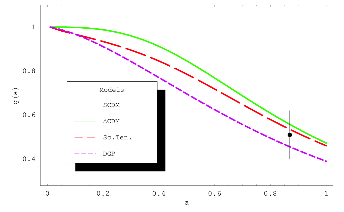
Figure 1: The growth rate in the (flat and $\Omega_{0m}=0.26$) $\Lambda$CDM (continuous line), Scalar-Tensor (long-dashed line) and DGP (short-dashed line) cases and a datapoint from the 2dFGRS $g(a=0.15)=0.51\pm 0.11$. The $\Lambda$CDM model is consistent with the current growth rate observations.

Alternatively, for the DGP modelDvali:2000rv ; Deffayet:2000uy we haveKoyama:2005kd

$$f(k,a)=(1+\frac{1}{3\beta})$$ (17)

with

$$\beta=1-\frac{H(a)}{H_{0}\sqrt{\Omega_{r_{c}}}}\left(1+\frac{a}{3}\frac{H^{\prime}(a)}{H(a)}\right)$$ (18)

where $r_{c}$ is the crossover scale beyond which the gravitational force follows the 5-dimensional $1/r^{3}$ behavior

$$\Omega_{r_{c}}\equiv 1/4r_{c}^{2}H_{0}^{2}$$ (19)

and $H(a)$ for the DGP model is defined through Koyama:2005kd

$$H_{DGP}(a)^{2}-\frac{H_{DGP}(a)}{r_{c}}=\frac{8\pi G}{3}\rho$$ (20)

Solving for $H_{DGP}(a)$, assuming flatness and in the case when we only have matter on the brane we get

$$\frac{H_{DGP}(a)}{H_{0}}=\sqrt{\Omega_{r_{c}}}+\sqrt{\Omega_{r_{c}}+\Omega_{0{\rm m}}a^{-3}}$$ (21)

where now

$$\Omega_{r_{c}}=\frac{1}{4}(1-\Omega_{0{\rm m}})^{2}$$ (22)

The detection of an $f(k,a)\neq 1$ from equation (14) would therefore be a ‘smoking gun’ signature of extended gravity theories. Such a detection could be made for example by using the form of $H(z)$ obtained from geometric tests in equation (14), solving for $D(a)$ in the context of general relativity ($f(k,a)=1$) and comparing with the observed $D(a)$ at various redshifts. If a statistically significant difference is found between the observed $D(a)$ and one predicted in the context of general relativity then this could be interpreted as evidence for extensions of general relativity.

There is currently an observational estimate of the growth rate defined as

$$g(a)\equiv\frac{aD^{\prime}(a)}{D(a)}$$ (23)

at a redshift $z=\frac{1}{a}-1=0.15$ from the 2dFGRSVerde:2001sf ; Hawkins:2002sg ; Wang:2004py . It is

$$g(z=0.15)=0.51\pm 0.11$$ (24)

and its derivation used the redshift distortion factor (see section III E). There will soon be better estimates coming from the SDSSTegmark:2003ud . In Fig. 1 we show the growth rate for the following flat models: a best fit ($\Omega_{0{\rm m}}=0.26$) $\Lambda$CDM model, a DGP ($\Omega_{0{\rm m}}=0.22$) model and a Scalar-Tensor model ($\xi=-0.2$ in equation (16) and $\Omega_{0{\rm m}}=0.26$). As demonstrated in Fig. 1 however, the large errorbars in the currently available datapoint of equation (24) can not distinguish the best fit $\Lambda$CDM model (flat $\Omega_{\Lambda}=0.74$) from other competing models. We therefore conclude that several different models including modified gravity models as well as $\Lambda$CDM are in agreement with current data.

Given the current uncertainties in the growth rate observations, it is important to uncover potential signatures of extended gravity theories in geometric observational methods. As discussed in the next section, a minimally coupled scalar field dark energy can not reproduce a $w(z)$ crossing the PDL ($w=-1$) for any scalar field potential (see however Ref Tsujikawa:2005cd for an interesting case). The simplest realistic theoretical model which can reproduce such crossing is a scalar-tensor extension of general relativity. Therefore, if such crossing is confirmed by geometric observations then this could be interpreted as an indication for extended gravity theories.

The structure of this paper is the following: In the next section we discuss the theoretical consequences emerging if the crossing of the PDL is confirmed by future observations. In section III we fit the parameterization Chevallier:2000qy ; Linder:2002et

$$w(z)=w_{0}+w_{1}\frac{z}{1+z}$$ (25)

to current data from various dark energy observational probes including the Gold SnIa sampleRiess:2004nr , the first year SNLS datasetAstier:2005qq , the 3-year WMAP CMB shift parameterSpergel:2006hy ; Wang:2006ts , the SDSS baryon acoustic peak (BAO)Eisenstein:2005su , the X-ray gas mass fraction in clustersAllen:2002sr ; Allen:2004cd and the linear growth rate of perturbations at $z=0.15$ as obtained from the 2dF galaxy redshift surveyVerde:2001sf ; Hawkins:2002sg , to investigate which of these probes currently favor crossing of the PDL and what are the priors required. Finally in section IV we conclude, summarize and outline future prospects of this work.

II Theoretical Implications of PDL Crossing

The simplest class of physically motivated models generalizing the cosmological constant and producing accelerated universe expansion are based on a simple evolving homogeneous scalar field $\Phi$ (quintessence Caldwell:1997ii ; Zlatev:1998tr ; Ratra:1987rm ) minimally coupled to gravity whose dynamics is determined by a potential $U(\Phi)$ and has a canonical kinetic term $\frac{1}{2}{\dot{\Phi}}^{2}$. It is easy to see however that this class of models can not reproduce a $w(z)$ crossing the PDL $w=-1$ for any potential $U(\Phi)$. Indeed, the equation of state $w$ for such models takes the form

$$w(z)=\frac{p_{X}}{\rho_{X}}=\frac{\frac{1}{2}{\dot{\Phi}}^{2}-U(\Phi)}{\frac{1}{2}{\dot{\Phi}}^{2}+U(\Phi)}$$ (26)

which approaches $w=-1$ in the limit of a small kinetic term but does not cross the PDL as long as ${\dot{\Phi}}^{2}>0$ for any sign of $U(\Phi)$. This result has been generalized by VikmanVikman:2004dc who showed that any minimally coupled scalar field with a generalized kinetic term also can not cross the PDL through a stable trajectory (see Refs Cannata:2006gd ; Andrianov:2005tm for an interesting exception involving however an arbitrary change of the kinetic term sign).

A simple ‘no go’ theoremAmendola:2006pc ; Kunz:2006wc can also be obtained for a general perfect barotropic fluid with conserved energy momentum tensor whose equation of state is of the form $p=p(\rho)$. Indeed energy conservation implies that

$${\dot{\rho}}=-3\frac{\dot{a}}{a}(\rho+p(\rho))$$ (27)

From this equation it follows that ${\dot{\rho}}\rightarrow 0$ as $p(\rho)\rightarrow-\rho$ or as $w=\frac{p}{\rho}\rightarrow-1$. By differentiating equation (27) with respect to time it is easy to see that ${\ddot{\rho}}\rightarrow 0$ as $w\rightarrow-1$ and similarly for all time derivatives of the density $\rho$ ie

$$\lim_{w\rightarrow-1}\frac{d^{n}\rho(t)}{dt^{n}}=0$$ (28)

for all $n$. Therefore, any fluid with equation of state of the form $p=p(\rho)$ can not cross the PDL. Instead it asymptotically approaches a constant energy density $\rho$ thus mimicking a cosmological constant. It should be stressed however that many scalar field models do not behave like barotropic ($p=p(\rho)$) fluids due to the dependence of $p$ and $\rho$ on two independent variables ${\dot{\Phi}}$ and $\Phi$ and therefore this proof is not equivalent to the proof that a minimally coupled scalar field can not cross the PDL.

Since the minimal theoretical approaches are unable to reproduce a PDL crossing we must turn to ‘non-minimal’ models to achieve such crossing. There are two main classes of such ‘non-minimal’ approaches: Either consider multiple component dark energyHu:2004kh ; Caldwell:2005ai ; Guo:2004fq ; Kunz:2006wc ; Zhao:2006mp ; Chimento:2006xu ; Stefancic:2005sp ; Wei:2006tn ; Zhao:2005bu ; Zhang:2006ck ; Li:2005fm ; Stefancic:2005cs (notice that higher derivative models and many non-barotropic fluids are effectively multi-component) with at least one phantom degree of freedom (eg scalar field with negative kinetic energy) or consider extensions of general relativity Boisseau:2000pr ; Esposito-Farese:2000ij ; Perivolaropoulos:2005yv ; Perrotta:1999am ; Aref'eva:2005fu ; Apostolopoulos:2006si ; Amendola:1999er ; McInnes:2005vp ; Gumjudpai:2005ry ; Onemli:2004mb ; Carroll:2004hc ; Nojiri:2005vv ; Nojiri:2006je ; Sahni:2002dx ; Alam:2005pb ; Chimento:2006ac ; Carroll:2004de ; Nojiri:2006ri ; Nojiri:2003ft . The phantom degrees of freedom of the former approach expressed by phantom fields are plagued by catastrophic UV instabilities since their energy is unbounded from below and allows vacuum decay through the production of high energy real particles and negative energy ghosts Cline:2003gs ; Buniy:2005vh ; Dubovsky:2005xd ; DeFelice:2006pg . On the other hand the general relativity extensions of the latter approach are severely constrained by local solar system and by cosmological observations but are well motivated theoretically.

To illustrate the multiple dark energy component approach to PDL crossing with scalar fields let’s consider a set of two coupled real scalar fields (quintessence $\Phi_{1}$ + phantom $\Phi_{2}$ : quintom dark energy Guo:2004fq ) with Lagrangian

$${\cal L}=\frac{1}{2}(\partial_{\mu}\Phi_{1})^{2}-\frac{1}{2}(\partial_{\mu}\Phi_{2})^{2}-U(\Phi_{1},\Phi_{2})$$ (29)

The effective pressure and energy density for a homogeneous system is

$$p = \frac{1}{2}{\dot{\Phi}_{1}}^{2}-\frac{1}{2}{\dot{\Phi}_{2}}^{2}-U(\Phi_{1},\Phi_{2})$$ (30)

$$\rho = \frac{1}{2}{\dot{\Phi}_{1}}^{2}-\frac{1}{2}{\dot{\Phi}_{2}}^{2}+U(\Phi_{1},\Phi_{2})$$ (31)

leading to the equation of state parameter

$$w=\frac{{\dot{\Phi}_{1}}^{2}-{\dot{\Phi}_{2}}^{2}-2U(\Phi_{1},\Phi_{2})}{{\dot{\Phi}_{1}}^{2}-{\dot{\Phi}_{2}}^{2}+2U(\Phi_{1},\Phi_{2})}$$ (32)

which crosses the PDL line when ${\dot{\Phi}_{1}}^{2}-{\dot{\Phi}_{2}}^{2}$ changes sign. This can easily be achieved with appropriate potentials and initial conditions.

The same approach may be illustrated by considering a mixture of multiple perfect fluids Hu:2004kh ; Stefancic:2005sp ; Caldwell:2005ai ; Stefancic:2005cs ; Nojiri:2005sr instead of scalar fields. Consider a mixture of two non-interacting fluids $(\rho_{1},p_{1},w_{1})$ and $(\rho_{2},p_{2},w_{2})$ with separately conserved energies and constant equation of state parameters $w_{1}$, $w_{2}$ with $w_{1}>-1$, $w_{2}<-1$. The equation of state parameter $w$ of the mixture is Kunz:2006wc

$$w=\frac{p}{\rho}=\frac{p_{1}+p_{2}}{\rho_{1}+\rho_{2}}=\frac{w_{1}\rho_{01}a^{-3(1+w_{1})}+w_{2}\rho_{02}a^{-3(1+w_{2})}}{\rho_{01}a^{-3(1+w_{1})}+\rho_{02}a^{-3(1+w_{2})}}$$ (33)

which interpolates between $w=w_{1}$ ($a<<1$) and $w=w_{2}$ ($a>>1$) thus crossing the PDL $w=-1$.

The requirement of phantom degrees of freedom which are plagued with several unattractive features Abramo:2005be ; Cline:2003gs ; Buniy:2005vh ; Dubovsky:2005xd ; DeFelice:2006pg ; Tsujikawa:2005aq (instabilities and lack of realistic prototypes) makes this class of approaches theoretically unattractive compared to the second class which is based on extensions of general relativity. Even though the latter are severely constrained observationally they are strongly motivated from the theoretical viewpoint. First it is clear that general relativity is an incomplete theory because it does not contain quantum mechanics and also it is plagued by singularities. Second, all theories that attempt to quantize gravity and/or unify it with other interactions require modifications of general relativity. For example, the string theory dilaton Gasperini:2002bn ; Copeland:2006wr field can be understood as the scalar field of an effective scalar-tensor theory in 4-dimensionsLevin:1994yw . Similarly, all Kaluza-Klein type theories which attempt to unify gravity with other interactions by utilizing compactified extra dimensions are described as effective scalar-tensor theories at low energiesPerivolaropoulos:2002pn ; Perivolaropoulos:2003we .

The simplest but very general (given its simplicity) extension of general relativity is expressed through scalar-tensor theories. In these theories Newton’s constant obtains dynamical properties expressed through the potential $F(\Phi)$. The dynamics are determined by the Lagrangian density Boisseau:2000pr ; Esposito-Farese:2000ij

$${\cal L}=\frac{F(\Phi)}{2}~{}R-\frac{1}{2}~{}g^{\mu\nu}\partial_{\mu}\Phi\partial_{\nu}\Phi-U(\Phi)+{\cal L}_{m}[\psi_{m};g_{\mu\nu}]\$$ (34)

where ${\cal L}_{m}[\psi_{m};g_{\mu\nu}]$ represents matter fields approximated by a pressureless perfect fluid. The function $F(\Phi)$ is observationally constrained as follows:

• $F(\Phi)>0$ so that gravitons carry positive energyEsposito-Farese:2000ij .

• $\frac{dF}{d\Phi}<10^{-5}$ from solar system observations will-bounds .

Assuming a homogeneous $\Phi$ and varying the action corresponding to (34) in a background of a flat FRW metric, we find the coupled system of generalized Friedman equations

$$3FH^{2} = \rho+\frac{1}{2}{\dot{\Phi}}^{2}-3H{\dot{F}}+U$$ (35)

$$-2F{\dot{H}} = \rho+p+{\dot{\Phi}}^{2}+{\ddot{F}}-H{\dot{F}}$$ (36)

where we have assumed the presence of a perfect fluid $(\rho=\rho_{m},p\simeq 0)$ playing the role of matter fields. Expressing in terms of redshift and eliminating the potential $U$ from equations (35), (36) we find Esposito-Farese:2000ij ; Perivolaropoulos:2005yv

$$\Phi^{\prime 2}=-F^{\prime\prime}-\left[(lnH)^{\prime}+\frac{2}{1+z}\right]F^{\prime}+2\frac{(lnH)^{\prime}}{1+z}F-$$

$$-3(1+z)\Omega_{0{\rm m}}\left(\frac{H_{0}}{H}\right)^{2}F_{0}>0$$ (37)

where ^′ denotes derivative with respect to redshift and $F_{0}$ is set to 1 in units of $\frac{1}{8\pi G_{N}}$ and corresponds to the present value of $F$. In the limit of minimal coupling ($F=1$) equation (37) becomes

$$\Phi_{mc}^{{}^{\prime}2}(H)=2\frac{(lnH)^{\prime}}{1+z}-3(1+z)\Omega_{0{\rm m}}(\frac{H_{0}}{H})^{2}>0$$ (38)

Using equation (6) it is easy to show that the inequality (38) is equivalent to $w(z)>-1$ which confirms the expectation that a minimally coupled scalar field is not consistent with PDL crossing. This constraint however is relaxed due to the allowed dynamical evolution of $F$ in equation (37) which may be written as

$$\Phi^{{}^{\prime}2}(F,H)=\Phi_{mc}^{{}^{\prime}2}(H)-\Delta(F,H)>0$$ (39)

where

$$\Delta(F,H)=F^{\prime\prime}+\left[(lnH)^{\prime}+\frac{2}{1+z}\right]F^{\prime}+2\frac{(lnH)^{\prime}}{1+z}(1-F)$$ (40)

Therefore, the constraint $\Phi_{mc}^{{}^{\prime}2}(H)>0$ is replaced in scalar-tensor theories by $\Phi_{mc}^{{}^{\prime}2}(H)>\Delta(F,H)$ and by choosing an $F$ such that $\Delta(F,H)<0$ a PDL crossing can be achieved.

The question to be addressed is the following: ‘Do observational constraints on $F$ allow $\Delta(F,H)<0$?’ The answer to that question is positive as may be easily seen by considering the present time ($z=0$) when the observational constraints Umezu:2005ee (and especially the solar system testswill-bounds ) are most stringent requiring $F^{\prime}(z)\simeq 0$ but placing no constraints on $F^{\prime\prime}(z=0)$. Setting $z=0$, $F=F_{0}=1$, $F^{\prime}=0$ in equation (37) we obtain

$$\left(\frac{H^{2}}{H_{0}^{2}}\right)^{\prime}(z = 0)>3\Omega_{0{\rm m}}+F^{\prime\prime}(z=0)$$

$$\implies w(z = 0)+1>\frac{F^{\prime\prime}(z=0)}{3(1-\Omega_{0{\rm m}})}$$ (41)

where we have used equation (6). Since there is no observational constraint on $F^{\prime\prime}(z=0)$ we can clearly pick $F^{\prime\prime}(z=0)<0$ allowing for $w(z=0)<-1$ and crossing the PDL.

There is a simple physical interpretation of the behavior required by $F$ in order to cross the PDL and lead to superacceleration ($w<-1$). Equation (40) implies that $\Delta(H,F)<0$ (and therefore $w<-1$) is favored for $F^{\prime\prime}<0$, $F^{\prime}<0$ and $F>1$. Since $F\sim G_{eff}^{-1}$ this behavior implies an effective Newton’s constant that increases with redshift ($G^{\prime\prime}_{eff}>0$, $G^{\prime}_{eff}>0$) and therefore decreases with time (${\ddot{G}}_{eff}<0$, ${\dot{G}}_{eff}<0$, $G_{eff}(t)>G_{eff}(t_{0})$) thus ‘helping’ the accelerating expansion induced by the potential $U$. This type of behavior was verified in a specific reconstruction example of $F(z)$, $U(z)$ in Ref. Perivolaropoulos:2005yv corresponding to an $H(z)-w(z)$ that crosses the PDL. It should be stressed however that any ansatz of $G_{eff}$ that is monotonic function of time, eg $G_{eff}(t)\sim t^{-\alpha}$ where $\alpha>0$, can lead to very tight constraints on the present values of $G^{\prime}_{eff}$ and $G^{\prime\prime}_{eff}$ using nucleosynthesis constraintsCopi:2003xd (but see also DeFelice:2005bx for a way to relax such constraints).

To summarize we have discussed two broad classes of models which can lead to crossing of the PDL: multicomponent dark energy with phantom components and extensions of general relativity. This is not an exhaustive classification but many of the left out models can be incorporated in the above classes. For example models of coupled quintessence where matter density Amendola:1999er is explicitly coupled to the scalar field causing acceleration may be shown to be conformally equivalent to scalar-tensor theories. Similarly, braneworld models Sahni:2002dx ; Apostolopoulos:2006si ; Aref'eva:2005fu ; Alam:2005pb ; Chimento:2006ac ; Bogdanos:2006pf ; Kofinas:2005hc can be classified as extended gravity theories. On the other hand in the multi-component class we could include models with a complex equation of stateArbey:2006it ; Kunz:2006wc , fermion models, scalar fields with higher derivativesLi:2005fm and vector field modelsZhao:2005bu . Of the two classes of theories discussed, the class of extended gravity theories is strongly motivated theoretically in contrast to the multicomponent class. Therefore, despite the observational constraints, extensions of general relativity is the prime candidate class of theories consistent with PDL crossing.

It is thus important to address the following questions:

• Do current cosmological data support a crossing of the PDL?

• What are the optimal observational strategies to confirm or exclude a PDL crossing with future observations?

The main goal of the next section is to address the first question using a broad sample of cosmological data. Previous studies Nesseris:2004wj have indicated that the SnIa data do not show a common trend regarding the crossing of the PDL. In particular, the analyses of the Gold SnIa dataset have indicated that a $w(z)$ that crosses the PDL is preferred over the $\Lambda$CDM parameter values at a level of almost $2\sigma$ Alam:2004jy ; Wang:2003gz ; Lazkoz:2005sp ; alam1 . On the other hand the SNLS dataset does not show such a trend Nesseris:2005ur ; Huterer:2004ch ; Santos:2006ja ; Jassal:2006gf ; Xia:2005ge and the $\Lambda$CDM parameter values are well within $1\sigma$ from the best fit parameter values. This raises the question as to what is the trend favored by the other than SnIa cosmological data. Do they favor the trend of PDL crossing indicated by the Gold dataset or do they favor a constant $w\simeq-1$ as indicated by SNLS? The main goal of the next section will be to address this question using the following cosmological data:

• The location of the CMB perturbation spectrum peaksSpergel:2006hy (shift parameterBond:1997wr ; Trotta:2004qj ; Melchiorri:2000px ).

• The measurement of the CMB acoustic scale at $z_{BAO}=0.35$ as indicated by the large scale structure correlation function of SDSS redshift survey (Baryon Acoustic Oscillations (BAO) peak) Eisenstein:2005su .

• The gas mass fraction of galaxy clusters $f_{gas}=\frac{M_{gas}}{M_{tot}}$ inferred from X-ray observations Allen:2004cd ; Allen:2002sr , which depends on the angular diameter distance $d_{A}$ to the cluster as $f_{gas}\sim d_{A}^{3/2}$.

• The linear growth factor $D(a)$ (eq. 13) as determined by the 2dF galaxy redshift surveyVerde:2001sf ; Hawkins:2002sg which can constrain $H(z)$ by using eq. (14) in the context of general relativity.

Using the above cosmological data we find the best fit form of $w(z)$ with $1\sigma$ errors in the context of the CPL parameterizationChevallier:2000qy ; Linder:2002et

$$w(a) = w_{0}+w_{1}(1-a)$$ (42)

$$w(z) = w_{0}+w_{1}\frac{z}{1+z}$$ (43)

We then compare this form with the corresponding best fits of both the Gold and the SNLS datasets to see which of the two trends is favored. The comparison is made for priors of $\Omega_{0m}$ in the range $0.2-0.3$.

III Observational of PDL Crossing

III.1 The SnIa datasets

The two most reliable and robust SnIa datasets existing at present are the Gold dataset Riess:2004nr and the Supernova Legacy Survey (SNLS) Astier:2005qq dataset. The Gold dataset compiled by Riess et. al. is a set of supernova data from various sources analyzed in a consistent and robust manner with reduced calibration errors arising from systematics. It contains 143 points from previously published data plus 14 points with $z>1$ discovered recently with the HST. The SNLS is a 5-year survey of SnIa with $z<1$. It has recently Astier:2005qq released the first year dataset. The SNLS has adopted a more efficient SnIa search strategy involving a ‘rolling search’ mode where a given field is observed every third or fourth night using a single imaging instrument thus reducing photometric systematic uncertainties. The published first year SNLS dataset consists of 44 previously published nearby SnIa with $0.015<z<0.125$ plus 73 distant SnIa ($0.15<z<1$) discovered by SNLS two of which are outliers and are not used in the analysis. The fact that in the two datasets a set of low-z SnIa is common to both samples could only lead to minor common systematics due to low redshift.

The above observations provide the apparent magnitude $m(z)$ of the supernovae at peak brightness after implementing correction for galactic extinction, K-correction and light curve width-luminosity correction. The resulting apparent magnitude $m(z)$ is related to the luminosity distance $D_{L}(z)$ through

$$m_{th}(z)={\bar{M}}(M,H_{0})+5log_{10}(D_{L}(z))$$ (44)

where in a flat cosmological model

$$D_{L}(z)=(1+z)\int_{0}^{z}dz^{\prime}\frac{H_{0}}{H(z^{\prime};a_{1},...,a_{n})}$$ (45)

is the Hubble free luminosity distance ($H_{0}d_{L}$), $a_{1},...,a_{n}$ are theoretical model parameters and ${\bar{M}}$ is the magnitude zero point offset and depends on the absolute magnitude $M$ and on the present Hubble parameter $H_{0}$ as

$${\bar{M}} = M+5log_{10}(\frac{H_{0}^{-1}}{Mpc})+25=$$ (46)

$$= M-5log_{10}h+42.38$$

The parameter $M$ is the absolute magnitude which is assumed to be constant after the above mentioned corrections have been implemented in $m(z)$.

The data points of the Gold dataset are given after the corrections have been implemented, in terms of the distance modulus

$$\mu^{G}_{obs}(z_{i})\equiv m^{G}_{obs}(z_{i})-M$$ (47)

The SNLS dataset however also presents for each point, the stretch factor $s$ used to calibrate the absolute magnitude and the rest frame color parameter $c$ which mainly measures host galaxy extinction by dust. Thus, the distance modulus in this case depends apart from the absolute magnitude $M$, on two additional parameters $\alpha$ and $\beta$ defined from

$$\mu_{obs}^{SNLS}=m_{obs}^{SNLS}(z_{i})-M+\alpha(s_{i}-1)-\beta c_{i}$$ (48)

which are fit along with the theoretical parameters using a recursive procedure.

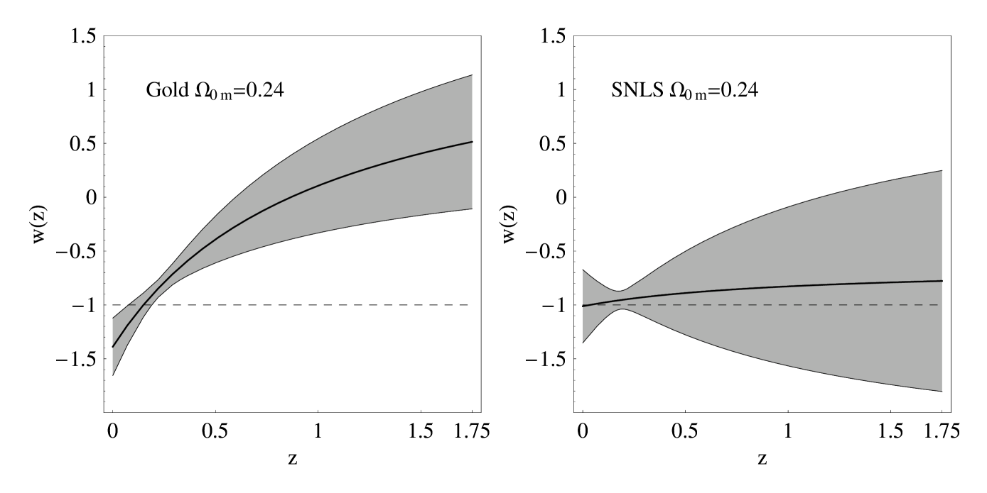
Figure 2: The best fit form of $w(z)$ for the Gold and SNLS datasets for a prior of $\Omega_{0m}=0.24$ along with the $1\sigma$ errors (shaded region).

The theoretical model parameters are determined by minimizing the quantity

$$\chi^{2}_{SnIa}(\Omega_{0{\rm m}},w_{0},w_{1})=\sum_{i=1}^{N}\frac{(\mu_{obs}(z_{i})-\mu_{th}(z_{i}))^{2}}{\sigma_{\mu\;i}^{2}+\sigma_{int}^{2}+\sigma_{v\;i}^{2}}$$ (49)

where $N=115$ for SNLS ($\chi^{2}_{SNLS}$), $N=157$ for the Gold dataset ($\chi^{2}_{Gold}$), $\sigma_{\mu\;i}^{2}$, $\sigma_{int}^{2}$ and $\sigma_{v\;i}^{2}$ are the errors due to flux uncertainties, intrinsic dispersion of SnIa absolute magnitude and peculiar velocity dispersion respectively. These errors are assumed to be gaussian and uncorrelated. The theoretical distance modulus is defined as

$$\mu_{th}(z_{i})\equiv m_{th}(z_{i})-M=5log_{10}(D_{L}(z))+\mu_{0}$$ (50)

where

$$\mu_{0}=42.38-5log_{10}h$$ (51)

and $\mu_{obs}$ is given by (47) and (48) for the Gold and SNLS datasets respectively.

The steps we followed for the minimization of (49) for the Gold and SNLS datasets are described in detail in Refs Nesseris:2004wj ; Nesseris:2005ur ; Nesseris:2006jc . The form of $H(z)$ used in (45), (50) is obtained by using the CPL parameterization (43) and leads to

$$H^{2}(z) = H_{0}^{2}[\Omega_{0m}(1+z)^{3}+$$ (52)

$$+ (1-\Omega_{0m})(1+z)^{3(1+w_{0}+w_{1})}e^{\frac{-3w_{1}z}{(1+z)}}]$$

The best fit form of $w(z)$ for the Gold and first year SNLS datasets is shown in Fig. 2 for a prior of $\Omega_{0{\rm m}}=0.24$ along with the $1\sigma$ errorsnumerics (shaded region). Even though the two fits are consistent at the $1\sigma$ level it is clear that the Gold sample mildly favors a crossing of the PDL at $z\simeq 0.25$ while no such trend appears for the SNLS data. This trend difference could be attributed to three factors

• Statistical errors

• Systematic errors

• Different redshift ranges (Gold $0<z<1.7$, SNLS $0<z<1$).

The third possibility has been excluded in Ref. Nesseris:2005ur where a truncated version of the Gold sample with $(0<z<1)$ was found to show even stronger trend for crossing the PDL than the full Gold sample. Given this apparent difference in trends between the Gold and the SNLS datasets the following question arises: ‘Which (if any) of the two trends do other cosmological probes of dark energy favor?’

III.2 The CMB shift parameter

A particularly accurate and deep geometrical probe of dark energy is the angular scale of the sound horizon at the last scattering surface as encoded in the location $l_{1}^{TT}$ of the first peak of the CMB temperature perturbation spectrum. By measuring the angular scale $\theta_{1}^{TT}\sim 1/l_{1}^{TT}$ of the last scattering sound horizon and calculating its comoving scale $r_{s}(z_{dec})$ independently from CMB physics, the sound horizon angular diameter distance $d_{A}(z_{rec})$ can be obtained assuming flatness as

$$d_{A}(z_{rec})=\frac{r_{s}(z_{rec})}{\theta_{1}^{TT}}=\frac{1}{1+z_{rec}}\int_{0}^{z_{rec}}\frac{dz}{H(z)}$$ (53)

thus providing a useful constraint on $H(z)$. To eliminate the model dependence involved in the calculation of the sound horizon scale an (approximately) model independent parameter can be defined by dividing the measured angle $\theta_{1}^{TT}\sim 1/l_{1}^{TT}$ by the corresponding angle $\theta_{1}^{{}^{\prime}TT}$ of a reference model. This parameter is known as the ‘shift parameter’.

The shift parameter is defined as Bond:1997wr ; Efstathiou:1998xx ; Trotta:2004qj ; Melchiorri:2000px

$$R=\frac{l_{1}^{{}^{\prime}TT}}{l_{1}^{TT}}$$ (54)

where $l_{1}^{TT}$ is the temperature perturbation CMB spectrum multipole of the first acoustic peak. In the definition of $R$, $l_{1}^{TT}$ corresponds to the model (with fixed $\Omega_{0m}$, $\Omega_{0b}$ and $h$) characterized by the shift parameter and $l_{1}^{{}^{\prime}TT}$ a reference flat SCDM model ($\Omega^{\prime}_{0m}=1$) with the same $\omega_{m}\equiv\Omega_{0m}h^{2}$, $\omega_{b}=\Omega_{0b}h^{2}$ as the original model.

The location $l_{1}^{TT}$ of the first acoustic peak can be connected with the angular diameter distance $d_{A}$ to the last scattering surface and with the sound horizon $r_{s}$ at the last scattering surface ($z=z_{rec}$) as follows Efstathiou:1998xx ; Hu:2000ti :

$$l_{1}^{TT}=l_{A}(d_{A},r_{s})(1-\psi(\omega_{m},\omega_{b}))$$ (55)

where

$$l_{A}(d_{A},r_{s}) \equiv \frac{\pi}{\theta_{1}^{TT}}$$ (56)

$$\theta_{1}^{TT} \equiv \frac{r_{s}(z_{rec})}{d_{A}(z_{rec})}$$ (57)

and the phase shift parameter $\psi(\omega_{m},\omega_{b})\simeq 0.27$ Hu:2000ti depends weakly on cosmological parameters. The sound horizon $r_{s}$ and the angular diameter distance $d_{A}$ depend on the Hubble expansion history (at early and late times respectively) as follows:

$$r_{s} = a_{rec}\int_{0}^{a_{rec}}\frac{c_{s}(a)da}{a^{2}H(a)}=$$ (58)

$$= a_{rec}\int_{0}^{a_{rec}}\frac{c_{s}(a)da}{\Omega_{0{\rm m}}^{1/2}}\left[\frac{\Omega_{r}h^{2}}{\Omega_{0{\rm m}}h^{2}}+a\right]^{-1/2}$$

where $c_{s}(a)$ is the sound velocity which at decoupling ($a=a_{rec}$) is

$$c_{s}^{2}(a_{rec})=\frac{\delta p}{\delta\rho}=\frac{1}{3}\frac{1}{1+\frac{3\Omega_{b}}{4\Omega_{r}}a_{rec}}$$ (59)

and

$$d_{A}(z)=\frac{a_{rec}}{H_{0}\sqrt{\Omega_{k}}}sin\left[H_{0}\sqrt{\Omega_{k}}\int_{0}^{z_{rec}}\frac{dz^{\prime}}{H(z^{\prime})}\right]$$ (60)

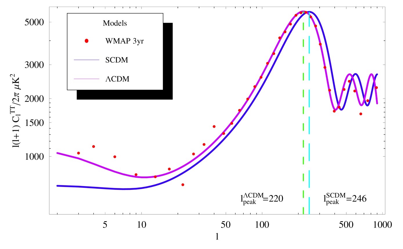
Figure 3: Derivation of the shift parameter: The 3-year WMAP binned data along with a theoretical flat $\Lambda$CDM model ($\omega_{m}=0.14,\omega_{b}=0.022,h=0.72$) and a SCDM model with ($\omega_{m}=0.14,\omega_{b}=0.022,h=0.37$). For the $\Lambda$CDM the first peak is at $l_{1}^{TT}=220$ while for the SCDM model at $l_{1}^{{}^{\prime}TT}=246$.

For the reference model SCDM we have

$$d^{\prime}_{A}(z^{\prime}_{rec}) = \frac{a_{rec}}{H_{0}}\int_{0}^{z_{rec}}\frac{dz^{\prime}}{\left[\Omega_{0{\rm m}}^{\prime}(1+z)^{3}+\Omega_{r}^{\prime}(1+z)^{4}\right]^{1/2}}=$$

$$= \frac{2a_{rec}}{H_{0}}\left[(a^{\prime}_{eq}+1)^{1/2}-(a^{\prime}_{{rec}}+a^{\prime}_{eq})^{1/2}\right]=$$

$$= \frac{2a_{rec}}{H_{0}}\left[(\Omega_{r}^{\prime}+1)^{1/2}-(a^{\prime}_{{rec}}+\Omega_{r}^{\prime})^{1/2}\right]$$

$$\equiv \frac{2a_{rec}}{H_{0}}q(\Omega_{r}^{\prime},a^{\prime}_{rec})$$

Using equations (55)-(III.2) it is easy to show that

$$R = \frac{l_{1}^{{}^{\prime}TT}}{l_{1}^{TT}}=\frac{l_{A}^{{}^{\prime}}(1-\psi^{\prime})}{l_{A}(1-\psi)}=$$ (62)

$$= \frac{r_{s}}{r^{\prime}_{s}}\frac{d^{\prime}_{A}(z^{\prime}_{rec})}{d_{A}(z_{rec})}=\frac{2}{\Omega_{0{\rm m}}^{1/2}}\frac{q(\Omega_{r}^{\prime},a_{rec})}{\chi(z)}$$

where

$$\chi(z)\equiv\int_{0}^{z}\frac{H_{0}dz^{\prime}}{H(z^{\prime})}$$ (63)

and we have assumed flatness and used the fact that $\psi=\psi^{\prime}$ (since $\omega_{b}=\omega^{\prime}_{b}$ and $\omega_{m}=\omega_{m}^{\prime}$) and $a_{rec}(\omega_{b},\omega_{m})=a^{\prime}_{rec}(\omega^{\prime}_{b},\omega^{\prime}_{m})$ Hu:2000ti . The main advantage of using the shift parameter instead of just the value of $l_{1}^{TT}$ is that it is weakly dependent on parameters other than geometry ($H(z)$). The dependence on other parameters enters through $\Omega_{0{\rm m}}^{-1/2}$ and through $q(\Omega_{r}^{\prime},a_{rec})=q(\omega_{r}/h^{\prime 2},a_{rec}(\omega_{m},\omega_{b}))$ where $\omega_{r}\equiv\Omega_{r}h^{2}\simeq 2.47\cdot 10^{-5}$, $h^{\prime 2}=\omega_{m}$ and Hu:2000ti $z_{rec}=\frac{1}{a_{rec}}-1=1048(1+0.00124\omega_{b}^{-0.738})(1+g_{1}\omega_{m}^{g_{2}})$ where $g_{1}=0.0783\omega_{b}^{-0.238}(1+39.5\omega_{b}^{0.763})^{-1}$ and $g_{2}=0.560(1+21.1\omega_{b}^{1.81})^{-1}$. Notice that the weak dependence of the shift parameter on $\omega_{m}$, $\omega_{b}$ through $q(\omega_{m},\omega_{b})$ has not been explicitly demonstrated in previous studies Wang:2006ts . Instead, the shift parameter is usually expressed as

$$R^{\prime}=\frac{2}{\Omega_{0{\rm m}}^{1/2}\chi(z_{rec})}$$ (64)

or equivalently as ${\bar{R}}=\Omega_{0{\rm m}}^{1/2}\chi(z_{rec})$ thus omitting the correction factor $q(\omega_{m},\omega_{b})$. For fixed $\Omega_{0{\rm m}}=0.27$, $\Omega_{b}=0.043$ and $0.5\leq h\leq 0.9$, $q(\omega_{m},\omega_{b})$ remains in the range $0.964\leq q\leq 0.968$ and therefore the dependence on the Hubble parameter introduced by $q$ is very weak.

The main disadvantage of the shift parameter is that in order to evaluate it using its definition (54) for a given CMB perturbation spectrum we need not only the location of the first peak $l_{1}^{TT}$ but also the location of the reference model (SCDM) peak. For an accurate result, the latter requires running a Boltzmann code like CAMB Lewis:1999bs with $\Omega_{0{\rm m}}^{\prime}=1$, $\omega^{\prime}_{m}=\omega_{m}$, $\omega^{\prime}_{b}=\omega_{b}$ and evaluating the location of the first peak $l_{1}^{{}^{\prime}TT}$. This procedure is illustrated in Fig. 3 where we show the 3-year WMAP data along with a theoretical fit obtained for $(\omega_{m},\omega_{b},h)=(0.14,0.022,0.72)$ assuming flat $\Lambda$CDM. The first peak for the best fit model is obtained at $l_{1}^{TT}=220\pm 0.8$ while for the reference flat SCDM model with $(\omega_{m},\omega_{b},h)=(0.14,0.022,0.37)$ (leading to $\Omega_{0{\rm m}}=1$) we have $l_{1}^{{}^{\prime}TT}=246$ (see Fig. 3). We thus obtain

$$R=\frac{l_{1}^{{}^{\prime}TT}}{l_{1}^{TT}}=1.123\pm 0.03$$ (65)

Using now (62) and (64) with $q=0.965$ we find

$${\bar{R}}\equiv\Omega_{0{\rm m}}^{1/2}\chi(z_{rec})=1.71\pm 0.05$$ (66)

This result is consistent but slightly different from that of Ref. Wang:2006ts which used MCMC chains to obtain ${\bar{R}}$ from WMAP3 as

$${\bar{R}}=1.70\pm 0.03$$ (67)

In what follows we adopt the result of eq. (67) to obtain the best fit $w(z)$.

Even though the shift parameter incorporates most of the geometrical information of the CMB spectrum the following question can be raised: ‘How much of the CMB spectrum geometrical information is left out of the shift parameter?’ To answer this question we proceed in two steps: First we consider the CPL parameterization and construct CMB spectra (using a modified version of CAMBLewis:1999bs ) varying $H(z)$ with fixed ${\bar{R}}$ and other CMB parameters (see Fig. 4 and Table 1). The constructed CMB spectra are practically identical for all values of $l$ except low $l$ ($l\buildrel<\over{\sim}50$) where there are minor differences due to the ISW effect Pogosian:2005ez ; Melchiorri:2002ux . These CMB spectra differences can not be observationally distinguished due to the large cosmic variance errors that dominate at low $l$.

The temperature anisotropy due to the ISW effect is given by an integral over the time variation of the gravitational potential traversed by the photons coming from the last scattering surfacePogosian:2005ez

$$\Theta_{l}(k,\eta_{0})=(2l+1)\int_{\eta_{rec}}^{\eta_{0}}d\eta e^{-\tau}\left[2{\dot{\Phi}}(k,\eta)\right]j_{l}(k(\eta_{0}-\eta))$$ (68)

where the overdot indicates conformal time derivative, $\Theta\equiv\frac{\Delta T}{T}$ and the integral is taken over the line to the last scattering surface. Due to the integral over the oscillating Bessel functions $j_{l}$, the dominant contribution to the CMB anisotropy is on large scales (low $l$). The gravitational potential $\Phi(k,\eta)$ (metric fluctuation of FRW background) may be shown (using the Einstein equations) to

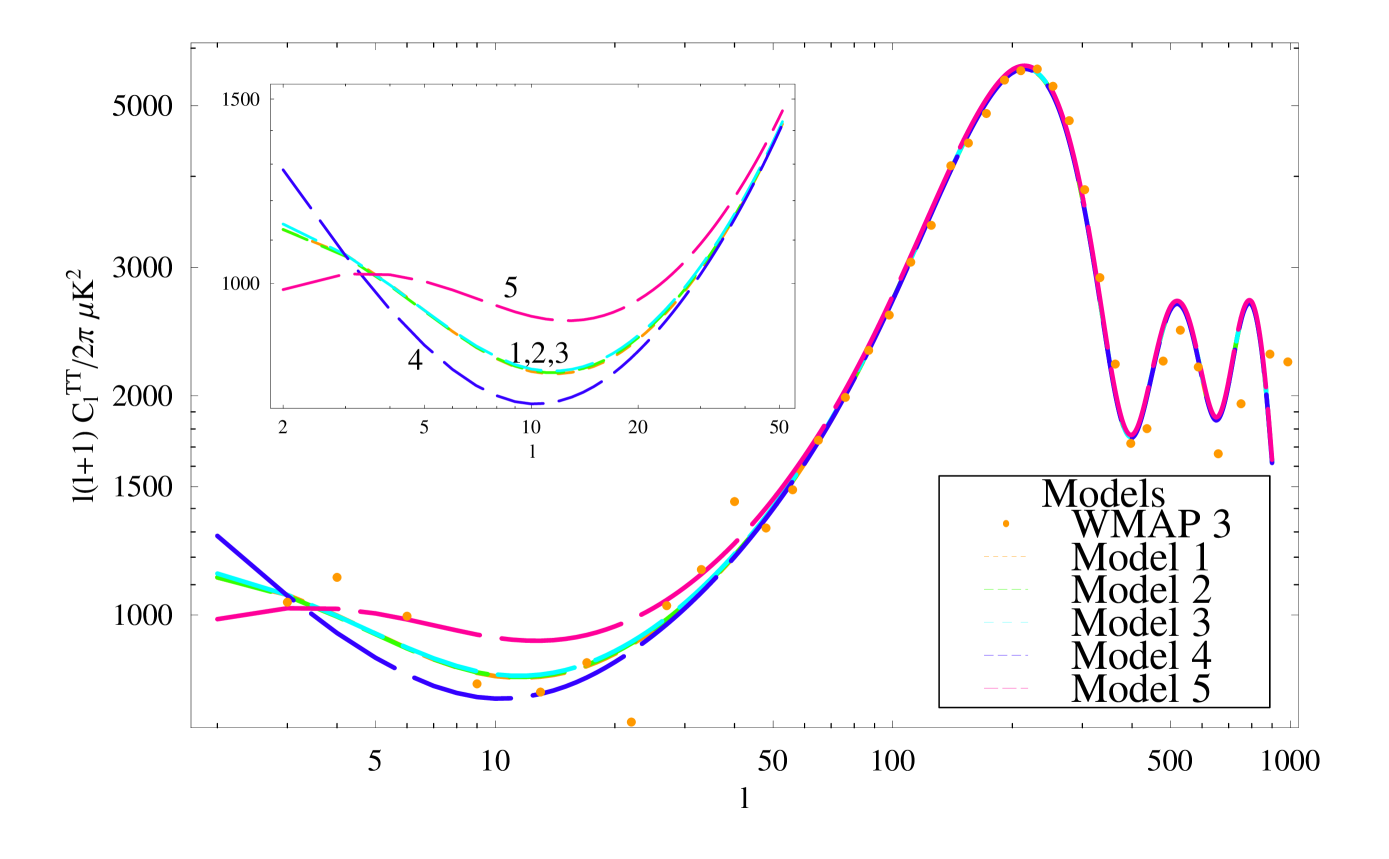
Figure 4: Theoretical CMB spectra for the CPL parameterization for five models that have fixed ${\bar{R}}=1.70$ and other parameters (see text and Table 1). Models (1,2,3) with identical $\Omega_{0{\rm m}}$ and ${\bar{R}}$ but different $w(z)$ have practically identical spectrum for all $l$ (identical ISW effect). The ISW effect for fixed ${\bar{R}}$ changes only due to variations of $\Omega_{0{\rm m}}$ (models 4, 5)!

obey a Poisson equation which in a flat universe is of the form

$$k^{2}\Phi(k,\eta)=4\pi Ga^{2}\delta\rho$$ (69)

where $\delta\rho$ is the density perturbation. In a flat, matter dominated universe we have $\frac{\delta\rho}{\rho}\sim a\implies\delta\rho\sim a^{-2}$ which implies (due to (69)) that ${\dot{\Phi}}=0$ and there is no ISW effect. However, in the presence of dark energy, the evolution of perturbations is delayed at late times $\left(\frac{\delta\rho}{\rho}<\left(\frac{\delta\rho}{\rho}\right)_{i}a\right)$ and therefore ${\dot{\Phi}}\neq 0$ leading to a non-zero ISW effect. The ISW effect therefore measures the growth rate of perturbations at late times or its deviation from the flat matter dominated rate $\frac{\delta\rho}{\rho}\sim a$.

Table 1: Parameters for the 5 models of Fig. 4.

Models	$\Omega_{0m}$	$w_{0}$	$w_{1}$	$h$
Model 1	0.27	-0.8	-0.123	0.725
Model 2	0.27	-0.9	0.196	0.725
Model 3	0.27	-1.0	0.497	0.725
Model 4	0.14	-1.7	-1.061	0.998
Model 5	0.50	-0.3	-0.064	0.533

An interesting feature of Fig. 4 is that if we keep ${\bar{R}}$ and $\Omega_{0{\rm m}}$ fixed while varying $H(z)$, the ISW effect appears to be unchanged! In contrast, if we keep ${\bar{R}}$ fixed while varying $\Omega_{0{\rm m}}$ and $H(z)$ ($\rho_{X}(z)$), the ISW effect changes indicating that perhaps there is not much more information in the ISW effect about the dark energy density evolution than that included in the shift parameter ${\bar{R}}$. This is also demonstrated in Fig. 5 where we show the growth of perturbations $D(a)$ for the five models of Fig. 4. Clearly, those models which have identical ISW effect

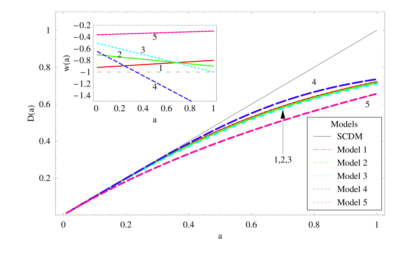
Figure 5: The growth of perturbations $D(a)$ for the five models of Fig. 4 along with the corresponding forms of $w(a)$. Those models (1,2,3) which have identical ISW effect (same $\Omega_{0{\rm m}}$ and ${\bar{R}}$ but different $H(z)-w(z)$) also have very similar growth of perturbations even though the dark energy density evolution is quite different.

(same $\Omega_{0{\rm m}}$ and ${\bar{R}}$ but different $H(z)$) also have very similar growth of perturbations even though the dark energy density evolution is quite different!

It should be stressed that whatever information about dark energy is encoded in the ISW effect, this information can not be extracted directly from the temperature perturbation CMB spectrum (due to the large cosmic variance errors at low $l$) but only using alternative methods like CMB cross correlationPogosian:2005ez with large scale structure or CMB polarizationCooray:2002cb .

The measurement of the shift parameter (equation (66)) allows us to add an important term to the $\chi^{2}$ of equation (49) obtained with SnIa. This term is of the form

$$\chi^{2}_{CMB}(\Omega_{0{\rm m}},w_{0},w_{1})=\frac{({\bar{R}}(\Omega_{0{\rm m}},w_{0},w_{1})-1.70)^{2}}{0.03^{2}}$$ (70)

This term is very important in constraining evolving dark energy models for two reasons:

1. The shift parameter has a very low relative error (few percent)

2. The integral over $H(z)$ extends to high redshift ($z_{rec}\simeq 1089$). Therefore, minor modifications of $H(z)$ can be very ‘costly’ in $\chi^{2}$ exactly due to this term.

Another similar term is obtained from the imprint of the last scattering sound horizon on the large scale structure correlation function.

III.3 The Baryon Acoustic Peak

The large scale correlation function measured from the luminous red galaxies spectroscopic sample of the SDSS (Sloan Digital Sky Survey) Eisenstein:2005su includes a clear peak at about $100h^{-1}Mpc$. This peak was identified with the expanding spherical wave of baryonic perturbations originating from acoustic oscillations at recombination. The comoving scale of this shell at recombination is about 150Mpc in radius. The identification of the comoving scale where the correlation peak was observed with the acoustic horizon at recombination requires the appropriate form of the cosmological model $H(z)$ in converting from the observed angles-redshift to correlation function distances. An accurate determination of the best fit $H(z)$ would therefore correspond to using a general model or parameterization of $H(z)$ to convert from the observed angles-redshifts to correlation function distances and then vary these parameters until the observed Baryon Acoustic Oscillation (BAO) peak coincides with the expected value from CMB physics.

A simplified version of this approach was used in Refs. Eisenstein:2005su , Blake:2003rh . It involves the use of a fiducial $\Lambda$CDM $H(z)$ model to construct the correlation function from the observed angles-redshifts and identify the distance scale $r_{peak}$ where the BAO peak appears. Comparing this value of $r_{peak}$ with the expected value $r^{\prime}_{peak}$ from CMB physics would require a scale shift by a factor $\alpha$: $r^{\prime}_{peak}=\alpha r_{peak}$. This factor $\alpha$ can be approximated as the ratio of the required characteristic distance scale $D_{V}(z_{BAO})$ of the survey with mean redshift $z_{BAO}$ (obtained with the correct $H(z)$) over the distance scale $D_{V}^{\Lambda CDM}(z_{BAO})$ corresponding to the fiducial $\Lambda$CDM model

$$\alpha=\frac{r^{\prime}_{peak}}{r_{peak}}=\frac{D_{V}(z_{BAO})}{D_{V}^{\Lambda CDM}(z_{BAO})}$$ (71)

The characteristic distance scale of the redshift survey with typical redshift $z_{s}$ can be connected to $H(z)$ as follows: Consider a spherical shell (Fig. 6) of comoving radius R. Let $z$ be the redshift corresponding to the sphere (points C and D) as viewed by an observer at O and $\Delta z$ the redshift difference between A and B.

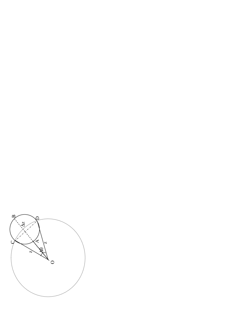
Figure 6: A spherical shell in redshift space.

If we measure the angular scale $\Delta\theta$, the redshifts $z$ and $\Delta z$, then given a cosmological model $H(z)$, the comoving scales CD and AB may be evaluated from the flat FRW metric asAlcock:1979mp

$$CD=x\Delta\theta=\Delta\theta\int_{t_{i}}^{t_{0}}\frac{dt}{a}=\frac{\Delta\theta}{H_{0}}\int_{0}^{z}\frac{dz}{E(z)}$$ (72)

where $E(z)\equiv H(z)/H_{0}$ and

$$AB=\Delta x=\frac{\Delta t}{a}=\frac{1}{H_{0}}\frac{\Delta z}{E(z)}$$ (73)

Generalizing the above to a deformed sphere ($AB\neq CD$) we may associate an approximate single scale to the sphere as Eisenstein:2005su

$$D_{V}(z) = \left[\left(\frac{CD}{\Delta\theta}\right)^{2}(AB)\right]^{1/3}=$$ (74)

$$= \left[\left(\frac{1}{H_{0}}\int_{0}^{z}\frac{dz}{E(z)}\right)^{2}\frac{1}{H_{0}}\frac{\Delta z}{E(z)}\right]^{1/3}$$

where $CD/\Delta\theta$ is the comoving angular diameter distance. We also want this scale to be representative of the whole sample (fiducial scale for SDSS $z_{BAO}=0.35$) so we allow the sphere to extend from the observer to ($A\rightarrow O$) to $z\simeq 0.35$ ($z_{BAO}\simeq 0.35$) and therefore $\Delta z\simeq z_{BAO}\simeq 0.35$. For low redshift samples (like $z_{BAO}=0.35$), the dilation scale $D_{V}(z)$ can be assumed to encode all the information required for converting redshift to distance. By demanding that the scale of the peak of the correlation function coincides with the acoustic scale (which is predicted by simple physics (see eq. (58)) and depends on $\Omega_{0{\rm m}}h^{2}$) it has been shown Eisenstein:2005su that

$$D_{V}(0.35)=1370\pm 64Mpc$$ (75)

for $\Omega_{0{\rm m}}h^{2}=0.130\pm 0.010$. A dimensionless and independent of $H_{0}$ version of the dilation scale $D_{V}$ is

$$A \equiv D_{V}(0.35)\frac{\sqrt{\Omega_{0{\rm m}}H_{0}^{2}}}{z_{BAO}}=$$ (76)

$$= \Omega_{0{\rm m}}^{1/2}E(z_{BAO})^{-1/3}[\frac{1}{z_{BAO}}\int_{0}^{z_{1}}\frac{dz^{\prime}}{E(z^{\prime})}]^{2/3}=$$

$$= 0.469\pm 0.017$$

This parameter has been used extensively in constraining dark energy models (see eg Alam:2005pb ; Alcaniz:2006ay ) and it will also be used in what follows.

The measurement of the parameter $A$ (equation (76)) permits the addition of one more term in the $\chi^{2}$ of equations (49), (70) to be minimized with respect to $H(z)$ model parameters. This term is

$$\chi^{2}_{BAO}(\Omega_{0{\rm m}},w_{0},w_{1})=\frac{(A(\Omega_{0{\rm m}},w_{0},w_{1})-0.469)^{2}}{0.017^{2}}$$ (77)

III.4 The Cluster Baryon Gas Mass Fraction

The baryon gas mass fraction for a range of redshifts can also be used to constrain cosmological models $H(z)$. The basic assumption underlying this method is that the baryon gas mass fraction in clusters Arnaud:2005vq ; Allen:2002sr ; Allen:2004cd :

$$f_{gas}=\frac{M_{b-gas}}{M_{tot}}$$ (78)

is constant, independent of redshift and is related to the global fraction of the universe $\frac{\Omega_{b}}{\Omega_{0{\rm m}}}$ in a simple way. This relation may be written as

$$b\frac{\Omega_{b}}{\Omega_{0{\rm m}}}=\frac{M_{b}}{M_{tot}}=(1+\alpha)\frac{M_{b-gas}}{M_{tot}}=(1+\alpha)f_{gas}$$ (79)

where $b$ is a bias factor suggesting that the baryon fraction in clusters is slightly lower than for the universe as a whole. Also $1+\alpha$ is a factor taking into account the fact that the total baryonic mass in clusters consists of both X-ray gas and optically luminous baryonic mass (stars), the latter being proportional to the former with proportionality constant $\alpha\simeq 0.19\sqrt{h}$ Allen:2004cd . Assuming now that the hot gas in a cluster follows a spherically symmetric isothermal model i.e.

$$n_{e}=n_{e0}(1+\frac{r^{2}}{r_{c}^{2}})^{-3\beta/2}$$ (80)

where $\beta$ is a constant, $n_{e}$ is the electron number density and $n_{e0}$, $r_{c}$ are the central electron density and the core radius respectively, it is straightforward to show that Sasaki:1996ss ; Pen:1996sb

$$M_{gas}(<R)=B(T_{e},R/r_{c},\beta)r_{c}^{3/2}L_{X}(<R)^{1/2}$$ (81)

In eq. (81) $T_{e}$ is the electron temperature, $L_{X}(<R)$ is the bolometric luminosity within radius $R$ and $B$ is a constant independent of cosmological parameters. The quantities $r_{c}$, $L_{X}(<R)$ are obtained from the observed angular core radius $\theta_{c}$ and the observed apparent luminosity within $\theta$ ($l_{X}(<\theta)$) as

$$L_{X}(<R) = 4\pi d_{L}(z)^{2}l_{X}(<\theta)$$ (82)

$$r_{c} = \theta_{c}d_{A}(z)$$ (83)

$$R = \theta d_{A}(z)$$ (84)

where $d_{L}(z)$ and $d_{A}(z)$ are the luminosity and diameter distances which depend on the cosmological model $H(z)$ as

$$d_{L}(z)=(1+z)^{2}d_{A}(z)=(1+z)\int_{0}^{z}\frac{dz^{\prime}}{H(z^{\prime})}$$ (85)

in the context of a flat cosmology. From eqs (81)-(85) we obtain

$$M_{gas}(<R)=C(\theta_{c},\theta,l_{X},z)d_{A}(z)^{5/2}$$ (86)

where all cosmological model dependence is encoded in $d_{A}(z)$ while C depends on observables characterizing each cluster ($\theta_{c}$, $l_{X}(<\theta)$,$T_{e}$,$z$).

Table 2: Cluster data from Ref. Allen:2004cd .

$z_{i}$	$f_{gas,i}$	$\sigma_{gas,i}^{2}$
0.078	0.189	0.011
0.088	0.184	0.011
0.143	0.167	0.019
0.188	0.169	0.011
0.206	0.180	0.015
0.208	0.137	0.018
0.240	0.163	0.009
0.252	0.164	0.012
0.288	0.149	0.017
0.313	0.169	0.010
0.314	0.175	0.023
0.324	0.177	0.018
0.345	0.173	0.019
0.352	0.189	0.025
0.363	0.159	0.017
0.391	0.159	0.024
0.399	0.177	0.017
0.450	0.155	0.019
0.451	0.137	0.009
0.461	0.129	0.019
0.461	0.156	0.034
0.494	0.094	0.025
0.539	0.135	0.011
0.686	0.155	0.018
0.782	0.100	0.016
0.892	0.114	0.021

Similarly, the total cluster mass within $R$ $M_{tot}(<R)$ may be obtained assuming that the intracluster mass is in hydrostatic equilibrium as

$$M_{tot}(<R)=D\;R=D\;\theta\;d_{A}(z)$$ (87)

where $D$ is independent of cosmological model parameters. From eqs (86) and (87) we find that

$$f_{gas}=\frac{M_{gas}(<R)}{M_{tot}(<R)}=\frac{C}{D\theta}d_{A}(z)^{3/2}\equiv Qd_{A}(z)^{3/2}$$ (88)

where $Q$ depends only on individual cluster observables. Assume now that the quantities $Q_{i}$ $(i=1,...,N)$ have been obtained for an observed sample of $N$ clusters at redshifts $z_{i}$. Using eqs. (79) and (88) we have

$$b\frac{\Omega_{b}}{\Omega_{0{\rm m}}}=(1+\alpha)f_{gas}(z_{i})=(1+\alpha)Q_{i}d_{A}(z_{i})^{3/2}$$ (89)

Define now

$$f_{gas}^{SCDM}(z_{i})\equiv Q_{i}\;d_{A}^{SCDM}(z_{i})^{3/2}$$ (90)

where $d_{A}^{SCDM}(z_{i})$ is the angular diameter distance corresponding to SCDM (flat $\Omega_{0{\rm m}}=1$) used as a reference model. Solving (90) for $Q_{i}$ and substituting in eq. (89) we find

$$f_{gas}^{SCDM}(z_{i})\equiv\frac{b}{1+\alpha}\frac{\Omega_{b}}{\Omega_{0{\rm m}}}\left(\frac{d_{A}^{SCDM}(z_{i})}{d_{A}(z_{i})}\right)^{3/2}$$ (91)

Since now $f_{gas}^{SCDM}$ is known observationally (see eq. (90)) we can use eq. (91) to find the best fit $d_{A}(z_{i})$ and therefore the corresponding best fit cosmological model. We use the 26 cluster data for $f_{gas}^{SCDM}(z_{i})$ published in Ref. Allen:2004cd and minimize $\chi_{CBF}^{2}$ (Cluster Baryon Fraction) defined as

$$\chi^{2}_{CBF}(\Omega_{0{\rm m}},w_{0},w_{1})\equiv\sum_{i=1}^{26}\frac{(f_{gas}^{SCDM}(z_{i})-f_{gas,i})^{2}}{\sigma_{f_{gas,i}}^{2}}$$ (92)

where $f_{gas}^{SCDM}(z_{i})$ is given by eq. (91) and the observed $f_{gas,i}$, $\sigma_{gas,i}^{2}$ used in our analysis are shown in Table 2. We treat $\frac{b}{1+\alpha}\frac{\Omega_{b}}{\Omega_{0{\rm m}}}$ as a nuisance parameter and we marginalize over it as follows: Define $\lambda\equiv\frac{b}{1+\alpha}\frac{\Omega_{b}}{\Omega_{0{\rm m}}}$ then

$$f_{gas}^{SCDM}(z_{i})=\lambda\cdot\left(\frac{d_{A}^{SCDM}(z_{i})}{d_{A}(z_{i})}\right)^{3/2}\equiv\lambda\cdot\tilde{f}_{gas}^{SCDM}(z_{i})$$ (93)

and eq. (92) after expanding with respect to $\lambda$ becomes

$$\chi^{2}_{CBF}\equiv\lambda^{2}A-2\lambda B+C$$ (94)

where

$$A = \sum_{i=1}^{N}\frac{\tilde{f}_{gas}^{SCDM}(z_{i})^{2}}{\sigma_{f_{gas,i}}^{2}}$$

$$B = \sum_{i=1}^{N}\frac{\tilde{f}_{gas}^{SCDM}(z_{i})\cdot f_{gas,i}}{\sigma_{f_{gas,i}}^{2}}$$

$$C = \sum_{i=1}^{N}\frac{f_{gas,i}^{2}}{\sigma_{f_{gas,i}}^{2}}$$ (95)

Equation (94) has a minimum for $\lambda=B/A$ at

$$\tilde{\chi}^{2}_{CBF}\equiv C-B^{2}/A$$ (96)

which is independent of $\lambda$. The $\tilde{\chi}^{2}_{CBF}$ of eq. (96) is the one actually used in our analysis. It should be pointed out however that the relative errors of these datapoints are more than $10\%$ and therefore variations of $H(z)$ with given $\Omega_{0{\rm m}}$ prior affect the value of $\chi_{CBF}^{2}$ much less than SnIa, CMB and BAO data.

III.5 Linear Growth Rate at z=0.15

The 2dF galaxy redshift survey (2dFGRS) has measured the two point correlation function at an effective redshift of $z_{s}=0.15$. This correlation function is affected by systematic differences between redshift space and real space measurements due to the peculiar velocities of galaxies. Such distortions are expressed through the redshift distortion parameter $\beta$ which connects the power spectrum in redshift space $P_{s}({\vec{k}})$ with the true galaxy power spectrum $P_{g}(k)$ as

$$P_{s}({\vec{k}})=(1+\beta\mu^{2})^{2}P_{g}(k)$$ (97)

where $\mu=\cos\theta$ and $\theta$ is the angle between ${\vec{k}}$ and the line of sight. The parameter $\beta$ can be observationally determined from the observed power spectrum (or its Fourier transform, the correlation function) in redshift space and may be shown to be connected to the growth factor $D(a)$ at the effective redshift of the power spectrum asHamilton:1997zq

$$\beta=\frac{g}{b}$$ (98)

where

$$g\equiv a\frac{dD(a)/da}{D(a)}$$ (99)

and $b$ is the bias factor ($b\equiv\frac{\delta_{g}}{\delta}$) which connects the overdensity in galaxies $\delta_{g}$ with the matter overdensity $\delta$. The derivation of eq. (98) may be sketched as followsHamilton:1997zq : The radial position of a galaxy with low redshift $z$ and no peculiar velocity is approximated by

$$\chi(z)=\frac{z}{H_{0}}$$ (100)

and therefore its redshift space position vector is

$${\vec{x}}_{s}=\frac{z}{H_{0}}(\sin\theta\cos\phi,\sin\theta\cos\phi,\cos\theta)$$ (101)

Due to gravitational effects however, galaxies have peculiar velocities ${\vec{v}}$ which affect the redshift $z$ as $z=H_{0}x+{\vec{v}}\cdot{\hat{x}}$ where ${\hat{x}}$ is the line of sight direction. Therefore, the true comoving distance $x$ to the galaxy is connected to the redshift inferred distance as

$$\frac{z}{H_{0}}\equiv x_{s}=x+\frac{{\vec{v}}\cdot{\hat{x}}}{H_{0}}$$ (102)

Our goal is to connect the galaxy overdensity in redshift space $\delta_{s}=\frac{\delta\rho_{s}({\vec{x}}_{s})}{{\bar{\rho}}}$ with the corresponding galaxy overdensity $\delta_{g}=\frac{\delta\rho_{g}(x)}{{\bar{\rho}}}$ in real space.

The number of galaxies in a spatial region is the same, independent of the coordinate system i.e.

$$n_{s}({\vec{x}}_{s})d^{3}x_{s}=n({\vec{x}})d^{3}x$$ (103)

or

$${\bar{n}}(1+\delta_{s})={\bar{n}}(1+\delta_{g})\frac{dx}{dx_{s}}\frac{x^{2}}{x_{s}^{2}}$$ (104)

where ${\bar{n}}$ is the average number density of galaxies. Assuming low velocities and focusing on modes $kx>>1$ we obtain from eqs (102) and (104)

$$\delta_{s}({\vec{x}})=\delta_{g}({\vec{x}})-\frac{\partial}{\partial x}(\frac{{\vec{v}}(x)\cdot{\hat{x}}}{H_{0}})$$ (105)

By Fourier transforming eq. (105) and expressing the peculiar velocity in terms of the mass overdensity $\delta$ using the continuity equation

$$a\frac{d\delta}{dt}+ikv=0$$ (106)

which impliesHamilton:1997zq

$${\vec{v}}(k,a)=\frac{igaH\delta(k,a){\vec{k}}}{k^{2}}$$ (107)

we find (for low redshifts $z<<1$)

$${\tilde{\delta}}_{s}({\vec{k}})=\delta_{g}(k)+g\mu^{2}\delta(k)$$ (108)

where $\mu=\cos\theta={\hat{k}}\cdot{\hat{x}}$ and $g$ is defined by eq (99). We now use the bias factor $b\equiv\frac{\delta_{g}}{\delta}$ to write eq. (108) as

$${\tilde{\delta}}_{s}({\vec{k}})=(1+\frac{g}{b}\mu^{2})\delta_{g}(k)$$ (109)

which leads to eqs (97) and (98).

The parameter $\beta=\frac{g}{b}$ may be measured from redshift surveys by measuring $P_{s}({\vec{k}})$ and expanding both sides of eq. (97) in Legendre polynomials ${\cal P}_{l}(\mu)$Hamilton:1997zq :

$$P_{s}({\vec{k}}) = P_{s}^{(0)}(k){\cal P}_{0}(\mu)+P_{s}^{(2)}(k){\cal P}_{2}(\mu)+P_{s}^{(4)}(k){\cal P}_{4}(\mu)=$$ (110)

$$= (1+\beta\mu^{2})^{2}P_{g}(k)=[(1+\frac{2}{3}\beta+\frac{1}{5}\beta^{2}){\cal P}_{0}(\mu)+$$

$$+ (\frac{4}{3}\beta+\frac{4}{7}\beta^{2}){\cal P}_{2}(\mu)+\frac{8}{35}\beta^{2}{\cal P}_{4}(\mu)]P_{g}(k)$$

Therefore one way to measure $\beta$ is to use the measured quadrupole $P_{s}^{(2)}(k)$ and monopole $P_{s}^{(0)}(k)$ as

$$\frac{P_{s}^{(2)}(k)}{P_{s}^{(0)}(k)}=\frac{\frac{4}{3}\beta+\frac{4}{7}\beta^{2}}{1+\frac{2}{3}\beta+\frac{1}{5}\beta^{2}}$$ (111)

which leads to the value of $\beta$ and (if the bias is determined) to the value of $g$ at the effective redshift of the redshift survey.

The correlation function (the Fourier transform of the galaxy power spectrum) can also be used instead of the power spectrum to obtain $\beta$ using a very similar method as the one described above. Such a method was used along with others in Ref. Verde:2001sf to find

$$\beta=0.49\pm 0.09$$ (112)

at the effective redshift of $z=0.15$ of the 2dF redshift survey. This result may now be combined with the linear bias parameter

$$b=1.04\pm 0.11$$ (113)

obtained from the skewness induced in the bispectrum of the 2dFRGSHawkins:2002sg by linear biasing to find the growth factor $g$ at $z=0.15$ as

$$g=a\frac{D^{\prime}(a)}{D(a)}|_{z=0.15}=b\cdot\beta=0.51\pm 0.11$$ (114)

Such a result can in principle be used in combination with eq. (14) with $f(k,a)=1$ to constrain $H(z)$ in the context of general relativity or, if $H(z)$ is determined by other observations, to determine the function $f(k,a)$ in eq. (14) thus providing a robust test of alternative gravity theories.

Under the assumption of general relativity, the measurement of the Perturbations Growth Rate (PGR) $g(z=0.15)$ can be used to add one more term to $\chi^{2}$ as

$$\chi^{2}_{PGR}(\Omega_{0{\rm m}},w_{0},w_{1})=\frac{(g(\Omega_{0{\rm m}},w_{0},w_{1})-0.51)^{2}}{0.11^{2}}$$ (115)

where $g(\Omega_{0{\rm m}},w_{0},w_{1})$ is obtained by solving equation (14) with $f(k,a)=1$ and initial conditions $D(a)\simeq a$ for $a\simeq 0$.

Notice however that the large relative error of this datapoint (about $25\%$) makes the contribution of $\chi^{2}_{LSS}$ rather insensitive to variations of $H(z)$. If however future observations reduce the relative error of this measurement it is potentially very important as it is a dynamical test capable of distinguishing between general relativity and extended gravity theories along the lines discussed in section I.

III.6 Cosmological Data and PDL Crossing

In order to identify the trends encoded in the current cosmological data with respect to dark energy evolution and in particular PDL crossing we group the data in three categories:

1. SnIA Gold sample

2. SnIA SNLS

3. Other Dark Energy Probes (ODEP) that include the CMB, BAO, Cluster Baryon Fraction (CBF) and Perturbations Growth Rate (PGR) at $z=0.15$

The corresponding $\chi^{2}$ to be minimized for each category are

• $\chi^{2}_{Gold}(\Omega_{0{\rm m}},w_{0},w_{1})$ (equation (49))

• $\chi^{2}_{SNLS}(\Omega_{0{\rm m}},w_{0},w_{1})$ (equation (49))

• Using equations (70), (77), (92) and (115) we have

  $$\chi_{ODEP}^{2}\equiv\chi^{2}_{CMB}+\chi^{2}_{BAO}+\chi^{2}_{CBF}+\chi^{2}_{PGR}$$ (116)

In order to identify the dependence of the resulting best fits on the $\Omega_{0{\rm m}}$ prior used we have not marginalized over $\Omega_{0{\rm m}}$. Instead we have fixed $\Omega_{0{\rm m}}$ and considered two cases ($\Omega_{0{\rm m}}=0.2$ and $\Omega_{0{\rm m}}=0.3$). The range between the two cases includes the current best fit value of $\Omega_{0{\rm m}}$ based on WMAP and SDSS which isTegmark:2006az $\Omega_{0{\rm m}}=0.24\pm 0.02$.The errors of the best fit $w(z)$ were obtained using the covariance matrix (see eg press92 ; Alam:2004ip ). The best fit form of $w(z)$ for each dataset category is shown in Fig. 7 for both $\Omega_{0{\rm m}}=0.2$ and $\Omega_{0{\rm m}}=0.3$. The corresponding $\chi^{2}$ contours in the $w_{0}-w_{1}$ parameter space is shown in Fig. 8.

The following comments can be made based on our results summarized in Figs. 7 and 8:

• The Gold dataset mildly favors dynamically evolving dark energy crossing the PDL at $z\simeq 0.2$ over the cosmological constant while the SNLS does not.

• Dark energy probes other than SnIa mildly favor crossing of the PDL for low values of $\Omega_{0{\rm m}}$ ($\Omega_{0{\rm m}}\buildrel<\over{\sim}0.25$) while for $\Omega_{0{\rm m}}\simeq 0.3$ this trend is significantly reduced.

• The best probes of dark energy with currently existing data, other than SnIa are the CMB shift parameter and the BAO peak.

The last point emerges by plotting the third column of Figs. 7, 8 utilizing only CMB and BAO data. Such plots are practically unchanged compared to those of Figs. 7, 8.

An important issue that needs to be addressed before closing this section is the issue of systematics introduced by using a particular parametrization to fit the cosmological expansion history. There is no doubt that the best fit forms to a given dataset may differ significantly between different parametrizations. However, the particular property of PDL crossing at best fit has been shown to be a robust feature for several $H(z)-w(z)$ parametrizations in the context of the Gold dataset provided that these parametrizations allow for PDL crossing. This was demonstrated in Ref Lazkoz:2005sp (Fig. 1) where we compared the best fit forms of a wide range parametrizations to the Gold dataset.

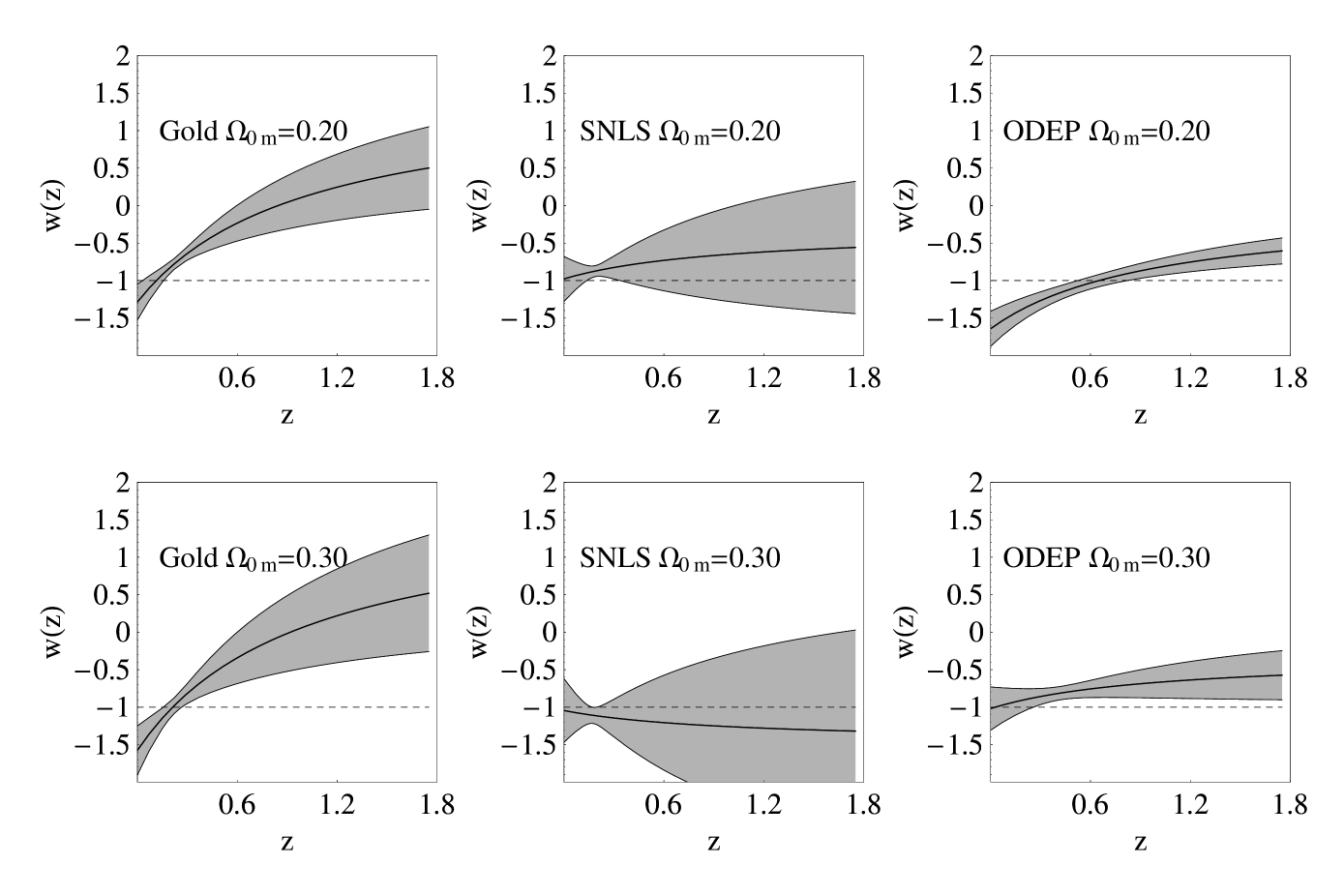
Figure 7: The best fit form of $w(z)$ for each dataset category for both $\Omega_{0m}=0.2$ and $\Omega_{0m}=0.3$ along with the $1\sigma$ errors (shaded region). The categories are: Gold dataset (column 1), SNLS (column 2) and Other Dark Energy Probes (ODEP column 3).

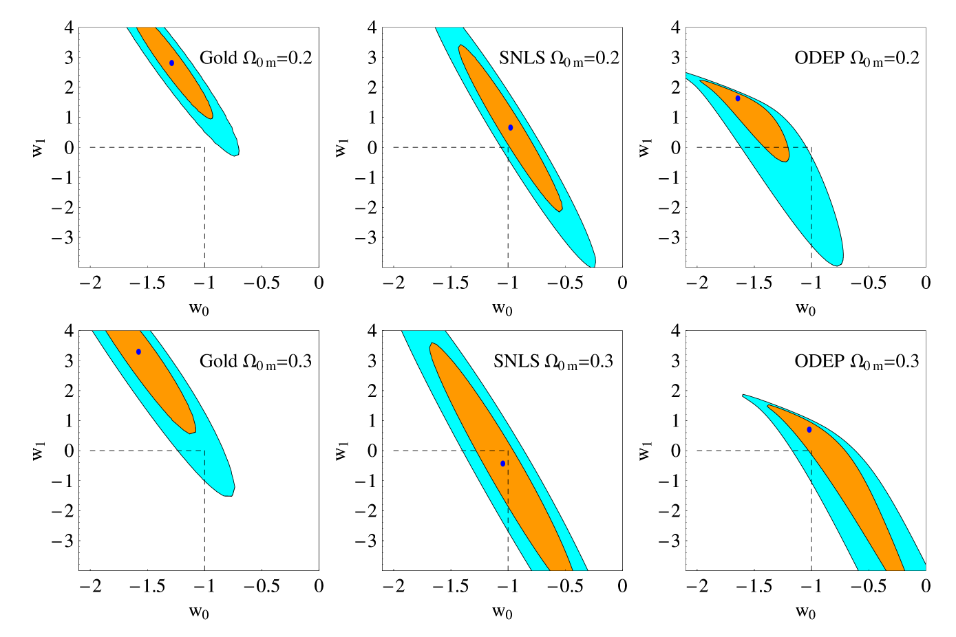
Figure 8: The $68\%$ and $95\%$ $\chi^{2}$ confidence contours in the $w_{0}-w_{1}$ parameter space for each dataset category for both $\Omega_{0m}=0.2$ and $\Omega_{0m}=0.3$. Notice that for the SNLS dataset $\Lambda$CDM is within the $1\sigma$ region.

In that paper it was demonstrated that even though the high redshift properties at best fit were different for each parametrization, the low redshift properties and in particular the PDL crossing which appears at $z\simeq 0.2$ are very robust and consistent among the different parametrizations. This robustness can also be checked in the context of Other Dark Energy Probes. We have fitted three different $H(z)$ parametrizations to the ODEP along the lines of Ref. Lazkoz:2005sp . We found that the best fit forms for each parametrization indicate crossing of the PDL for low $\Omega_{0{\rm m}}$ but in this case there is a spread in the redshift range of crossing in the range $0.4<z<1.8$. In view of the very broad redshift covering ($0<z<1089$) of the dominant probe of this class which is the CMB shift parameter, the above spread in the crossing range is not a significant indicator of systematics.

Another source of systematics that deserves attention is the robustness of our results shown in Figs 7 and 8 with respect to the theory of gravity considered. Modified gravity theories are expected to affect dynamical tests of dark energy (which depend on the way the metric couples to energy momentum tensor) but not geometrical tests which detect directly the evolution of the FRW-metric. Tests based on standard candles (SnIa) and standard rulers (CMB shift parameter, BAO peak and X-ray gas mass fraction) are geometric tests and we do not expect modified gravity theories to have a direct effect on them. For example even though the CMB spectrum will vary in modified gravity theories (in particular its ISW part), its geometric features like the first peak location depend only on the background metric and act as a standard ruler measuring directly the integral of H(z).

On the other hand the test based on the growth rate of perturbations at $z=0.15$ would give a different form for $H(z)$ in the context of modified gravity theories (see Fig. 1). This effect however would hardly modify our results of Figs. 7, 8 because the $1\sigma$ error of the perturbations growth contributions to $\chi^{2}$ is much larger that the geometrical tests contributions. In fact we have found that even if we completely ignore the dynamical test contribution to Figs. 7, 8 these figures remain practically unchanged. We should stress however that there is an indirect effect of modified gravity theories on SnIa standard candles. The possibility of a time varying Newtons constant would induce a variation of the Chandrasekhar mass and lead to a variation of the SnIa absolute luminosity. This effect was studied in Ref. Nesseris:2006hp for an evolving Newton’s constant consistent with nucleosynthesis and solar system bounds. It was found that the effect is negligible for current SnIa data but may have to be taken into account for future data with SNAP level accuracy.

It is therefore clear that even though currently available dark energy probes agree on the fact that the dark energy equation of state $w(z)$ is close to $-1$ there is no universal trend with respect to the evolution properties of dark energy and the existing trends appear to depend on the value of $\Omega_{0{\rm m}}$ prior considered.

IV Conclusion-Outlook

We have pointed out the importance of identifying observational signatures that could distinguish between dark energy and extended gravity theories as possible origins of the accelerating expansion of the universe. The crossing of the PDL $w=-1$ can be identified as such a signature based on a geometrical dark energy probe. We have noted that the simplest theoretically motivated class of theories that is consistent with such crossing is the class of extended gravity theories. A representative example of this class of theories includes scalar-tensor theories.

Even though there are currently no clear observational indications for a PDL crossing, there are probes of accelerating expansion that mildly favor such crossing over a constant equation of state. These probes include the Gold SnIa dataset for any reasonable prior for $\Omega_{0{\rm m}}$ as well as the combination of other than SnIa probes (CMB, BAO, Clusters Baryon Fraction and growth rate of perturbations) with a low $\Omega_{0{\rm m}}$ prior ($\Omega_{0{\rm m}}\buildrel<\over{\sim}0.25$). On the other hand a non-evolving $w\simeq-1$ appears to be favored by the SNLS first year data.

Another (perhaps more robust) signature which could rule out dark energy in favor of extended gravity theories is obtained by utilizing the measurement of the growth rate of perturbations at various redshifts. This test utilizes a ‘dynamical’ (as opposed to ‘geometrical’) dark energy probe. We have demonstrated how can this measurement be used to distinguish between the two classes of theories. We have also pointed out that current 2dFGRS data are consistent with $\Lambda$CDM in the context of general relativity and require no extended gravity theory.

We have also discussed the ISW effect as another potentially interesting dynamical probe of dark energy which is sensitive to the growth rate of perturbations at recent redshifts. We have demonstrated that in the context of general relativity and for fixed shift parameter ${\bar{R}}$ and fixed $\Omega_{0{\rm m}}$ the ISW effect on the CMB power spectrum and the growth factor of perturbations $D(a)$ appear to be insensitive to modifications of the dark energy equation of state. Degeneracies of the CMB power spectrum with fixed shift parameter ${\bar{R}}$ have been discussed previously Melchiorri:2002ux but in those cases $\Omega_{0{\rm m}}$ was varied simultaneously with a $w(z)=w_{0}=const$ to keep ${\bar{R}}$ constant. Thus, the large scale part of the CMB spectrum was seen to vary in those studies due to the variation of $D(a)$ (ISW effect). The degeneracy observed here can be used as an additional observational discriminator between general relativity and extended gravity theories. For example if the ISW effect is found to differ from the expected form obtained by the measured shift parameter ${\bar{R}}$ and $\Omega_{0{\rm m}}$ then this could be viewed as an indication of extensions of general relativity. A more quantitative form of this argument is an interesting potential extension of this work.Modifications of the ISW effect are expected for example in theories predicting a time varying Newton’s constant. In particular in Ref. Sawicki:2005cc it was shown that in the DGP model at late times, perturbations enter a DGP regime in which the effective value of Newton’s constant increases as the background density diminishes. This leads to a suppression of the ISW effect, bringing DGP gravity into slightly better agreement with WMAP data than conventional LCDM.

The PDL crossing viewed as a geometrical signature of extended gravity assumes the non-existence of phantom degrees of freedom which is a reasonable assumption in view of the theoretical problems of such degrees of freedom. On the other hand the dynamical signature (growth rate of perturbations) assumes that the dark energy perturbations can be ignored on sub-horizon scales and can not mimic the effects of modified gravity theories expressed through the function $f(k,a)$ (equation (14)). These assumptions make it important to identify further types of observational signatures that can be used in combination with the above, providing more robust tests that could distinguish between the two classes of theories.

Numerical Analysis: Our numerical analysis was performed using a Mathematica code implementing $\chi^{2}$ fitting of multiple dark energy probes and a modified version of CAMB allowing for a dynamical $w(z)$ using the CPL parametrization. All the codes and data along with detailed instructions are available at http://leandros.physics.uoi.gr/pdl-cross/pdl-cross.htm

References

- (1) Riess A et al., 1998 Astron. J. 116 1009; Perlmutter S J et al., 1999 Astroph. J. 517 565; Bull.Am.Astron.Soc29,1351(1997); Tonry, J L et al., 2003 Astroph. J. 594 1; Barris, B et al., 2004 Astroph. J. 602 571; Knop R et al., 2003 Astroph. J. 598 102;
- (2) A. G. Riess et al. [Supernova Search Team Collaboration], Astrophys. J. 607, 665 (2004) [arXiv:astro-ph/0402512].
- (3) P. Astier et al., Astron. Astrophys. 447, 31 (2006) [arXiv:astro-ph/0510447].
- (4) D. J. Eisenstein et al. [SDSS Collaboration], Astrophys. J. 633, 560 (2005) [arXiv:astro-ph/0501171].
- (5) S. W. Allen, R. W. Schmidt and A. C. Fabian, Mon. Not. Roy. Astron. Soc. 334, L11 (2002) [arXiv:astro-ph/0205007].
- (6) S. W. Allen, R. W. Schmidt, H. Ebeling, A. C. Fabian and L. van Speybroeck, Mon. Not. Roy. Astron. Soc. 353, 457 (2004) [arXiv:astro-ph/0405340].
- (7) D. N. Spergel et al., arXiv:astro-ph/0603449.
- (8) L. Verde et al., Mon. Not. Roy. Astron. Soc. 335, 432 (2002) [arXiv:astro-ph/0112161].
- (9) H. Hoekstra, H. K. C. Yee and M. D. Gladders, Astrophys. J. 577, 595 (2002) [arXiv:astro-ph/0204295].
- (10) V. Sahni and A. A. Starobinsky, Int. J. Mod. Phys. D 9, 373 (2000) [arXiv:astro-ph/9904398].
- (11) E. J. Copeland, M. Sami and S. Tsujikawa, arXiv:hep-th/0603057.
- (12) T. Padmanabhan, arXiv:astro-ph/0603114.
- (13) L. Perivolaropoulos, arXiv:astro-ph/0601014.
- (14) N. Straumann, Mod. Phys. Lett. A 21, 1083 (2006) [arXiv:hep-ph/0604231].
- (15) J. P. Uzan, arXiv:astro-ph/0605313.
- (16) V. Sahni and A. Starobinsky, arXiv:astro-ph/0610026.
- (17) P. J. E. Peebles and B. Ratra, Rev. Mod. Phys. 75, 559 (2003) [arXiv:astro-ph/0207347].
- (18) S. M. Carroll, Living Rev. Rel. 4, 1 (2001) [arXiv:astro-ph/0004075].
- (19) S. Weinberg, arXiv:astro-ph/0005265.
- (20) R. R. Caldwell, R. Dave and P. J. Steinhardt, Phys. Rev. Lett. 80, 1582 (1998) [arXiv:astro-ph/9708069].
- (21) I. Zlatev, L. M. Wang and P. J. Steinhardt, Phys. Rev. Lett. 82, 896 (1999) [arXiv:astro-ph/9807002].
- (22) B. Ratra and P. J. E. Peebles, Phys. Rev. D 37, 3406 (1988).
- (23) T. D. Saini, S. Raychaudhury, V. Sahni and A. A. Starobinsky, Phys. Rev. Lett. 85, 1162 (2000) [arXiv:astro-ph/9910231]; D. Huterer and M. S. Turner, Phys. Rev. D 64, 123527 (2001) [arXiv:astro-ph/0012510].
- (24) B. Boisseau, G. Esposito-Farese, D. Polarski and A. A. Starobinsky, Phys. Rev. Lett. 85, 2236 (2000) [arXiv:gr-qc/0001066].
- (25) S. Nojiri, S. D. Odintsov and M. Sami, Phys. Rev. D 74, 046004 (2006) [arXiv:hep-th/0605039].
- (26) V. Sahni and Y. Shtanov, JCAP 0311, 014 (2003) [arXiv:astro-ph/0202346].
- (27) L. P. Chimento, R. Lazkoz, R. Maartens and I. Quiros, arXiv:astro-ph/0605450.
- (28) S. M. Carroll, A. De Felice, V. Duvvuri, D. A. Easson, M. Trodden and M. S. Turner, Phys. Rev. D 71, 063513 (2005) [arXiv:astro-ph/0410031].
- (29) C. Deffayet, Phys. Lett. B 502, 199 (2001) [arXiv:hep-th/0010186].
- (30) G. Esposito-Farese and D. Polarski, Phys. Rev. D 63, 063504 (2001) [arXiv:gr-qc/0009034].
- (31) D. F. Torres, Phys. Rev. D 66, 043522 (2002) [arXiv:astro-ph/0204504].
- (32) R. Gannouji, D. Polarski, A. Ranquet and A. A. Starobinsky, arXiv:astro-ph/0606287.
- (33) L. Perivolaropoulos, arXiv:astro-ph/0504582.
- (34) E. Bertschinger, arXiv:astro-ph/0604485.
- (35) Y. Wang and P. Mukherjee, arXiv:astro-ph/0604051.
- (36) S. Sasaki, PASJ, 48, L119 (1996)
- (37) E. Hawkins et al., Mon. Not. Roy. Astron. Soc. 346, 78 (2003) [arXiv:astro-ph/0212375].
- (38) P. Fischer et al. [SDSS Collaboration], Astron. J. 120, 1198 (2000) [arXiv:astro-ph/9912119].
- (39) S. Borgani and L. Guzzo, Nature, 409, 39 (2001).
- (40) M. J.Rees and D. W. Sciama, Nature 217 511 (1968); R. G. Crittenden and N. Turok, Phys. Rev. Lett. 76, 575 (1996); L. Pogosian, P. S. Corasaniti, C. Stephan-Otto, R. Crittenden and R. Nichol, Phys. Rev. D 72, 103519 (2005) [arXiv:astro-ph/0506396].
- (41) M. Tegmark et al. [SDSS Collaboration], Phys. Rev. D 69, 103501 (2004) [arXiv:astro-ph/0310723].
- (42) M. Tegmark et al. [SDSS Collaboration], Astrophys. J. 606, 702 (2004) [arXiv:astro-ph/0310725].
- (43) H. F. Stabenau and B. Jain, arXiv:astro-ph/0604038.
- (44) G. R. Dvali, G. Gabadadze and M. Porrati, Phys. Lett. B 484, 112 (2000) [arXiv:hep-th/0002190].
- (45) K. Koyama and R. Maartens, JCAP 0601, 016 (2006) [arXiv:astro-ph/0511634].
- (46) Y. Wang and M. Tegmark, Phys. Rev. Lett. 92, 241302 (2004) [arXiv:astro-ph/0403292].
- (47) S. Tsujikawa, Phys. Rev. D 72, 083512 (2005) [arXiv:astro-ph/0508542].
- (48) M. Chevallier and D. Polarski, Int. J. Mod. Phys. D 10, 213 (2001) [arXiv:gr-qc/0009008].
- (49) E. V. Linder, Phys. Rev. Lett. 90, 091301 (2003) [arXiv:astro-ph/0208512].
- (50) A. Vikman, Phys. Rev. D 71, 023515 (2005) [arXiv:astro-ph/0407107].
- (51) F. Cannata and A. Y. Kamenshchik, arXiv:gr-qc/0603129.
- (52) A. A. Andrianov, F. Cannata and A. Y. Kamenshchik, Phys. Rev. D 72, 043531 (2005) [arXiv:gr-qc/0505087].
- (53) L. Amendola, private communication (2006).
- (54) M. Kunz and D. Sapone, arXiv:astro-ph/0609040.
- (55) W. Hu, Phys. Rev. D 71, 047301 (2005) [arXiv:astro-ph/0410680].
- (56) R. R. Caldwell and M. Doran, arXiv:astro-ph/0501104.
- (57) Z. K. Guo, Y. S. Piao, X. M. Zhang and Y. Z. Zhang, arXiv:astro-ph/0410654; B. Feng, X. L. Wang and X. M. Zhang, Phys. Lett. B 607, 35 (2005) [arXiv:astro-ph/0404224]; B. Feng, M. Li, Y. S. Piao and X. Zhang, arXiv:astro-ph/0407432; X. F. Zhang, H. Li, Y. S. Piao and X. M. Zhang, arXiv:astro-ph/0501652.
- (58) W. Zhao, Phys. Rev. D 73, 123509 (2006) [arXiv:astro-ph/0604460].
- (59) L. P. Chimento and R. Lazkoz, Phys. Lett. B 639, 591 (2006) [arXiv:astro-ph/0604090].
- (60) H. Stefancic, J. Phys. Conf. Ser. 39, 182 (2006) [arXiv:astro-ph/0512023].
- (61) H. Wei and R. G. Cai, Phys. Rev. D 73, 083002 (2006) [arXiv:astro-ph/0603052].
- (62) W. Zhao and Y. Zhang, Class. Quant. Grav. 23, 3405 (2006) [arXiv:astro-ph/0510356].
- (63) X. F. Zhang and T. Qiu, arXiv:astro-ph/0603824.
- (64) M. z. Li, B. Feng and X. m. Zhang, JCAP 0512, 002 (2005) [arXiv:hep-ph/0503268].
- (65) H. Stefancic, Phys. Rev. D 71, 124036 (2005) [arXiv:astro-ph/0504518].
- (66) F. Perrotta, C. Baccigalupi and S. Matarrese, Phys. Rev. D 61, 023507 (2000) [arXiv:astro-ph/9906066].
- (67) I. Y. Aref’eva, A. S. Koshelev and S. Y. Vernov, arXiv:astro-ph/0507067.
- (68) P. S. Apostolopoulos and N. Tetradis, arXiv:hep-th/0604014.
- (69) L. Amendola, Phys. Rev. D 62, 043511 (2000) [arXiv:astro-ph/9908023].
- (70) B. McInnes, Nucl. Phys. B 718, 55 (2005) [arXiv:hep-th/0502209].
- (71) B. Gumjudpai, T. Naskar, M. Sami and S. Tsujikawa, JCAP 0506, 007 (2005) [arXiv:hep-th/0502191].
- (72) V. K. Onemli and R. P. Woodard, Phys. Rev. D 70, 107301 (2004) [arXiv:gr-qc/0406098].
- (73) S. M. Carroll, A. De Felice and M. Trodden, Phys. Rev. D 71, 023525 (2005) [arXiv:astro-ph/0408081].
- (74) S. Nojiri, S. D. Odintsov and M. Sasaki, Phys. Rev. D 71, 123509 (2005) [arXiv:hep-th/0504052].
- (75) U. Alam and V. Sahni, Phys. Rev. D 73, 084024 (2006) [arXiv:astro-ph/0511473].
- (76) S. Nojiri and S. D. Odintsov, arXiv:hep-th/0601213.
- (77) S. Nojiri and S. D. Odintsov, Phys. Rev. D 68, 123512 (2003) [arXiv:hep-th/0307288].
- (78) J. M. Cline, S. Jeon and G. D. Moore, Phys. Rev. D 70, 043543 (2004) [arXiv:hep-ph/0311312].
- (79) R. V. Buniy and S. D. H. Hsu, Phys. Lett. B 632, 543 (2006) [arXiv:hep-th/0502203].
- (80) S. Dubovsky, T. Gregoire, A. Nicolis and R. Rattazzi, JHEP 0603, 025 (2006) [arXiv:hep-th/0512260].
- (81) A. De Felice, M. Hindmarsh and M. Trodden, arXiv:astro-ph/0604154.
- (82) S. Nojiri and S. D. Odintsov, Phys. Rev. D 72, 023003 (2005) [arXiv:hep-th/0505215].
- (83) L. R. Abramo and N. Pinto-Neto, Phys. Rev. D 73, 063522 (2006) [arXiv:astro-ph/0511562].
- (84) S. Nojiri, S. D. Odintsov and S. Tsujikawa, Phys. Rev. D 71, 063004 (2005) [arXiv:hep-th/0501025].
- (85) M. Gasperini and G. Veneziano, Phys. Rept. 373, 1 (2003) [arXiv:hep-th/0207130].
- (86) J. J. Levin, Phys. Lett. B 343, 69 (1995) [arXiv:gr-qc/9411041].
- (87) L. Perivolaropoulos and C. Sourdis, Phys. Rev. D 66, 084018 (2002) [arXiv:hep-ph/0204155].
- (88) L. Perivolaropoulos, Phys. Rev. D 67, 123516 (2003) [arXiv:hep-ph/0301237].
- (89) P.D. Scharre, C.M. Will, Phys. Rev. D 65 (2002); E. Poisson, C.M. Will, Phys. Rev. D 52, 848 (1995).
- (90) K. i. Umezu, K. Ichiki and M. Yahiro, Phys. Rev. D 72, 044010 (2005) [arXiv:astro-ph/0503578].
- (91) C. J. Copi, A. N. Davis and L. M. Krauss, Phys. Rev. Lett. 92, 171301 (2004) [arXiv:astro-ph/0311334].
- (92) A. De Felice, G. Mangano and M. Trodden, arXiv:astro-ph/0510359.
- (93) C. Bogdanos and K. Tamvakis, arXiv:hep-th/0609100.
- (94) G. Kofinas, G. Panotopoulos and T. N. Tomaras, JHEP 0601, 107 (2006) [arXiv:hep-th/0510207].
- (95) A. Arbey, arXiv:astro-ph/0601274.
- (96) S. Nesseris and L. Perivolaropoulos, Phys. Rev. D 70, 043531 (2004) [arXiv:astro-ph/0401556].
- (97) U. Alam, V. Sahni and A. A. Starobinsky, JCAP 0406, 008 (2004) [arXiv:astro-ph/0403687].
- (98) Y. Wang and P. Mukherjee, Astrophys. J. 606, 654 (2004) [arXiv:astro-ph/0312192].
- (99) R. Lazkoz, S. Nesseris and L. Perivolaropoulos, JCAP 0511, 010 (2005) [arXiv:astro-ph/0503230].
- (100) U. Alam, V. Sahni, T. D. Saini and A. A. Starobinsky, Mon. Not. Roy. Astron. Soc. 354, 275 (2004) [arXiv:astro-ph/0311364].
- (101) S. Nesseris and L. Perivolaropoulos, Phys. Rev. D 72, 123519 (2005) [arXiv:astro-ph/0511040].
- (102) D. Huterer and A. Cooray, Phys. Rev. D 71, 023506 (2005) [arXiv:astro-ph/0404062].
- (103) J. Santos, J. S. Alcaniz and M. J. Reboucas, Phys. Rev. D 74, 067301 (2006) [arXiv:astro-ph/0608031].
- (104) H. K. Jassal, J. S. Bagla and T. Padmanabhan, arXiv:astro-ph/0601389.
- (105) J. Q. Xia, G. B. Zhao, B. Feng, H. Li and X. Zhang, Phys. Rev. D 73, 063521 (2006) [arXiv:astro-ph/0511625].
- (106) J. R. Bond, G. Efstathiou and M. Tegmark, Mon. Not. Roy. Astron. Soc. 291, L33 (1997) [arXiv:astro-ph/9702100].
- (107) R. Trotta, arXiv:astro-ph/0410115.
- (108) A. Melchiorri and L. M. Griffiths, New Astron. Rev. 45, 321 (2001) [arXiv:astro-ph/0011147].
- (109) S. Nesseris and L. Perivolaropoulos, Phys. Rev. D 73, 103511 (2006) [arXiv:astro-ph/0602053].
- (110) S. Nesseris, L. Perivolaropoulos, http://leandros.physics.uoi.gr/pdl-cross/pdl-cross.htm
- (111) G. Efstathiou and J. R. Bond, Mon. Not. Roy. Astron. Soc. 304, 75 (1999) [arXiv:astro-ph/9807103].
- (112) W. Hu, M. Fukugita, M. Zaldarriaga and M. Tegmark, Astrophys. J. 549, 669 (2001) [arXiv:astro-ph/0006436]; W. J. Percival et al. [The 2dFGRS Team Collaboration], Mon. Not. Roy. Astron. Soc. 337, 1068 (2002) [arXiv:astro-ph/0206256].
- (113) A. Lewis, A. Challinor and A. Lasenby, Astrophys. J. 538, 473 (2000) [arXiv:astro-ph/9911177].
- (114) A. Melchiorri, L. Mersini-Houghton, C. J. Odman and M. Trodden, Phys. Rev. D 68, 043509 (2003) [arXiv:astro-ph/0211522].
- (115) A. R. Cooray and D. Baumann, Phys. Rev. D 67, 063505 (2003) [arXiv:astro-ph/0211095].
- (116) C. Blake and K. Glazebrook, Astrophys. J. 594, 665 (2003) [arXiv:astro-ph/0301632].
- (117) C. Alcock and B. Paczynski, Nature 281 (1979) 358:359.
- (118) J. S. Alcaniz, arXiv:astro-ph/0608631;
- (119) M. Arnaud, arXiv:astro-ph/0508159.
- (120) U. L. Pen, Astrophys. J. 498, 60 (1998) [arXiv:astro-ph/9610147].
- (121) A. J. S. Hamilton, arXiv:astro-ph/9708102; S. Dodelson, ‘Modern Cosmology’ pp. 270-281, Acad. Press (2003).
- (122) M. Tegmark et al., arXiv:astro-ph/0608632.
- (123) W. H. Press et. al., ‘Numerical Recipes’, Cambridge University Press (1994).
- (124) U. Alam, V. Sahni, T. D. Saini and A. A. Starobinsky, arXiv:astro-ph/0406672.
- (125) S. Nesseris and L. Perivolaropoulos, arXiv:astro-ph/0611238.
- (126) I. Sawicki and S. M. Carroll, arXiv:astro-ph/0510364.