Jets and Disk-Winds from Pulsar Magnetospheres

Abstract

We discuss axisymmetric force-free pulsar magnetospheres with magnetically collimated jets and a disk-wind obtained by numerical solution of the pulsar equation. This solution represents an alternative to the quasi-spherical wind solutions where a major part of the current flow is in a current sheet which is unstable to magnetic field annihilation.

(1) Departments of Astronomy and Applied and Engineering Physics, Cornell University, Ithaca, NY 14853-6801; RVL1@cornell.edu

(2) Department of Astronomy, Cornell University, Ithaca, NY 14853-6801; lt79@cornell.edu

(3) Department of Astronomy, Cornell University, Ithaca, NY 14853-6801; romanova@astro.cornell.edu

Subject Headings: stars: neutron — pulsars: general — stars: magnetic fields — X-rays: stars

1 Introduction

Interest in the structure of pulsar magnetospheres has been stimulated by Chandra and Hubble Space Telescope observations of the Crab synchrotron nebula which point to an axial-jet/equatorial-disk structure (Hester et al. 2002). An analogous structure is observed in the nebula of the Vela pulsar (Pavlov et al. 2001). A theoretical model of an aligned rotating pulsar with collimated jets was put forward by Sulkanen and Lovelace (1990; SL) who solved the pulsar equation of Scharlemann and Wagoner (1973) on a grid numerically. This work was criticized by Contopoulos, Kazanas, and Fendt (1999; CKF) who presented numerical calculations showing that the possibly unique solution is a quasi-spherical wind without jets but with an equatorial current sheet. The quasi-spherical wind solution has been found in the time-dependent, relativistic, force-free simulations by Spitkovsky (2004), Komissarov (2006), and McKinney (2006) and in high resolution grid calculations by Timokhin (2006). However, the wind solutions may be short-lived owing to the fact that a major part of the current flow is in a current sheet which is unstable to magnetic field annihilation. MHD simulations by Komissarov and Lyubarsky (2004, 2006) indicate that a jet-torus configuration can be generated due to the anisotropic energy flux density of the pulsar far outside the light cylinder.

We reconsider the possibility of jet/disk-wind structures of aligned pulsar magnetospheres on the scale of the light-cylinder distance using a different approach to the numerical solution of the pulsar equation. We utilize the fact that the poloidal current flow along the poloidal field lines within the star’s light-cylinder is an adjustable parameter. We find that when this parameter is sufficiently large, magnetically collimated ($\pm z$) jets form within the light-cylinder and a quasi-collimated flows outside. The collimation is due to the toroidal magnetic field. The analysis by SL did not include the current flows outside the light-cylinder and this resulted in a kink in the field lines which cross the light-cylinder. In addition to the collimated flows, we find an “anti-collimated” disk-wind. The anti-collimation is due to the toroidal magnetic field. These solutions have no net poloidal current flow and no current sheets inside or outside the light-cylinder. Thus these solutions are not unstable to field annihilation. The formation of magnetically collimated jets along the axes and an equatorial disk-wind is similar to what is found in the nonrelativistic limit for magnetic loops threading an accretion disk (Ustyugova et al. 2000). This jet/disk-wind geometry was discussed for the case of pulsars by Romanova, Chulsky, and Lovelace (2005).

Section 2 of the paper discusses the theory, the boundary conditions, and the regularity condition at the light-cylinder. It goes on to discuss the conditions for having no jets and having jets. Section 3 discusses the numerical solutions. For the case of jets we discuss the radial force balance across the jet and the vertical force balance in the disk. Section 4 gives the conclusions of this work.

2 Theory

The main equations for the plasma follow from the continuity equation ${\nabla\cdot}(\rho{\bf v})=0$, Ampère’s law, ${\bf\nabla\times B}=4\pi{\bf J}/c$, Coulomb’s law ${\bf\nabla\cdot E}=4\pi\rho_{e}$, with $\rho_{e}$ the charge density, Faraday’s law, ${\bf\nabla\times E}=0$, perfect conductivity, ${\bf E}+{\bf v\times B}/c=0$, with ${\bf v}$ the plasma flow velocity, and the “force-free” condition in the Euler equation, $\rho_{e}{\bf E}+{\bf J\times B}/c=0$. The perfect conductivity implies that ${\bf E}^{2}<{\bf B}^{2}$. Owing to the assumed axisymmetry, $E_{\phi}=0$, so that the poloidal velocity ${\bf v}_{p}=\kappa{\bf B}_{p}$. Mass conservation then gives ${\bf B}\cdot{\bf\nabla}(\rho\kappa)=0,$ which implies that $\rho\kappa=F(\Psi)/4\pi$, where $F$ is an arbitrary function of the flux function $\Psi$. In cylindrical coordinates, $B_{r}=-r^{-1}(\partial\Psi/\partial z)$ and $B_{z}=r^{-1}(\partial\Psi/\partial r)$. In a similar way one finds that $v_{\phi}-\kappa B_{\phi}=rG(\Psi)$, so that ${\bf E}=-G(\Psi){\bf\nabla}\Psi$, and $rB_{\phi}=H(\Psi)$, so that there are two additional functions, $G$ and $H$.

The function $G$ is determined along all of the field lines which go through the star. This follows from the perfect conductivity condition at the surface of the star, $E_{\theta}+({\bf v\times B})_{\theta}/c=0$, in terms of spherical $(R,\theta,\phi)$ coordinates. This gives $E_{\theta}=-(v_{\phi}B_{R}-v_{R}B_{\phi})/c=-v_{\phi}B_{R}/c$, where $v_{R}$ is zero inside the star. Here, $v_{\phi}=\Omega_{*}R_{*}\sin\theta$ is the velocity at the star’s surface, $\Omega_{*}$ is the angular velocity of the star, and $R_{*}$ is the star’s radius. Thus we have $E_{\theta}(R_{*},\theta)=-\Omega_{*}~{}(d\Psi/d\theta)/(R_{*}c)$, so that $G(\Psi)=\Omega_{*}/c$.

The component of the Euler equation in the direction of ${\bf\nabla}\Psi$ gives the force-free Grad-Shafranov (GS) equation in cylindrical $(r,\phi,z)$ coordinates,

$$\left[1-\left({r\Omega_{*}\over c}\right)^{2}\right]\Delta^{\star}\Psi-{2r\Omega_{*}^{2}\over c^{2}}{\partial\Psi\over\partial r}=-{\cal F}(\Psi)~{},$$ (1)

where

$${\cal F}\equiv H(\Psi){dH(\Psi)\over d\Psi}~{},$$

and

$$\Delta^{\star}\equiv{\partial^{2}/\partial r^{2}}-(1/r)(\partial/\partial r)+{\partial^{2}/\partial z^{2}}~{},$$

(Scharlemann & Wagoner 1973).

Note that the poloidal current density is given as ${\bf J}_{p}=(c/4\pi){\bf B}_{p}(dH/d\Psi)$ where the $p-$subscript indicates the poloidal component. We consider solutions with symmetry about the equatorial plane with for example $\Psi(r,z)=\Psi(r,-z)$ and $B_{\phi}(r,z)=-B_{\phi}(r,-z)$.

This equation for $\Psi$ involves the unknown function ${\cal F}(\Psi)$ or $H(\Psi)$. It is in general nonlinear. Ampère’s law gives $\oint d{\bf l}\cdot{\bf B}=(4\pi/c)\int d{\bf S}\cdot{\bf J}$, so that $rB_{\phi}(r,z)=H(\Psi)$ is $(2/c)$ times the current flowing through a circular area of radius $r$ (with normal $\hat{\bf z}$) labeled by $\Psi(r,z)$= const.

In the following distances are measured in units of the light cylinder radius, $r_{L}=c/\Omega_{*}$. The flux function $\Psi$ is measured in units of $\mu/r_{L}$, where $\mu$ is the magnetic moment of the star. The magnetic field is measured in units of $B_{0}\equiv\mu/r_{L}^{3}$.

2.1 Boundary Conditions

Numerical solutions of equation (1) for $\Psi(r,z)$ are calculated on a uniform grid in a region $r=0$ to $r_{\rm max}$ and $z=0$ to $z_{\rm max}$ with $r_{\rm max}=z_{\rm max}\gg 1$. For $r^{2}+z^{2}\ll 1,$ we require $\Psi\rightarrow(r^{2}+z^{2})^{-1/2}$ which is the star’s intrinsic dipole field. Along the symmetry axis, $\Psi(r=0,z)=0$, and $H(\Psi=0)=0$.

On the equatorial plane inside the light cylinder ($r<1,~{}z=0$), $B_{r}=-(1/r)(\partial\Psi/\partial z)=0$ and $H(r,z)=0$. For the closed field lines within the light cylinder $\Psi>\Psi_{eq}$. On the equatorial plane outside the light cylinder ($r>1,~{}z=0$), $\Psi(r,0)=\Psi_{eq}=$ const and $H(r,0)=0$. Thus for the open field lines, the range of $\Psi$ is from zero on the axis to $\Psi_{eq}$ on the equatorial plane.

On the outer boundaries at $r_{\rm max}$ and $z_{\rm max}$, we take free boundary conditions $\partial^{2}\Psi/\partial n^{2}=0$ where $n$ is the normal to the boundary. Other conditions have been tested including using equation (1) and they do not alter our results.

2.2 Light Cylinder Condition

A further condition on the solutions of equation (1) arises from the regularity of $\Psi$ at the light cylinder. Because the coefficient of the $\Delta^{\star}$ term vanishes at the light cylinder, all field lines ($\Psi$ values) which cross the light cylinder must have

$$2{\partial\Psi\over\partial r}=H{dH\over d\Psi}={\cal F}\quad{\rm for}~{}~{}r=1~{}{\rm and}~{}{\rm all}~{}z~{}.$$ (2)

This relation determines $H(\Psi)$ for the field lines which cross the light-cylinder. In the following $dH/d\Psi=H^{\prime}$.

There are two possibilities:

2.2.1 No Jets

One is that all open field lines cross the light-cylinder This is the solution put forward by CKF.

Because we calculate $\Psi$ in a finite size region, ${\cal F}(\Psi)$ is not determined for the open field lines which exit the region at $z=z_{\rm max}$ inside the light-cylinder, $r=0$ to $1$. These field lines have $0\leq\Psi<\Psi_{c}$, where $\Psi_{c}\equiv\Psi(1,z_{\rm max})$. For the CFK solution, for this range of $\Psi$ we assume a linear interpolation, ${\cal F}=(\Psi/\Psi_{c}){\cal F}_{c}$, where the $c$-subscript indicates evaluation at $(r=1,~{}z=z_{\rm max})$. The quantity ${\cal F}_{c}$ is known owing to equation (2). Note that both $\Psi_{c}$ and ${\cal F}_{c}$ evolve as the iteration proceeds.

For the CKF case,

$$\int_{0}^{\Psi_{eq}-0^{+}}d\Psi~{}{\cal F}={1\over 2}H^{2}(\Psi_{eq}-0^{+})>0~{},$$ (3)

where $0^{+}$ is an arbitrarily small positive quantity. Because $H(\Psi_{eq})=0$, this requires a poloidal current sheet at $z=0^{+}$ for $r>1$ with

$$J_{r} = -{c\over 4\pi}B_{r}(r,0^{+})H(\Psi_{eq}-0^{+})\delta(\Psi-\Psi_{eq}+0^{+})~{},$$ (4)

$$= -{c\over 4\pi r}H(\Psi_{eq}-0^{+})\delta(z-0^{+})~{}.$$

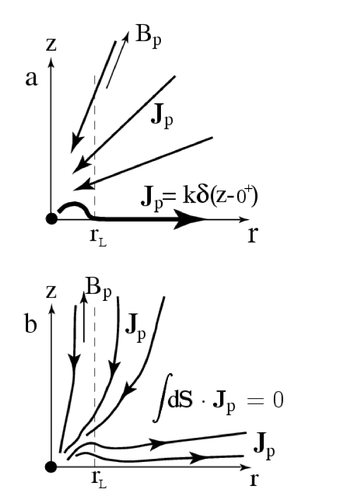
Figure 1: (a) Sketch of the poloidal current flow in a pulsar magnetosphere with a quasi-spherical wind with no jet as proposed by Contopoulos et al. (1999). (b) Sketch of the poloidal current flow with a collimated jet and a disk-wind. This solution is related to that proposed by Sulkanen and Lovelace (1990).

The poloidal current flow is sketched in Figure 1a. There is a corresponding positive current density $\propto\delta(z+0^{+})$ due to the lower half-space. Inside the light-cylinder the poloidal current sheet follows the dipole-like poloidal field lines to the star’s surface. This is required in order to have $H=0$ within the closed field line region of the magnetosphere. At the same time there is a delta-function toroidal current flow with

$$J_{\phi}=(c/4\pi)B_{r}(r,0^{+})\delta(z-0^{+})$$ (5)

for $r>1$. There is a corresponding positive toroidal current flow $\propto\delta(z+0^{+})$ due to the lower half-space. Inside the light-cylinder there is also a delta-function toroidal current sheet associated with the mentioned poloidal current sheet.

The magnetic field just above the equatorial plane for $r>1$ is ${\bf B}_{+}=B_{r}\hat{\bf{r}}+B_{\phi}\hat{{\hbox{\tenbg\char 30\relax}}~{}}$, and this is equal and opposite to the field just below the plane. The oppositely directed fields are unstable to annihilation. The electromagnetic stress $T_{zz}$ varies discontinuously from zero on the equatorial plane (by symmetry) to a finite value at $z=0^{+}$.

2.2.2 Jets

A second possibility is that there is a collimated jet along the $+z$ axis (and $-z$ axis) so that not all open field lines cross the light cylinder. The open field lines which do cross the light cylinder must obey equation (2). For the other open but collimated field lines ($0\leq r\leq r_{L}$,  $z\rightarrow\infty$), $H(\Psi)$ is arbitrary.

Thus $H(\Psi)$ is not determined for $\varphi\equiv\Psi/\Psi_{c}<1$. Because $H(0)=0$ we consider the simple dependence

$$H(\Psi)=k_{H}\left(\varphi-{1\over 2}\beta\varphi^{2}\right)~{},$$ (6)

where $k_{H}$ is an adjustable constant. As $k_{H}$ increases in equation (6) the axial current flow within the light-cylinder ($\propto dH/d\Psi$) increases. Owing to equation (2), $(HH^{\prime})_{c}$ is fixed at each step of the numerical iteration of $\Psi$. Of course, both $\Psi_{c}$ and $(HH^{\prime})_{c}$ evolve as the iteration proceeds. Consequently, we can calculate

$$\beta={1\over 2}\left[3-\left(1+{8\Psi_{c}(HH^{\prime})_{c}\over k_{H}^{2}}\right)^{1/2}\right]~{},$$

at each iteration.

We seek solutions without an equatorial current sheet. That is, we search for solutions with

$$\int_{0}^{\Psi_{eq}}d\Psi~{}{\cal F}=0~{}.$$ (7)

Figure 1b shows a sketch of the poloidal current flow.

3 Numerical Solutions

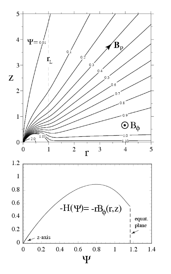
Figure 2: Quasi-spherical wind solution similar to that of Contopoulos et al. (1999). The jump in $H$ at $z=0$ is related the equatorial poloidal current current sheet shown in Figure 1a.

The numerical calculations of $\Psi$ for both cases of no jets and jets were done using successive iterations on a uniform $500\times 500$ mesh in a square region $r_{\rm max}\times z_{\rm max}=5\times 5$. We have obtained the same results for $600\times 600$ grid for a $6\times 6$ region. The initial $\Psi(r,z)$ used to start the iteration consists of the vacuum dipole field inside the light-cylinder and the straight line extrapolation of the field lines outside this cylinder. Convergence of the iterations is measured by the change of $\Psi$ between iterations. Figure 2 shows the solution $\Psi(r,z)$ and $H(\Psi)$ for the CKF case where there is no jet.

3.1 Solutions with Jets

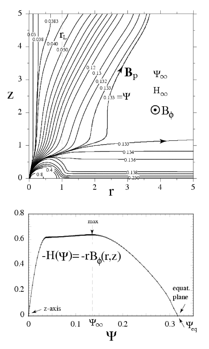
Figure 3: Pulsar magnetosphere with jet obtained by successive iteration of equation (1) with the constraint that $\int_{0}^{\Psi_{eq}}d\Psi{\cal F}=0$. $H(\Psi)$ within the light cylinder is given by equation (6) with $k_{H}=2.48$ and $\beta=0.9995$.

Figure 3 shows $\Psi(r,z)$ and $H(\Psi)$ for the case of a jet flow along the axis and a disk-wind in the equatorial plane where $k_{H}=2.48$. The flow has zero net poloidal current flow, $\int_{0}^{\Psi_{eq}}d\Psi{\cal F}=0$ and no current sheets. The main parameters of this solution are: along the $z-$axis $\Psi=0=H$; on the light-cylinder (at $z=5$) the values are $\Psi_{c}$ and $H_{c}=H(\Psi_{c})$; in the ${\bf B}_{p}=0$ region $\Psi_{\infty}$ and $H_{\infty}$; and on the equatorial plane $\Psi_{eq}$ and $H(\Psi_{eq})=0$. The numerical values are $\Psi_{c}=0.0384$, $H_{c}=0.6180$, $\Psi_{\infty}=0.133$, $H_{\infty}=0.637$, and $\Psi_{eq}=0.318$. This solution is not unique. For example, we have found an analogous solution for $k_{H}\sim 1$.

The total power output into both the upper and lower halfspaces is $\dot{E}_{\rm tot}=B_{0}^{2}r_{L}^{2}c\int_{0}^{\Psi_{eq}}d\Psi[-H(\Psi)]=0.152\dot{E}_{0}$, where $\dot{E}_{0}\equiv B_{0}^{2}r_{L}^{2}c$. In contrast, the total power output of the quasi-spherical wind solution is $\dot{E}_{tot}\approx B_{0}^{2}r_{L}^{2}c$ (e.g., McKinney 2006).

The jet flow consists of a region of collimated flux within the light-cylinder $r_{L}$ where $\Psi\leq\Psi_{c}=0.0384$, and a quasi-collimated region outside $r_{L}$ where $\Psi_{c}<\Psi<\Psi_{\infty}=0.133$. The power flow in the collimated jets is $\dot{E}_{\rm cjet}=\dot{E}_{0}\int_{0}^{\Psi_{c}}d\Psi[-H(\Psi)]=0.0155\dot{E}_{0}$. The power flow in the quasi-collimated flows is $\dot{E}_{\rm qcjet}=\dot{E}_{0}\int_{\Psi_{c}}^{\Psi_{\infty}}d\Psi[-H(\Psi)]=0.0595\dot{E}_{0}$. The power flow in the disk wind is $\dot{E}_{\rm dwind}=0.0767\dot{E}_{0}$. Thus, about $10\%$ of the total power goes into the collimated jet, $40\%$ into the quasi-collimated flow, and $50\%$ into the disk-wind.

3.1.1 Radial Force Balance of Jet

For conditions where a collimated jet exists, the $z-$derivatives in equation (1) vanish. The pulsar equation can then be written as

$${d\over dr}B_{z}^{2}+{1\over r^{2}}{d\over dr}\bigg{[}r^{2}\big{(}B_{\phi}^{2}-E_{r}^{2}\big{)}\bigg{]}=0~{},$$ (8)

which expresses the radial force balance. Multiplying this equation by $r^{2}dr$ and integrating from the axis to $r$ gives the radial virial equation

$$H^{2}=(r^{2}-1)\left({d\Psi\over dr}\right)^{2}+2\int_{0}^{r}{dr\over r}\left({d\Psi\over dr}\right)^{2}~{},$$ (9)

following Lovelace, Berk, and Contopoulos (1991).

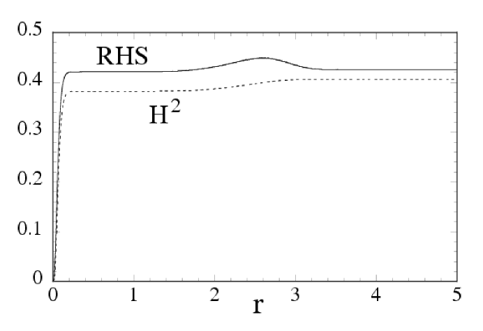
Figure 4: Two sides of equation (9) obtained from our numerical solution at $z=5$. RHS denotes the right-hand-side of the equation.

Figure 4 shows the two sides of equation (9) obtained from our numerical solution at $z=5$. There is a $\sim 10\%$ difference of the two sides of the equation. Calculations in a much larger region are required to determine whether or not the quasi-collimated flux outside the light-cylinder becomes collimated at very large distances.

3.1.2 Vertical Force Balance of Disk

The field solution shown in Figure 3 satisfies equation (1) accurately everywhere except close to the equatorial plane at $r^{2}\gg 1$. The reason for the discrepancy in this region can be understood by considering the vertical force balance for $z^{2}\ll r^{2}$ and $r^{2}\gg 1$ where $B_{z}^{2}\ll B_{r}^{2}$. For these conditions equation (1) is approximately

$$-r^{2}{\partial^{2}\Psi\over\partial z^{2}}=-{1\over 2}{dH^{2}\over d\Psi}=-{1\over 2}{\partial H^{2}\over\partial z}{1\over\partial\Psi/\partial z}~{}.$$

This can be rewritten as

$$-~{}{\partial\over\partial\xi}\left[-~{}{1\over 2}\left({\partial\Psi\over\partial\xi}\right)^{2}+~{}{1\over 2}H^{2}\right]=0~{},$$ (10)

where $\xi\equiv z/r$. This expresses the vertical force balance near the equatorial plane: The term $-(\partial\Psi/\partial\xi)^{2}$ represents the negative pressure of the electric field and it gives an upward force. The $H^{2}$ term is magnetic pressure due to the toroidal magnetic field and it exerts a downward force.

Figure 5 shows the vertical profiles of $\Psi$ and $H$. These profiles do not satisfy equation (10). The reason is that equation (1) omits the plasma kinetic energy density in all space including $z=0$ where the magnetic field reverses direction. Therefore we include the influence of the kinetic energy density as a term $K(\Psi)/2$ within the square brackets of equation (10). The origin of the kinetic energy is from the annihilation of the magnetic field. [A term of this form can be derived from the relativistic Grad-Shafranov (GS) equation of Lovelace et al. (1986). The right-hand side of equation (86) of this work includes a term $-4\pi\rho r^{2}dJ(\Psi)/d\Psi$, where $J=\gamma(1-rv_{\phi}/c)$ is the Bernoulli constant and $\gamma$ is the Lorentz factor. We may write $\rho r^{2}=f(\Psi)$ and $dK/d\Psi=8\pi f(\Psi)dJ(\Psi)/d\Psi$. The radial flow speed is $v_{r}=-cH^{-1}(\partial\Psi/\partial\xi)$ so that $\rho r^{2}v_{r}={\rm fct}(\Psi)$. ] Thus we obtain

$$\left({\partial\Psi\over\partial\xi}\right)^{2}=K(\xi)+H^{2}(\xi)-H_{\infty}^{2}~{},$$ (11)

where $H_{\infty}$ is the constant value of $H$ at large $\xi$. Clearly it is necessary to have $K+H^{2}\geq H_{\infty}^{2}$. Because $H(0)=0$ and $(\partial\Psi/\partial\xi)_{\xi=0}=0$, $K(0)=H_{\infty}^{2}$. Because $(\partial\Psi/\partial\xi)\rightarrow 0$ as $\xi$ increases, we have $K\rightarrow 0$ as $\xi$. A sufficient condition for having ${\bf E}^{2}<{\bf B}^{2}=B_{r}^{2}+B_{\phi}^{2}$ is $K<H_{\infty}^{2}$. To illustrate the behavior we consider the dependences $H^{2}=H_{\infty}^{2}[1-\exp(-\xi^{2}/\xi_{H}^{2})]$ and $K=H_{\infty}^{2}\exp(-\xi^{2}/\xi_{K}^{2})$ with $\delta\equiv\xi_{K}/\xi_{H}>1$.

Figure 6 shows the $\xi$ dependences of $\Psi$, $H$, and $rE_{z}$ calculated from equation (11) for an illustrative case which maintains the conditions of Figure 5 of $\Delta\Psi=\Psi_{eq}-\Psi_{\infty}=0.185$ and $H_{\infty}=0.638$. For this case we have taken $\delta=2$. As a result, $\xi_{K}=0.286$ which corresponds to a half-angle thickness of the disk of $\approx 16^{\circ}$. Near the equatorial plane the magnetic field has the form of an Archimedes’ spiral, namely, $dr/d\phi=-r_{L}(1-\delta^{-2})^{1/2}$. With this modification of the disk configuration, the global field solution involves no delta-function current sheets.

4 Conclusions

This work describes a new solution for the structure of the magnetosphere of an aligned rotator described by the force-free pulsar equation. This is obtained by adjusting the current flow along the poloidal field lines which remain within the light-cylinder. When this current flow is sufficiently large a collimated jet forms within the light-cylinder and a quasi-collimated flow forms outside of it. The solution is not unique. The jet is collimated by the toroidal magnetic field. At the same time an anti-collimated disk-wind forms in the vicinity of the equatorial plane. The anti-collimation is due to the toroidal magnetic field. The vertical force balance of the disk-wind requires the inclusion of a finite kinetic energy density near the equatorial plane. Roughly one-half of the open field lines go into the jets and the other half to the disk-wind. The total current flow in the jets is equal and opposite to the current flow in the disk. Thus there is no current sheet inside or outside of the light-cylinder.

Our jet/disk-wind solution represents an alternative to the quasi-spherical wind solutions where a major part of the current flow is in a current sheet. Such a current sheet is unstable to magnetic field annihilation. Furthermore, the way in which the configuration is reached is expected to be important. Consider a possible simulation experiment where the configuration is reached by dynamical evolution from an initially non-rotating star. The presence, distribution, and density of the initial plasma is important in that it is essential for the current flow as the star is spun up to a final rate. The value of the density of the background plasma was found to have an crucial role in determining the inflation magnetic loops threading a differentially rotating disk in relativistic particle-in-cell simulations (Lovelace, Gandhi, & Romanova 2005). The transition from one type of equilibrium to another remains to be investigated.

We thank A. Spitkovsky, M. Sulkanen, and A. Timokhin for valuable discussions. This work was supported in part by NASA grant NAG 5-13220 and NSF grant AST-0307817.

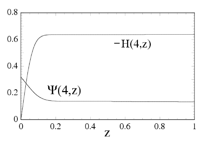
Figure 5: Vertical profiles of $\Psi$ and $H$ at $r=4$. At large $z$, $\Psi_{\infty}=0.133$ and $H_{\infty}=0.638$.

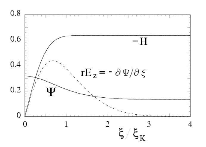
Figure 6: Vertical profiles of $\Psi$, $H$, and $rE_{z}$ calculated from equation (11) for illustrative conditions but maintaining $\Delta\Psi=\Psi_{eq}-\Psi_{\infty}=0.185$ and $H_{\infty}=0.638$.

References

- [1] Contopoulos, J., Kazanas, D., & Fendt, C. 1999, ApJ, 511, 351
- [2] Hester, J. J., Mori, K., Burrows, D., Gallagher, J. S., Graham, J. R., Halverson, M., Kader, A., Michel, F. C., & Scowen, P. 2002, ApJ, 577, L49
- [3] Komissarov, S.S.,& Lyubarsky, Y.E. 2004, Ap&SS, 293, 107
- [4] Komissarov, S.S. 2006, MNRAS, 367, 19
- [5] Komissarov, S.S., & Lyubarsky, Y.E. 2006, MNRAS, in press (astro-ph/0306162)
- [6] Lovelace, R.V.E., Mehanian, C., Mobarry, C.M., & Sulkanen, M.E. 1986, ApJ Supp., 62, 1
- [7] Lovelace, R.V.E., Berk, H.L., & Contopoulos, J. 1991, ApJ, 379, 696
- [8] Lovelace, R.V.E., Gandhi, P.R., & Romanova, M.M. 2005, Ap&SS, 298, 115
- [9] McKinney, J.C. 2006, MNRAS, in press (astro-ph/0601411)
- [10] Pavlov, G.G., Kargaltsev, O.Y., Sanwal, D., & Garmire, G.P. 2001, ApJ, 554, L189
- [11] Romanova, M.M., Chulsky, G.A., & Lovelace, R.V.E. 2005, ApJ, 630, 1020
- [12] Scharlemann, E.T., & Wagoner, R.V. 1973, ApJ 182, 951
- [13] Spitkovsky, A. 2004, in Camilo F., & Gaensler, B.M., eds, IAU Symposium No. 218, “Young Neutron Stars and Their Enviroments,” Astronomical Society of the Pacific, p. 357
- [14] Sulkanen, M.E., & Lovelace, R.V.E. 1990, ApJ, 350, 732
- [15] Timokhin, A.N. 2006, MNRAS, in press (astro-ph/0507054)
- [16] Ustyugova, G.V., Lovelace, R.V.E., Romanova, M.M., Li, H., and Colgate, S.A. 2000, ApJ, L21