Massive binaries in high-mass star-forming regions: A multi–epoch radial velocity survey of embedded O-stars

Abstract

We present the first multi-epoch radial velocity study of embedded young massive stars using near–infrared spectra obtained with ISAAC mounted at the ESO Very Large Telescope, with the aim to detect massive binaries. Our 16 targets are located in high–mass star–forming regions and many of them are associated to known ultracompact HII regions, whose young age ensures that dynamic evolution of the clusters did not influence the intrinsic binarity rate. We identify two stars with about 90 km/s velocity differences between two epochs proving the presence of close massive binaries. The fact that 2 out of the 16 observed stars are binary systems suggest that at least 20% of the young massive stars are formed in close multiple systems, but may also be consistent with most if not all young massive stars being binaries. In addition, we show that the radial velocity dispersion of the full sample is about 35 km/s, significantly larger than our estimated uncertainty (25 km/s). This finding is consistent with similar measurements of the young massive cluster 30 Dor which might have a high intrinsic binary rate. Furthermore, we argue that virial cluster masses derived from the radial velocity dispersion of young massive stars may intrinsically overestimate the cluster mass due to the presence of binaries.

1 Introduction

The formation and early evolution of young massive stars is not yet understood, motivating substantial observational and theoretical work. Observationally it is clear that most, or even all, massive stars form in clusters and OB–associations (de Wit et al., 2005). After their formation the massive stars remain hidden in their natal molecular cloud. This makes the youngest phases of massive stars difficult to study as only the infrared and the X–ray windows are accessible to detect the recently formed massive stars.

Only after a few million years, the massive stars become optically visible. By this time, many of them are found in multiple systems (Garmany et al., 1982; Zinnecker, 2003). In the Orion Trapezium cluster all but one of the massive stars are binaries with at least 1.5 companion per primary star on average (Preibisch et al., 1999).

A spectroscopic survey of the 30 Doradus cluster in the Large Magellanic Cloud suggests that most massive stars in that cluster are binaries. The radial velocity dispersion is much larger than what is estimated from the cluster dynamics and the dispersion is probably entirely dominated by binary orbital motions (Bosch et al., 2001). Numerical simulations show that the observations are consistent with the hypothesis that all (or most) stars in the cluster are binaries.

As those clusters are already a few million years old, dynamical cluster evolution might already have severely modified the binary fraction of the clusters members. In order to eliminate the influence of cluster dynamics on the binarity rate and to observe the initial binary fraction, other approaches have to be taken (Zinnecker, 2003).

Binarity studies of massive members of OB associations (e.g. Brown, 2001; Hillwig et al., 2006) can only provide a biased picture on the intrinsic binarity rate due to the evolution of massive stars over the typical lifetime ($\sim$ 5–20 Myr) of the associations.

For the determination of the binary rate of the most massive stars, the study of very young ($<$1 Myr) star–forming regions is necessary. Unfortunately, the multiplicity study of such young stars faces four serious observational difficulties: First, the large distances toward massive star–forming regions make direct imaging of close binaries very challenging and often impossible. Second, the youngest massive stars are deeply embedded and are only visible in the infrared regime. Third, these stars have very few and weak spectral lines in the infrared; in fact, they are often used as spectroscopic flat field sources. Fourth, being rapid rotators their spectral lines are broad and occasionally blending.

The recent years, however, proved that the line system in the K–band spectrum of massive stars, when observed with high enough signal–to–noise ratio and spectral resolution, still provides reliable spectral type classification (Hanson et al., 1996, 2005). The K–band spectral atlas has been applied by Bik et al. (2005) to 40 high-mass stars in high–mass star-forming regions, mostly close to ultracompact H II regions using the ISAAC/VLT infrared instrument. To demonstrate the K–band spectra of young OB stars we show some representative spectra from this survey in Fig. 1. The Bik et al. (2005) survey yields a unique spectroscopic data set on the youngest observable massive stars.

Aiming to determine the intrinsic multiplicity of the massive stars we obtained second– and occasionally third–epoch spectra for 16 targets of this sample using an identical instrument setup. By identifying the variability of the massive stars’ radial velocities we probed the presence of close, massive companions and identified at least two embedded, close, and massive multiple systems.

Figure 1: Representative VLT/ISAAC K–band spectra of OB stars: the CIV line is at 2.078 $\mu$m, the He I line is at 2.113, the NIII line is at 2.116 $\mu$m, the HI is at 2.166, the HeII is at 2.189 $\mu$m.

2 Observations and data reduction

Our target list consists of spectroscopically confirmed massive stars identified via near–infrared photometry. Kaper et al. (2006) carried out multi–color NTT/SOFI imaging of 44 IRAS sources with colors typical to ultracompact HII regions and identified young massive star candidates via their position on the color-magnitude diagram (red and bright). In 31 of these regions Bik et al. (2005) carried out near–infrared spectroscopy confirming 38 massive stars.

This survey provided spectral type classification of the massive stars and served as the first-epoch radial velocity measurement for our survey. By re-observing the most massive stars (O and early B) we extended these measurements into a multi–epoch radial velocity survey. In order to maximize the homogeneity of the data at different epochs we used the same slit positions for all but three objects. In these three cases only one massive star was covered in the original slit position: the new slit orientation allowed probing additional bright stars in the regions. For five stars we were able to obtain an additional, third–epoch measurement.

Following the nomenclature adopted in Kaper et al. (2006) and Bik et al. (2005) we will name the objects after the first 5 digits (i.e. the right ascension) of the IRAS point source they are associated with, followed by a running number from our initial photometric identification (e.g. object 324 in IRAS 10049-5657 we refer to as 10049nr324).

2.1 ISAAC Observations

The spectroscopic data presented in this paper were obtained during several runs between March 2000 and June 2002 using the 1024$\times$1024 pixel ISAAC near–infrared camera and spectrograph (Moorwood, 1997) mounted at the Nasmyth focus of the UT1 of the Very Large Telescope of the European Southern Observatory at Cerro Paranal, Chile. Table 1 lists the targets and the journal of observations

Table 1: Journal of observations and the target list.

IRAS Source	Slit ID	1st Epoch	2nd Epoch	3rd Epoch
IRAS 10049-5657 (catalog )	Single	00/03/19	02/06/19	2 $\times$ 02/06/20
IRAS 15408-5356 (catalog )	Single	00/03/20	02/06/19	02/06/20
IRAS 16177-5018 (catalog )	Slit 1	00/05/08	02/06/19	02/06/20
IRAS 16177-5018 (catalog )	Slit 2	00/05/08	02/06/19	02/06/20
IRAS 16571-4029 (catalog )	Single	00/05/08	02/06/20	—
IRAS 17149-3916 (catalog )	Single	00/05/19	02/06/19	—
IRAS 17258-3637 (catalog )	Single	00/05/19	02/06/19	—
IRAS 18449-0158 (catalog )	Slit 1	00/06/20	02/06/19	02/06/20
IRAS 18507+0110 (catalog )	Slit 1	00/07/12	02/06/19	—
IRAS 18507+0110 (catalog )	Slit 2	00/06/20	02/06/19	—

The observations were carried out in a standardized fashion to ensure the homogeneity of the data set. For all objects the observed spectral range extends from 2.075 $\mu$m to 2.2 $\mu$m, centered on 2.134 $\mu$m with three exceptions: During the first epoch observations the objects IRAS 10049-5657 and IRAS 15408-5356 have been observed with a spectral range centered at 2.129 $\mu$m, while in the second epoch the object 10049-5657 has been observed additionally with a spectral range centered at 2.138 $\mu$m to also cover the He II line at 2.185 $\mu$m. In order to reach the highest spectral resolution we used the smallest available slit width of 0.3″. The effective resolution with a resolving power of R $\simeq$ 10,000 corresponds to a radial velocity resolution of $\simeq$ 30 km/s.

In order to free the spectra from Earth’s atmospheric influence, after each science target, we observed a telluric standard with an identical airmass. As telluric standards we used A–type stars, which display no lines apart from the Br$\gamma$ line in the spectral regime in question. After every standard star observation a flat field has been obtained in order to correct for fringing patterns which become visible in high S/N K-band spectra.

2.2 Data Reduction

The spectra from the first and the second epoch are reduced in an identical way in order to obtain more homogeneous measurements. A detailed description of the reduction process is given in Bik et al. (2005) and in Apai (2004) and is performed using standard IRAF and IDL routines. In the following we will only briefly overview the non-standard and critical reduction steps, such as the wavelength calibration and the telluric line removal.

The pixel–to–wavelength calibration is performed using the OH emission line spectrum present in the observed spectra (Rousselot et al., 2000) with the IRAF task identify. The derived wavelength solution was typically better than 0.2 pixel (3 km s^-1). This wavelength solution was then step-by-step shifted and matched in the spatial direction along the slit. An independent wavelength calibration has been derived for each night.

The telluric standard stars, observed at matching airmasses (with typical differences less than 0.1), are used to remove the telluric absorption lines in the spectra. We applied main sequence A–type stars as telluric standards because their K–band spectra are featureless except for the Br$\gamma$ line. The Br$\gamma$ line was removed in two steps: First, the telluric features are removed from the $K$–band spectrum of the telluric standard using a high–resolution telluric spectrum (obtained at NSO/Kitt Peak). This spectrum is taken under very different sky conditions, so numerous spectral remnants remain visible in the corrected standard star spectrum. Without this “first-order” telluric–line correction, however, a proper fit of Br$\gamma$ cannot be obtained. In the second step the Br$\gamma$ line was fitted by a combination of two exponential functions. The error on the resulting Br$\gamma$ equivalent width of our target star was about 5 %. After the removal of the Br$\gamma$ line of the A star, the telluric lines are removed using the IRAF task telluric. The task applies a cross-correlation procedure to determine the optimal shift in wavelength and the scaling factor in line strength, which could be adjusted interactively. The shifts were usually a few tenths of a pixel; also the scaling factors are modest ($\sim 10$ %).

3 Radial Velocity Measurements

The final step of the procedure was the measurement of the radial velocity of each object at a given epoch. As our science goal is the detection of close binaries, we were focusing on deriving relative radial velocities and did not aim at deriving the absolute values. For the sake of simplicity, we always chose the first epoch observation (see, Tab. 1) as the radial velocity zero point and compared the subsequent epoch(s) to this reference value by using the IRAF package RV and the fxcor task.

This package is widely applied for accurately measuring the radial velocities by means of cross-correlation. As the package has been discussed by Fitzpatrick (1994) and Rodes et al. (1998), we only summarize here a few essential points and non-standard choices of parameters.

The radial velocity is determined by cross-correlating the first epoch measurement to the later epoch ones, after correcting for any differences in heliocentric velocities. However, only the photospheric lines of the massive stars carry valuable information on the radial velocity. The continuum is usually dominated by telluric line remnants and might influence the cross-correlation. Therefore, the individual spectral regions of interest have been selected manually after the inspection of each reduced spectrum. In practice, the He I and Br$\gamma$ lines are mostly used for the cross-correlation (see, Appendix A for details per object).

The actual radial velocity difference ($\Delta$RV), i.e. the wavelength shift between the two spectra is derived from the cross-correlation function: Its maximum is where the shifted second epoch spectrum matches best the first epoch one. The maximum of the correlation function was identified by fitting a Gaussian function on the peak. To adopt our measurement to the rather broad lines of the massive stars we enlarged the default short fitting interval to a maximum of 100 pixel interval. Fig. 2 shows an example for the radial velocity determination and the fitting of the cross-correlation function.

Figure 2: Example for the cross–correlation based relative radial velocity determination. The upper panel shows the object spectrum and the horizontal bars mark the wavelength range which was used for the cross-correlation. The middle panel shows the complete cross-correlation function, while the lower one displays a magnified region around the peak. The dashed curve is the fitted Gaussian and the horizontal solid line is its full width at half maximum. This plot is the output of the IRAF script fxcor.

3.1 Error Analysis

The observations described in this paper represent a pilot effort to derive radial velocity variations for deeply embedded massive stars. These measurements are complex making a detailed error analysis essential. In the following we discuss the impact of the individual error sources and measure the total error from quasi-simultaneous observations.

3.1.1 Telluric Line Residuals

All our spectra bear to some extent the imprint of Earth’s atmosphere in the form of fixed–wavelength telluric lines. Although the individual line residuals have modest strength, their integrated power could bias the $\Delta$RV measurements towards the zero values.

In order to test this possibility, we repeated the radial velocity measurements but used a photospheric–line–free, pure continuum spectral region between 2.125 – 2.1500 $\mu$m for the cross-correlation. This region is dominated by low–level telluric line residuals. If the cross–correlation would be influenced by the presence of the residuals of the given telluric lines, the radial velocity difference would give a systematic signal close to $\Delta$RV=0. In contrast, the cross–correlation returns randomly distributed values between $\sim$ 1100 and -1100 km/s indicating that the telluric line residuals do not introduce any systematic high-power signal to the cross–correlation function and therefore have a negligible influence on the real, high–power correlation functions of the stellar photospheric lines.

3.1.2 Nebular Line Contamination

Br$\gamma$ and He I emission lines are often present in the nebula surrounding young massive stars and may bias simple RV–determination. The analysis of the nebular spectra close to our sources has demonstrated that these lines are unresolved at our resolution. The He I line’s typical intensity in the nebular spectra is only $\sim$1% of that of the line in the stellar spectra and thus has only a negligible effect on our RV–determination. In order to ensure that the more intense Br$\gamma$ does not bias our RV–determination, we excluded the Br$\gamma$ line center from the cross–correlation of our stellar spectra thereby relying only on the non–contaminated wings of the Br$\gamma$ line.

3.1.3 Wavelength Calibration

We derived a wavelength calibration for each night of the observations. The error of the wavelength solution is well characterized by the comparison to the OH-line catalogue containing thousands of narrow spectral lines. The wavelength calibration was typically better than 0.2 pixel, corresponding to a RV inaccuracy of 3.4 km/s for unresolved lines.

3.1.4 Peak Fitting Methods and their Errors

The $\Delta$RV is determined by maximizing the cross–correlation function of the spectra from different epochs (see also Sect. 3). Localizing the maximum is accomplished by fitting the peak of the cross–correlation function. We tested different peak–fitting methods, including Gaussian, parabolic, and Lorentzian fits, as well as IRAF’s Center1D routine. All algorithms but the Center1D provide formal error estimates for the fit results. In the next section we discuss the results of the different fitting methods.

For our data set we found that the Gaussian, Center1D, and Lorentzian methods gave statistically very similar results. Although the parabolic approximation led to consistent results for most of the objects, in some cases it provided an unstable, out–of–bounds solution.

Throughout the paper we used the Gaussian fitting, as this provided the most robust results. The fitted regime was 100 pixels corresponding to about 1700 km/s velocity difference ensuring that also the wings of the cross–correlation peak are included.

3.1.5 Quasi–Simultaneous Observations

For four objects we obtained subsequent spectra in two slit positions with typical time differences of $\sim$1 hr. Assuming that the RVs did not change significantly between the two observations, these quasi–simultaneous observations give a good impression of the accuracy with which we are able to measure radial velocity differences.

Using these pairs of observations we tested the consistency of the different RV determination methods (see, Table 2). In our test we used direct comparison (cross–correlation of two spectra) and indirect comparison (comparison of the deviations from a fiducial zero point, i.e. the first epoch RV). We also varied the function fitted to determine the peak of the cross–correlation functions in combination with the direct and indirect comparisons.

Assuming that the radial velocity of our four stars does not change on timescales of an hour, all measured RV differences should be zero (see, Table 2). The higher values seen here arise from two effects: the error of the RV determination and the possibility of RV variations due to stellar multiplicity. If the RV changes are negligible (i.e. none of the four stars are close binaries), the observed differences are characteristic for the measurement error; otherwise they overestimate the errors. Lacking the knowledge on the multiplicity of these four stars the RV differences derived in the following should be taken as upper limits for the measurement errors.

The means of the absolute differences for the different fitting methods are listed in Table 2. The direct method has the smallest error (19 km s^-1), while among the indirect comparisons the Gaussian method (24.2 km s^-1) is the most accurate and robust. By understanding the differences between the direct and indirect methods we can estimate the error budget from the different comparison steps: The direct comparison of two quasi-simultaneous spectra contains the statistical errors on 2 measurements and the error of 1 cross-correlation and peak fitting. The indirect Gaussian method is carrying the errors from 3 measurements, 1 calibration difference and 2 correlations.

Our results as presented in Sect. 4 use the first epoch spectra as reference for the later observations and therefore contain the errors from 2 measurements, 1 calibration difference and 2 correlations. Their total error is in between the errors of the quasi-simultaneous direct and indirect Gaussian methods described above. Thus, the total error on our RV-difference measurements is between 19.0 km/s and 24.2 km/s, somewhat higher than the 14.7 km/s mean of the formal error estimates of the IRAF routine fxcor.

Table 2: Radial Velocity differences of the four quasi-simultaneous observations as measured by different methods. The first column is the identification of the observations as given in Table 1, the second column gives the epoch when the quasi–simultaneous observations were obtained, the third column gives the RV difference derived from fitting a Gaussian function on the peak of the cross-correlation function of the two spectra. The other columns are the RV differences obtained by first correlating each second and third epoch spectra to the first epoch one and making the difference of the RV shifts. The last three columns differ in the function used for finding the peak of the cross-correlation function.

Object	Epoch	Direct Gaussian	Gaussian	Center 1D	Lorentz
		[km s-1]	[km s-1]	[km s-1]	[km s-1]
10049nr324	3	–18.0	–18.0	–11.2	–15.7
10049nr411	3	–4.6	39.9	56.9	40.0
16177nr1020	2	15.2	3.8	–18.8	–7.1
18507nr373	2	38.1	35.1	—	39.4
Mean of	Absolute Differences	19.0	24.2	29.0	25.0

4 Results

The main results of our multi-epoch spectroscopic campaign are summarized in Table 3. This table provides a compilation of the measured radial velocity variations, the spectral types as derived by Bik et al. (2005), as well as the epochs used for the cross–correlation. We will first show the results on 2 individual objects where we have detected a large velocity difference. After that the distribution of the radial velocities is presented.

Table 3: Results of the RV cross–correlation. The columns list the IRAS source, the target ID, spectral type, night of the second epoch, radial velocity change relative to the first epoch measurements and their formal errors.

IRAS source	Star	Sp. Type	Epochs	$\Delta$ RV [km/s]
IRAS 10049-5657	10049nr324	O3V – O6.5V	1,3	14 $\pm$ 11
	10049nr324	O3V – O6.5V	1,3	32 $\pm$ 12
	10049nr324	O3V – O6.5V	1,2	15 $\pm$ 14
	10049nr411	O3V – O4V	1,3	27 $\pm$ 14
	10049nr411	O4V – O4V	1,3	-13 $\pm$ 29
	10049nr411	O3V – O4V	1,2	87 $\pm$ 5
IRAS 15408-5356	15408nr1410	O5V – O6.5V	1,2	13 $\pm$ 20
	15408nr1410	O5V – O6.5V	1,3	27 $\pm$ 17
	15408nr1454	O8V – B2.5V	1,2	21 $\pm$ 14
	15408nr1454	O8V – B2.5V	1,3	18 $\pm$ 25
IRAS 16177-5018	16177nr1020	O5V – O6.5V	1,3	-13 $\pm$ 9
	16177nr1020	O5V – O6.5V	1,2	-19 $\pm$ 14
	16177nr1020	O5V – O6.5V	1,2	-16 $\pm$ 16
	16177nr271	O8V – B2.5V	1,3	33 $\pm$ 10
	16177nr271	O8V – B2.5V	1,2	16 $\pm$ 8
	16177nr405	O5V – O6.5V	1,2	-2 $\pm$ 11
IRAS 16571-4029	16571nr820	O8V – B1V	1,3	32 $\pm$ 6
IRAS 17149-3916	17149nr895	O5V – O6.5V	1,2	1 $\pm$ 10
IRAS 17258-3637	17258nr1558	O8V – B2.5V	1,3	6 $\pm$ 8
	17258nr378	O8V – B1V	1,3	-95 $\pm$ 12
IRAS 18006-2422	18006nr770	O8V – B1V	1,3	-13 $\pm$ 15
IRAS 18449-0158	18449nr319	O5V – O6V	1,2	-29 $\pm$ 24
	18449nr319	O5V – O6V	1,3	-30 $\pm$ 24
IRAS 18507+0110	18507nr262	O5V – O8V	1,2	-35 $\pm$ 14
	18507nr373	B1V – B2.5V	1,2	-24 $\pm$ 24
	18507nr373	B1V – B2.5V	1,2	-59 $\pm$ 18
	18507nr389	O8V – B2.5V	1,2	-2 $\pm$ 10

4.1 Two compact massive binaries

Two stars, 17258nr378 and 10049nr411, show radial velocity variations as large as $\sim$90 km/s between the two measurements. Variations of such a large amplitude can be most plausibly explained by the assumption that these stars are close massive binaries.

The orbital parameters of these two systems cannot be derived from the only two epoch measurements available, but the amplitude of the RV–change suggests close, massive companions. For example, considering the case of 17258nr378 with a primary mass of $\sim$ 15 M_⊙ and assuming a circular orbit with an inclination of 70$\arcdeg$, the observations are consistent with a secondary of mass 9.5 M_⊙ and orbital radius less than $\sim$0.4 AU. Star 10049nr411 is a much more massive star (M=40–60 M_⊙) and the observed large $\Delta$RV requires a companion even more massive or on a shorter–period orbit than the secondary in 17258nr378. As an example, a 50 and 20 M_⊙ binary at a separation of 0.5 AU and an inclination of 70$\arcdeg$ would be consistent with the measured radial velocity variation.

The observations of these two sources demonstrate that at least 20% of the young massive stars are in compact binary systems with massive secondaries. We discuss the implications of this finding in Sect. 5.

4.2 A population of young, massive binaries?

The distribution of the RV-differences is shown in the histogram in Fig. 3. The mean value of the 27-point sample is 0 km/s and the standard deviation is 34.5 km/s. This is significantly larger than the mean error which we estimated to be between 19 and 24 km/s (see, Sect. 3.1.5).

If the two binary stars identified above, 17258nr378 and 10049nr411, are removed from the sample the standard deviation of the remaining measurements is 24 km/s, marginally consistent with our most pessimistic error estimates.

Although the RV-distribution is likely broader than the expected distribution of single stars, the limited number of sources that could be observed in our survey does not allow to detect a statistically significant difference from a single star population observed with our radial velocity accuracy.

Future infrared surveys using higher resolution instruments – such as VLT/CRIRES with a resolution of 100,000 corresponding to 3 km/s — will be able to reliably discriminate between the population of single and binary stars and place constraints on the fundamental properties of the typical compact binaries, such as mass and semi–major axis.

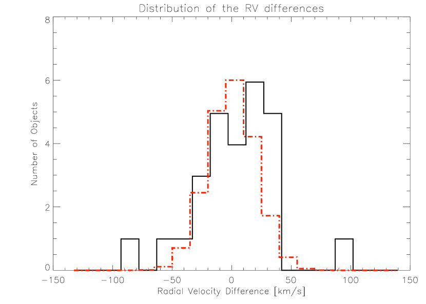
Figure 3: Histogram of the observed radial velocity differences of the systems at different epochs plotted with the solid black line. The two outliers are very good candidates for being close binary stars. The dot–dashed line indicates a hypothetic distribution of a single star population observed with a normally distributed measurement error 20 km/s.

5 Discussion

In the previous section we have shown that we have identified two compact massive binary systems. Additionally, the distribution of the radial velocity measurements is larger than the error on the measurements. This might reflect the identification of a massive binary population. In this section we compare our results with other radial velocity studies and discuss the possible implications of our findings.

5.1 Previous binarity studies of massive stars

Our survey probes the multiplicity of massive stars at the youngest ages and complements well existing surveys which mainly focused on optically visible and thus somewhat older massive stars.

The best–studied massive stars are arguably the members of the Trapezium system. These massive stars in the $\sim$ 1 Myr–old Orion Nebula Cluster have at least 1.5 companions per primary star on average, as shown by bispectrum speckle interferometry (Preibisch et al., 1999). However, it is yet unclear, how well this binary rate represents the intrinsic binarity of these massive stars and whether or not cluster dynamics have already changed the structure of the Orion Nebula Cluster (see, e.g. Hillenbrand & Hartmann 1998; Bonnell & Davies 1998).

An ideal target for measuring the binarity rate for a large number of young massive stars in an identical environment is the massive stellar cluster R136, which ionizes the Large Magellanic Cloud starburst cluster 30 Doradus. This cluster shows three distinct peaks in its star formation history at 5 Myrs ago, 2.5 Myr and $<$1.5 Myr ago (Selman et al., 1999). The spectroscopic survey of Bosch et al. (2001) presented reliable RVs for 55 stars in the 30 Dor and found a RV dispersion of $\sim$ 35 km/s. This dispersion is much larger than what is estimated from the cluster dynamics and the dispersion is probably entirely dominated by binary orbital motions. Numerical simulations show that the observations are consistent with the hypothesis that all stars in the cluster are binaries.

Although this work provides a strong argument for the intrinsically high binary rate, the 30 Dor cluster is unlikely to be representative for the galactic massive star–forming environments due its violent starburst nature and the multiply–peaked star formation history. Additionally, because of the multiply–peaked star formation process in this cluster, the dynamically formed binaries may contaminate the intrinsic binarity rate to an unknown extent.

This latter velocity dispersion is virtually identical to the dispersion we find in our multi–epoch, multi–cluster survey. Although a larger sample is required to firmly separate the contributions from the measurement uncertainties and the multiple systems, our result suggests that the velocity dispersion is the same or smaller for even younger systems and supports the interpretation by (Bosch et al., 2001) of close binary systems as the origin of the radial velocity dispersion.

Detecting double–line spectroscopic binaries (SB2) requires identifying the two line systems arising from the two stellar components only possible with a spectral resolution high enough compared to the average separation and width of the lines. The very few and very broad lines of massive stars makes such detections considerably more difficult than the detection of single–line (SB1) binaries. Due to the modest spectral resolution (R$\sim$10,000) and limited contrast our study is thus largely insensitive to double–line spectroscopic binaries (SB2) and could detect only single–line (SB1) binaries. However, optical spectroscopic studies of more evolved OB–stars suggest that the frequency of SB1 binaries are similar or comparable to that of SB2 (e.g. Mason et al. 1998). Thus, the complete binary fraction of the target sample is likely exceeding the lower limit established through the current survey.

5.2 The effect of massive binaries on cluster virial mass estimates

The large variations of the RVs of the young massive stars in our sample demonstrate the effect of massive binaries on the cluster’s RV dispersion. We showed that excluding the known binary systems decreases the RV dispersion from 35 km/s to 24 km/s and possibly even more, demonstrating that in a random sample of $\sim$20 young stars at least 1/3 of the RV dispersion is caused by binaries.

The RV dispersion of unresolved extragalactic clusters is a frequently used tool to derive virial mass estimates (e.g. $M\approx\Delta RV^{2}$). The light of massive clusters is dominated by its most massive members. We point out, that masses derived under the assumption that these young massive clusters are virialized will overestimate the masses, in some cases to a significant extent. Should our targets be in an unresolved cluster, the cluster mass would have been overestimated by 2.3 times.

Note, however, that if the binarity of massive stars is independent of the cluster mass in which they formed, this effect will be less important for very massive clusters ($>$100 OB–stars), where the cluster radial velocity dispersion will dominate over the close binaries’ velocity dispersion.

5.3 Formation scenarios for massive stars

Massive star formation still poses a significant observational and theoretical challenges, but evidence is mounting for the disk–accretion scenario for stars up to 30 M_⊙ (Beuther et al., 2006). It is yet unclear, whether this mechanism extends to the highest stellar masses and whether or not the stellar coalescence plays role in the formation of massive stars (Bonnell et al., 1998; Bonnell & Bate, 2005).

When discussing the difficulty of observationally testing these scenarios, Bally (2002) points out the intrinsic multiplicity ratio as a potentially strong constraint. He notes that a high frequency of nearly-equal mass massive binaries should form in the clusters where stellar collisions are occurring (Bonnell, 2002).

Our survey demonstrates that at least 20% and probably an even larger fraction of the massive stars form in compact, massive multiple systems. Comparison to the Monte Carlo simulations by Bosch & Meza (2001) adopted to our observations, which take into account the observational biases and stellar parameter distributions, suggest that our observations are consistent with most if not all our targets being compact, massive binaries (Bosch, priv. comm.).

This finding may lend further support to the coalescence scenario, but may also be consistent with the disk accretion model, whose implications on intrinsic binarity have not yet been explored. The significant fraction of binary stars for stellar mass ranging from brown dwarfs (Burgasser et al., 2006) through T Tauri stars (Duchene et al., 2006) to massive stars suggests that binarity is a fundamental ingredient of star formation.

6 Conclusions

We present the first multi-epoch spectroscopic radial velocity survey of massive stars associated to young (ultra–)compact H II regions. The radial velocity variations indicate massive companions in at least two of our 16 targets. The broad $\Delta$RV-distribution of our sample resembles the distribution found by the single–epoch optical spectroscopy of the starburst cluster R 136 (Bosch et al., 2001). The main results of this work are:

– We identify an O5/O6 and an O9/B1 spectral type star displaying RV-variations as large as $\sim$90 km/s and we show that they are close massive binary stars.

– Our survey demonstrates that at least 20% of the O–stars in ultracompact HII regions are in close, massive multiple systems, and may be consist with most if not all systems being compact binaries.

– The observed $\Delta$RV distribution of the observed sample is 35 km/s, inconsistent with single-star population. The distribution of the sub-sample excluding the two identified massive binaries is 25 km/s, still broader than (but marginally consistent with) the distribution of single star population observed with our RV–accuracy.

– We point out, that the presence of compact massive binaries on the overall RV–dispersion will bias virial mass estimates of stellar clusters towards higher masses.

– High–resolution, sensitive near-infrared spectroscopy is a powerful tool to study the intrinsic properties of massive stars. Our RV accuracy limit is set by the combination of the spectral resolution and the uncertainties in telluric line correction. Future studies capable of reaching $\sim$15 km/s or better accuracy on a similar or larger set of targets will be able to place statistical constraints on the intrinsic frequency of compact, massive binary stars.

Appendix A Discussion of individual objects

In the following we list the comments on the individual objects; a more detailed description and figures of the individual spectra are shown in Apai (2004).

IRAS 10049$-$5657: Star #324 is identified as O3V—O6.5V spectral type (Fig. 1). He I absorption at 2.11 $\mu$m is visible in the spectrum setting an upper limit of O5V—O6.5V to the spectral type. However the absence of C IV suggests an O3—O4V spectral type (see Bik et al., 2005). The telluric line removal was efficient but the Br$\gamma$ line is over-subtracted due to overlapping nebular emission from the other dithering position. As its peak was unreliable, we included only the wings of the Br$\gamma$ line in our cross-correlation.

Star #411 is of earlier spectral type (O3V—O4V) as no He I line is detected and has weaker spectral lines. Although the telluric subtraction is in general good, the Br$\gamma$ line is contaminated by some telluric residuals and suffers nebular line over-subtraction. The N III line is broad and not well–defined. However, cross-correlations of the wings of Br$\gamma$ and the N III line gives very similar results to that from the correlation of only the N III line, proving the reliability of the fit. The third epoch measurement gives a relative shift as large as $\sim$88 km/s.

IRAS 15408$-$5356: Star # 1410 is an early–type star with an estimated spectral type of O5V—O6.5V. Although some fringing and telluric lines are present, the cross-correlation function has a sharp maximum. Star # 1454 is an O8V—B2.5V spectral type star with the HeI line in absorption. The equivalent width of the Br$\gamma$ line is very close to the division line between the O8V—B1V and B1V—B2.5V spectral classes (see Bik et al., 2005, for more details). The telluric correction is good, but the Br$\gamma$ line has some nebular line over–subtraction. We used the He I line as well as the wings of the Br$\gamma$ line for the cross-correlation.

IRAS 16177$-$5018: Star # 271 has a spectral type of O8V—B2.5V with weak HeI and Br$\gamma$ absorption. The wings of the Br$\gamma$ line are useful for the cross–correlation. The 2nd epoch observations is of somewhat worse quality than the 3rd epoch. Star #405 is an early-type star with O5V—O65.V classification. The lack of absorption lines and the weakness of the emission lines makes the radial velocity measurement difficult. Another very early-type star is # 1020, which is classified as of O5V—O6.5V spectral type. The Br$\gamma$ line in its spectrum is filled in by nebular line emission and was completely excluded from the fit.

IRAS 16571$-$4029: Star # 820 is of spectral type O8V–B1V. Although the spectra suffer from rather stronger telluric line residuals, the Br$\gamma$ and He I line are however not affected. The double-peaked He I line provides a firm basis for the cross-correlation.

IRAS 17149$-$3916: Star # 895 has been classified as of O5V—O6.5V spectral type. The C IV, N III and the Br$\gamma$ line are present.

IRAS 17258$-$3637: Object # 1558 is an O8V—B2.5V spectral type star. The spectra suffer from telluric residuals; in the second epoch Br$\gamma$ is contaminated by nebular emission. Star # 378 is classified as O8V—B1V spectral type. Although the telluric line removal is not good, the atmospheric lines are free from residuals. The spectra from the two epochs are obviously shifted, while the telluric lines coincide. This star is a strong candidate for being a binary star.

IRAS 18006$-$2422: Star # 770 is an O8V—B1V type star. The spectra are of good quality apart from some telluric residuals.

IRAS 18449$-$0158: Star # 319 is an early type with an O5V—O6V classification. The Br$\gamma$ line has a strange shape, might be affected by telluric residuals. Still, the N III and He I line give strong basis for the fit. In the third epoch spectrum the Br$\gamma$ line looks normal, but the overall telluric residuals are slightly worse.

IRAS 18507$+$0110: The spectra of star # 262 shows some fringes, but the telluric removal was successful. The spectral classification of this star is O5I—O8I, and it is likely not a main sequence star but possibly a super–giant or possesses an unusually strong stellar wind. The star # 373 has been observed two times with two different slit orientations the night of 19th June 2002. This B1V—B2.5V spectral type star provides a relatively weak cross–correlation peak due to the improper telluric line removal. The second slit orientation on this IRAS source included the O8V—B2.5V star # 389. Its spectrum shows characteristic He I absorption lines, which give a firm basis for multi-epoch cross-correlation.

Facilities: VLT (ISAAC).

References

- Apai (2004) Apai, D. 2004, Ph.D. Thesis, University of Heidelberg
- Bally (2002) Bally, J. 2002, in ASP Conf. Ser. 267: Hot Star Workshop III: The Earliest Phases of Massive Star Birth, 219
- Beuther et al. (2006) Beuther, H., Churchwell, E. B., McKee, C. F., & Tan, J. C. 2006, ArXiv Astrophysics e-prints
- Bik et al. (2005) Bik, A., Kaper, L., Hanson, M. M., & Smits, M. 2005, A&A, 440, 121
- Bonnell (2002) Bonnell, I. A. 2002, in ASP Conf. Ser. 267: Hot Star Workshop III: The Earliest Phases of Massive Star Birth, 193
- Bonnell & Bate (2005) Bonnell, I. A. & Bate, M. R. 2005, MNRAS, 362, 915
- Bonnell et al. (1998) Bonnell, I. A., Bate, M. R., & Zinnecker, H. 1998, MNRAS, 298, 93
- Bonnell & Davies (1998) Bonnell, I. A. & Davies, M. B. 1998, MNRAS, 295, 691
- Bosch & Meza (2001) Bosch, G. & Meza, A. 2001, in Revista Mexicana de Astronomia y Astrofisica Conference Series, ed. A. Aguilar & A. Carramiñana, 29
- Bosch et al. (2001) Bosch, G., Selman, F., Melnick, J., & Terlevich, R. 2001, A&A, 380, 137
- Brown (2001) Brown, A. 2001, Astronomische Nachrichten, 322, 43
- Burgasser et al. (2006) Burgasser, A. J., Reid, I. N., Siegler, N., et al. 2006, ArXiv Astrophysics e-prints
- de Wit et al. (2005) de Wit, W. J., Testi, L., Palla, F., & Zinnecker, H. 2005, A&A, 437, 247
- Duchene et al. (2006) Duchene, G., Delgado-Donate, E., Haisch, Jr., K., Loinard, L., & Rodriguez, L. 2006, ArXiv Astrophysics e-prints
- Fitzpatrick (1994) Fitzpatrick, M. 1994, in ASP Conf. Ser. 61: Astronomical Data Analysis Software and Systems III, 79
- Garmany et al. (1982) Garmany, C. D., Conti, P. S., & Chiosi, C. 1982, ApJ, 263, 777
- Hanson et al. (1996) Hanson, M. M., Conti, P. S., & Rieke, M. J. 1996, ApJS, 107, 281
- Hanson et al. (2005) Hanson, M. M., Kudritzki, R.-P., Kenworthy, M. A., Puls, J., & Tokunaga, A. T. 2005, ApJS, 161, 154
- Hillenbrand & Hartmann (1998) Hillenbrand, L. A. & Hartmann, L. W. 1998, ApJ, 492, 540
- Hillwig et al. (2006) Hillwig, T. C., Gies, D. R., Bagnuolo, Jr., W. G., et al. 2006, ApJ, 639, 1069
- Kaper et al. (2006) Kaper, L., Bik, A., Comerón, F., & Hanson, M. M. 2006, to be sumbitted to A&A.
- Mason et al. (1998) Mason, B. D., Gies, D. R., Hartkopf, W. I., et al. 1998, AJ, 115, 821
- Moorwood (1997) Moorwood, A. F. 1997, in Proc. SPIE Vol. 2871, Optical Telescopes of Today and Tomorrow; Ed.: Ardeberg, A. L., 1146–1151
- Preibisch et al. (1999) Preibisch, T., Balega, Y., Hofmann, K., Weigelt, G., & Zinnecker, H. 1999, New Astronomy, 4, 531
- Rodes et al. (1998) Rodes, J. J., Bernabeu, G., & Fabregat, J. 1998, Ap&SS, 263, 259
- Rousselot et al. (2000) Rousselot, P., Lidman, C., Cuby, J.-G., Moreels, G., & Monnet, G. 2000, A&A, 354, 1134
- Selman et al. (1999) Selman, F., Melnick, J., Bosch, G., & Terlevich, R. 1999, A&A, 347, 532
- Zinnecker (2003) Zinnecker, H. 2003, in A MASSIVE STAR ODYSSEY: FROM MAIN SEQUENCE TO SUPERNOVA, eds. K. A. van der Hucht, A. Herrero and C. Esteban, 606–614