Mapping molecular emission in Vela Molecular Ridge Cloud D

Abstract

We present the ¹²CO(1-0) and ¹³CO(2-1) line maps obtained observing with the SEST a $\sim 1\arcdeg\times 1\arcdeg$ region of the Vela Molecular Ridge, Cloud D. This cloud is part of an intermediate-mass star forming region that is relatively close to the Sun. Our observations reveal, over a wide range of spatial scales (from $\sim 0.1$ to a few parsecs), a variety of dense structures such as arcs, filaments and clumps, that are in many cases associated with far-IR point-like sources, recognized as young stellar objects and embedded star clusters. The velocity field analysis highlights the presence of possible expanding shells, extending over several parsecs, probably related to the star forming activity of the cloud. Furthermore, the analysis of the line shapes in the vicinity of the far-IR sources allowed the detection of 13 molecular outflows. Considering a hierarchical scenario for the gas structure, a cloud decomposition was obtained for both spectral lines by means of the CLUMPFIND algorithm. The CLUMPFIND output has been discussed critically and a method is proposed to reasonably correct the list of the identified clumps. We find that the corresponding mass spectrum shows a spectral index $\alpha\sim 1.3\div 2.0$ and the derived clump masses are below the corresponding virial masses. The mass-radius and velocity dispersion-radius relationships are also briefly discussed for the recovered clump population.

1 Introduction

Vela Molecular Ridge is a complex located in the southern sky, extending in galactic longitudes $\ell=260\arcdeg~{}\div~{}273\arcdeg$, and confined to latitudes $b=\pm~{}2\arcdeg$, as reported by May et al. (1988), who carried out an extensive survey of the third galactic quadrant ($\ell=210\arcdeg\div 279\arcdeg$, $b=\pm 5\arcdeg$) in the ¹²CO(1-0) transition, with a spatial resolution of $0.5\arcdeg$. This complex is composed of at least three molecular clouds, named A, C and D (Murphy & May, 1991), at a distance of $d=700\pm 200$ pc (Liseau et al., 1992), and a more distant cloud, named B, at $d\sim 2000$ pc. All these regions (hereinafter, VMR-A, -B, -C, -D, respectively) contain a gas mass exceeding a total of $10^{5}$ M_☉ and are active sites of star formation, as revealed by the IRAS mission (Liseau et al., 1992).

VMR-D is one of the nearest massive star forming regions and therefore one of the most studied. A detailed analysis aimed to investigate and describe the star formation activity in this cloud has been carried out in the last decade through multifrequency observations (Lorenzetti et al., 1993; Massi et al., 1999, 2000; Giannini et al., 2005; Massi et al., 2006a), that have pointed out the evidence for young stars clustering.

At radio wavelengths, further observations of VMR-D have been carried out by Wouterloot & Brand (1999, hereinafter WB99) who mapped, in ¹²CO(1-0), ¹³CO(1-0), C¹⁸O(1-0) and CS(2-1) transitions, nine zones towards bright infrared sources in VMR field including IRS 17, IRS 19, and IRS 20 (Liseau et al., 1992, here we shall use their nomenclature for the protostellar IRAS sources in common with their sample). In particular, in the case of the three mentioned sources, the association with a gas clump and a molecular outflow has also been ascertained.

Yamaguchi et al. (1999, hereinafter YA99) obtained large-scale ¹²CO(1-0) and ¹³CO(1-0) maps of the whole VMR with NANTEN telescope, with a grid spacing of 8$\arcmin$. They also mapped the densest regions in the C¹⁸O(1-0) line with a grid spacing of 2$\arcmin$. The total mass of the complex estimated by means of these three molecular tracers is $M_{gas}$(¹²CO)$\sim 5.6\times 10^{5}$ M_☉, $M_{gas}$(¹³CO)$\sim 1.4\times 10^{5}$ M_☉, and $M_{gas}$(C¹⁸O)$\sim 5.3\times 10^{4}$ M_☉, respectively. Furthermore, these authors also related the gas distribution to the position of the IR sources in the field, in order to investigate the nature of the star formation in this complex.

As a further progress in the knowledge of the VMR gas morphology, Moriguchi et al. (2001) repeated the ¹²CO(1-0) observations of the ridge using the same instrumentation of YA99, but mapping it with a finer grid spacing of 2$\arcmin$. These authors remark the highly filamentary distribution of the gas emission and discuss the possible interaction between VMR and the well-known Vela supernova remnant (SNR), associated with a pulsar located at $\ell\sim 263.5\arcdeg$, $b\sim-2.5\arcdeg$. They conclude that the molecular gas is associated to the SNR, but it is pre-existent.

More recently, Fontani et al. (2005), studying a conspicuous sample of high-mass protostellar candidates in the southern sky, considered also IRS 21 and found that this object is associated with CS(2-1), CS(3-2), C¹⁷O(1-0) lines and 1.2 mm continuum emission peaks.

Dust continuum millimeter observations of a $\sim 1\arcdeg\times 1\arcdeg$ portion of VMR-D (the same as investigated in this paper) have been obtained with SIMBA/SEST (Massi et al., 2005; De Luca et al., 2005; Massi et al., 2006b) revealing both filamentary and clumpy appearance. In particular, De Luca et al. (2005) compiled a list of 29 detected clumps (discussed in Massi et al., 2006b, hereinafter MA06) in most cases exhibiting non-gaussian shapes and a tendency to clusterize, both suggesting a multiple star formation activity.

In addition to this millimeter survey, further SIMBA observations are available for the neighborhoods of IRS 17 (Faúndez et al., 2004; Giannini et al., 2005), IRS 16, IRS 18, and IRS 20 (Beltrán et al., 2006), that allowed to detect dust cores and determine their masses and luminosities.

The present work contributes to investigate the star formation activity in a significant part of VMR-D by means of molecular line observations down to spatial scales smaller than those investigated in the preceding literature. This has been possible by exploiting the spatial resolution of the SEST telescope that has been used to observe this cloud in two millimetric bands corresponding to the transitions ¹²CO(1-0) and ¹³CO(2-1), the first one suitable for tracing the large-scale distribution of the gas, the second one useful for better probing the highest column densities. In this way, several aspects related to the star formation can be investigated, such as, e.g., the gas distribution and kinematics to scales smaller than 1 pc (the typical size of pre-stellar cores), the correlation between the intensity peaks of the maps and the position of the brightest infrared point sources, the presence and census of proto-stellar outflows in this region.

In this paper we focus our attention on the morphological and kinematical aspects of the gas distribution. In Section 2 we provide a short description of our observations and of the data reduction procedure. In Section 3, after presenting the integrated intensity and channel maps of the emission in both lines, we discuss some significant velocity-position (vel-pos hereinafter) diagrams, which highlight the complex structure of the gas velocity field in this cloud. Section 4 illustrates the search for clumps in the cloud, based on the CLUMPFIND code, and presents the derived mass distribution. Finally, in Section 5 a summary of the main results is given.

2 Observations and data reduction

In the cloud identification by Murphy & May (1991), VMR-D is located in the rightmost end of the galactic longitude interval of the complex, and shows two main CO emission peaks. The same characteristic is recognizable, but in greater detail, in the ¹²CO(1-0) and ¹³CO(1-0) maps of YA99 and in the ¹²CO(1-0) map of Moriguchi et al. (2001). Our observations encompass the region of the higher longitude peak (the smaller in size), located at $\ell\sim 263\arcdeg\div 265\arcdeg$, $b\sim 0\div-1\arcdeg$ (see also Figure 1 in Massi et al., 2003). Hereinafter, with VMR-D we shall indicate this part of cloud.

VMR-D was mapped in the ¹²CO(1-0) ($\nu=115.271$ GHz) and ¹³CO(2-1) ($\nu=220.399$ GHz) lines with the 15-m Swedish-ESO telescope (SEST, see Booth et al., 1989) at La Silla, Chile, during two complementary observational campaigns, in September 1999 and January 2003, respectively.

A high-resolution Acousto-Optical Spectrometer was used as a backend, with a total bandwidth of about 100 MHz and a resolution of 41.7 kHz, in splitted mode, i.e. in a configuration allowing the use of both 115 and 230 GHz receivers simultaneously (1000 channels for each receiver). This corresponds to velocity resolutions of $\sim 0.12$ km s^-1 at 115 GHz and $\sim 0.06$ km s^-1 at 220 GHz. The FWHM of the primary beam and the main beam efficiency factors are 45″ and 0.7 at 115 GHz, and 23″ and 0.5 at 220 GHz, respectively. During the 1999 run only, the 230 GHz receiver was tuned to the frequency of ¹³CO(2-1) and the corresponding mapped area is then smaller than in the ¹²CO(1-0) line.

All the observations have been obtained in the frequency switching mode (Liszt, 1997), with the switch interval depending on the line frequency. This has been chosen to be larger than the extent of the emission (to avoid line signal overlap), but small enough to avoid losses of emission features in the reference cycle, even if this was not always the case for the ¹³CO(2-1) observations, in which the spectral range is halved with respect to the ¹²CO(1-0).

We acquired the maps adopting a grid spacing of 50″, so that the ¹²CO(1-0) is slightly undersampled while the ¹³CO(2-1) is a factor of two undersampled. For an estimated distance $d=700$ pc, the adopted grid spacing corresponds to a spatial scale of 0.17 pc on the cloud. The coordinates of the (0,0) position in the map are $\alpha(2000)=8^{h}48^{m}40^{s}$, $\delta(2000)=-43\arcdeg 46\arcmin 12\arcsec$, and the pointings range from $\alpha_{off}=-2000\arcsec$ to $\alpha_{off}=+1200\arcsec$ in right ascension and from $\delta_{off}-2000\arcsec$ to $\delta_{off}=+1950\arcsec$ in declination. Some spatial gaps, mainly in the case of the ¹³CO(2-1) line, remained after our observing campaign and are described below.

The integration time at each point was generally set to $t_{int}=10$ s, but there is a significant fraction of spectra observed with $t_{int}=20$ s. The typical rms noise affecting the data (main beam temperature) is $\Delta T_{rms}\sim 0.7$ K for both lines.

Towards many pointings, the observations were repeated on different dates in order to check the data for consistency. In particular, the matching between 1999 and 2003 spectra was fully satisfactory (differences between peak temperatures are always within 10%), except for a raster of points located at south-east of the map, in the $+250\arcsec\leq\alpha_{off}\leq+950\arcsec$, $-2000\arcsec\leq\delta_{off}\leq-1050\arcsec$ region, which were affected by temporary instrumental problems, and then partially re-observed on subsequent dates. The reader should then be aware that in the region $+250\arcsec\leq\alpha_{off}\leq+950\arcsec$, $-2000\arcsec\leq\delta_{off}\leq-1700\arcsec$, these repeated pointings are not available, so this part of the map is less accurate.

The pointing accuracy was checked every 2-3 hours towards nearby (in the sky) SiO masers being within $\sim 5\arcsec$.

Data reduction followed the pipeline described in Massi et al. (1997): first, spectra in antenna temperature were scaled by the main beam efficiency factor $\eta_{mb}$, in order to express them in terms of main beam temperature ($T_{mb}=T_{A}/\eta_{mb}$); then a polynomial fit of the baseline was subtracted and a folding was performed on the resulting spectra. Finally, spectra have been resampled to a velocity resolution of 0.12 km s^-1 for the ¹²CO(1-0), and 0.06 km s^-1 for the ¹³CO(2-1), respectively.

In the cases of spatial superposition of repeated observations, the corresponding spectra have been averaged (with weights depending on the integration time and the inverse of the system temperature), in order to obtain a better signal-to-noise ratio for the resulting spectrum.

3 Observational results

3.1 Integrated intensity maps

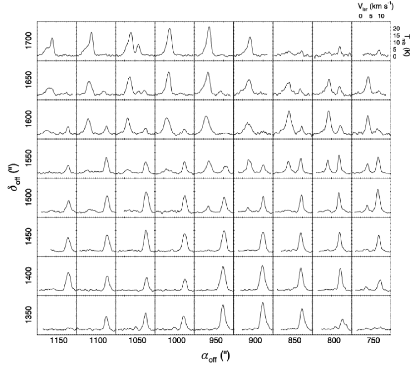
Out of the 4258 observed points, significant ¹²CO(1-0) emission was detected from 3392 of them, corresponding to a detection rate of $\sim 80\%$. In Figure 1, a sample of reduced ¹²CO(1-0) spectra, taken towards the north-western region of our VMR-D map, is shown. Despite this part of the grid is relatively small, it is representative of the velocity field complexity that characterizes this cloud. In the case of the ¹³CO(2-1) line the points showing significant emission at our sensitivity level are 648 out of 2393 ($\sim 27\%$).

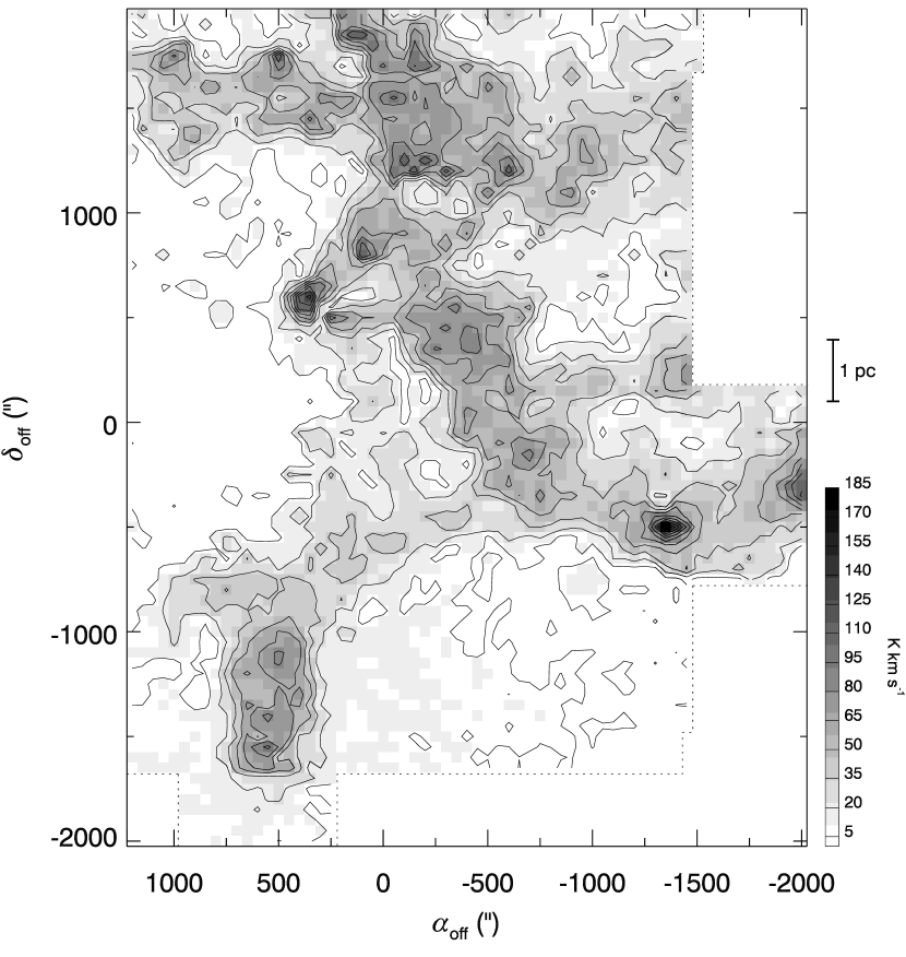
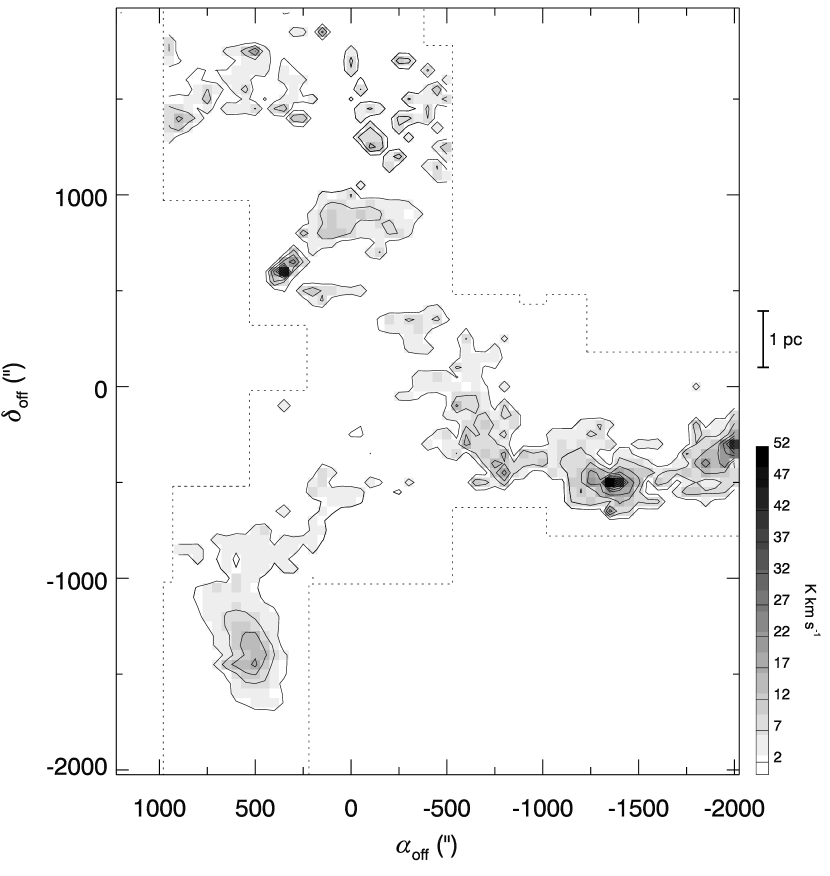
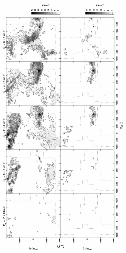
The bulk of the emission falls in the range $V_{lsr}=-2\div 20$ km s^-1 for the ¹²CO(1-0) line and $V_{lsr}=0\div 14$ km s^-1 for the ¹³CO(2-1) line, as shown in Figure 2, consistently with WB99 and YA99. The total intensity of the ¹²CO(1-0) and ¹³CO(2-1) emission, i.e. $\int T_{mb}~{}dv$ integrated from -2 to 20 km s^-1, are represented in grey-scale in Figure 3 and Figure 4, respectively.

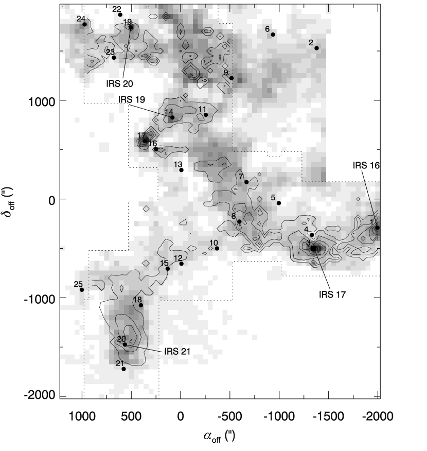
The ¹²CO(1-0) map in Figure 3 evidences a complex clumpy and filamentary structure displaying cavities of various sizes. The analysis of the velocity components, based on the channel maps and the vel-pos diagrams presented in Section 3.3, helps us in separating the various emitting regions. Here we limit ourselves to sketch the main characteristics of the cloud shape, using the locations of the bright far-IR sources in the field as reference points (see Figure 5):

• A large region in the northern part ($-1500\arcsec\lesssim\alpha_{off}\lesssim+1200\arcsec$, $+1100\arcsec\lesssim\delta_{off}\lesssim+1950\arcsec$) characterized by a strong, distributed emission. The coincidence between the position of IRS 20 and the most intense peak in this part of the map is evident.

• A central NE-SW region ($-2000\arcsec\lesssim\alpha_{off}\lesssim+500\arcsec$, $-750\arcsec\lesssim\delta_{off}\lesssim+1000\arcsec$) approximately elongated from the location of IRS 19, associated with a bright peak of integrated emission, to that of IRS 17 (the strongest peak in the whole map) and IRS 16, at the western boundary. This emitting region separate three zones, east, west, and south of it, respectively, characterized by an evident lack of emission and determining an arc-like appearance for the gas.

• An apparently compact structure in the south-eastern part of the map ($-250\arcsec\lesssim\alpha_{off}\lesssim+1050\arcsec$, $-1800\arcsec\lesssim\delta_{off}\lesssim-800\arcsec$), hosting IRS 21. This region contributes also to form the southern arc of molecular gas.

The distribution of ¹³CO(2-1) emission closely follows that of the more intense ¹²CO(1-0), as can be easily seen in Figure 4 and especially in Figure 5, in which, to highlight the correlation between the emission of the two lines, we superimpose the levels of the latter on the grey-scale map of the former. The ¹³CO(2-1) traces the densest parts of the ¹²CO(1-0) map, and its peaks coincide with those of the ¹²CO(1-0), except for the main peak in the south-eastern region. The northern region of the map is characterized by a number of isolated peaks, some of which are also recognizable in the ¹²CO(1-0) map.

In Figure 5 the positions of 25 IRAS PSC sources with fluxes increasing with wavelength ($F_{12}<F_{25}<F_{60}$) are also overplotted. Among these objects, there are also IRS 16, IRS 17, IRS 19, IRS 20, IRS 21, characterized by the further constraint $F_{25}>2.5$ Jy, recognized as intermediate mass YSOs by Liseau et al. (1992), and associated to embedded young clusters (Massi et al., 2000, 2003). Incidentally, a search for objects with increasing fluxes in the MSX Point Source Catalog (Egan et al., 2003) provided only four sources, coinciding with IRS 16, IRS 17, IRS 19, IRS 20. The reason for this small number of selected objects with respect to the IRAS archive query probably lies in the different extension of the spectral range observed.

Typically, all these sources are found in the densest parts of the cloud, and in most cases their locations follow the arc-like morphology of the gas. This is suggestive of a star formation process triggered by the effects of expanding shells driven, e.g., by nearby massive young stars or supernova remnants. In Section 3.4 we shall explore in some detail this possibility.

3.2 Gas physical properties

The present observations have been also used to derive some physical properties of the emitting gas. As a first approximation, the column density of the molecular gas traced by the thermalized and optically thick ¹²CO(1-0) line can be determined by means of the empirical formula

$$N(\mathrm{H_{2}})=(2.3\pm 0.3)\times 10^{20}\int T_{mb}(^{12}\mathrm{CO})\,dv~{}~{}(\mathrm{cm^{-2}})\,,$$ (1)

which is based on a galactic average factor (Strong et al., 1988). The molecular mass can be derived by the relation

$$M_{gas}(^{12}\mathrm{CO})=\mu~{}m_{\mathrm{H}}\sum\left[d^{2}~{}\Delta\alpha~{}\Delta\delta~{}N(\mathrm{H_{2}})\right]\,,$$ (2)

(see, e.g., Bourke et al., 1997), where $d=700$ pc is the distance of VMR-D, $(d^{2}\Delta\alpha\Delta\delta)$ is the size of the emitting area at the observed position, $m_{\mathrm{H}}$ is the mass of a hydrogen atom, and $\mu$ represents the mean molecular mass. Adopting a relative helium abundance of 25% in mass, $\mu=2.8$ and the derived cloud mass is $M_{gas}(^{12}\mathrm{CO})=1.5\times 10^{4}$ M_☉. The quite large relative error on the distance estimate, $\Delta d=200$ pc, dominates the total uncertainty affecting this value ($\Delta M/M\sim 50\%$), although it is necessary to clarify that the errors implied in the assumptions underlying this calculation probably exceed and dominate this amount. This value represents only a small fraction ($\sim$ 2.5%) of the mass reported by YA99 for the whole complex, i.e. an area of $\sim 100$ deg², because this is the mass of only a small part of one out of four clouds. Note also that VMR-B strongly contributes to the determination of the mass of the whole complex (see Equation 2), being three times more distant than the other clouds and showing a similar angular extension.

A different and more rigorous method to derive the column density relies on the simultaneous observations of the two lines, exploiting their different optical depth. As a first step the excitation temperature is estimated from the peak temperature of the ¹²CO(1-0) emission, indicated with $T_{\mathrm{R}}(^{12}\mathrm{CO})$, assuming LTE conditions and $\tau\gg 1$ (e.g., YA99, ):

$$T_{ex}=\frac{5.53}{\ln\{1+5.53/[T_{\mathrm{R}}(^{12}\mathrm{CO})+0.819]\}}\>.$$ (3)

The peak strengths were derived by gaussian fits to the ¹²CO(1-0) line profiles. Often, these show very complex profiles in this region: in these cases, we fitted only the component corresponding in velocity to the ¹³CO(2-1) feature, that generally shows only a single component. Assuming that the excitation temperature is the same also for ¹³CO we then determined the optical depth of the ¹³CO(2-1) per velocity channel by means of the relation:

$$\tau_{v}(^{13}\mathrm{CO})=-\ln\left\{1-\frac{T_{v}(^{13}\mathrm{CO})}{10.58}\left(\frac{1}{\exp(10.58/T_{ex})-1}-0.02\right)^{-1}\right\}$$ (4)

and the corresponding column density by means of the relationship (e.g., Bourke et al., 1997)

$$N(^{13}\mathrm{CO})=1.21\times 10^{14}\frac{(T_{ex}+0.88)\exp(5.29/T_{ex})}{1-\exp(-10.58/T_{ex})}\int\tau_{v}(^{13}\mathrm{CO})~{}dv\,$$ (5)

Finally, after N(H₂) is derived from $N(^{13}\mathrm{CO})$ assuming a ¹³CO abundance ratio of $7\times 10^{5}$ (Dickman, 1978), the molecular mass is calculated in the same way as for ¹²CO(1-0), amounting to $M_{gas}(^{13}\mathrm{CO})=1.2\times 10^{3}$ M_☉.

Given the undersampling of ¹³CO(2-1), a twofold bias (acting in different directions) affect the mass determination obtained through this line. On the one hand, some emission in this line is undoubtedly lost and hence unaccounted for in the total mass determination, but on the other hand, being ¹³CO(2-1) less beam-diluted than ¹²CO(1-0), then the excitation temperature as derived from ¹²CO(1-0) peak main beam temperature is underestimated (because of the smaller beam filling factor), causing an overestimate in the derived column densities.

In order to compare the LTE method results with those obtained by applying Equation 2, we calculated the mass traced by ¹²CO(1-0) considering only those positions showing detectable ¹³CO(2-1) emission; we found $M^{*}_{gas}(^{12}\mathrm{CO})=4.8\times 10^{3}$ M_☉.

Both the $M_{gas}(^{12}\mathrm{CO})$ and $M_{gas}(^{13}\mathrm{CO})$ masses are comparable to those obtained for the Orion molecular cloud which possesses similar characteristics from the point of view of the star formation activity. Of course, the comparison has to be performed taking into account both different angular size and distance of the two clouds. Mapping in ¹²CO(1-0) an area of 29 deg² in Orion A and of 19 deg² in Orion B, both located at 560 pc (Genzel & Stutzki, 1989), Maddalena et al. (1986) derived $M_{A}=1\times 10^{5}$ M_☉ and $M_{B}=9\times 10^{4}$ M_☉, respectively. Subsequently Cambrésy (1999) derived, from a visual extinction analysis of the whole cloud, a total mass $M_{AB}=3\times 10^{5}$ M_☉. Finally, a mass estimation of Orion A through ¹³CO emission, although considering the $J=1-0$ transition, has been provided by Nagahama et al. (1998), that found $M_{A,13}=5.4\times 10^{4}$ M_☉. Considering then the observed areas, these values appear consistent with those estimated for VMR-D.

3.3 Velocity structure

In Figures 6 and 7 we present the maps, for both lines, of the integrated intensity taken in velocity intervals of 2 km s^-1 and in steps of the same amount. These velocity channel maps clearly show how the emission detected in different locations is contributed by multiple velocity components. In Table 1 the characteristic velocity ranges for the main areas of the maps are summarized.

The ¹³CO(2-1) channel maps, in particular, allow us to better recognize the main velocity components of the densest regions. For example, the emission from the northern part of the map appears clearly separated into two components: one in the $V_{lsr}\simeq 0\div 4$ km s^-1 range, and the other in the $V_{lsr}\simeq 6\div 12$ km s^-1 range.

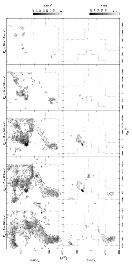
Due to the large number of observed positions, as well as the geometrical regularity of the grid (in particular for the ¹²CO(1-0) transition), we can extract vel-pos diagrams, once an offset in $\alpha$ or $\delta$ is given and the observed spectra along the given strip of the map are considered. Here we present 24 declination vs velocity ¹²CO(1-0) stripes with a fixed $\alpha_{off}$ spanning the range from $\alpha_{off}=+950\arcsec$ to $\alpha_{off}=-1450\arcsec$ (i.e. the location of IRS 17) in steps of 100″ (Figure 8), that visualize the velocity field across the cloud. In principle the same could be done for the ¹³CO(2-1) line, but at our sensitivity level the vel-pos diagrams do not add further important information so that here we omit them.

Many clump-like structures are visible in these diagrams, confirming that VMR-D possesses a high degree of inhomogeneity as will be discussed in Section 4. Several cases of strong line broadening are also detectable in correspondence to the brightest emission peaks, as for example at $\alpha_{off}=+50\arcsec$ or $\alpha_{off}=-1350\arcsec$, confirming the probable presence of outflows.

The appearance of arc-shaped structures in these diagrams can be explained either by the presence of two Galactic velocity components corresponding to gas located at different distances or by the action of expanding shells. In particular, this kind of structure is detectable in the regions $+750\arcsec\lesssim\alpha_{off}\lesssim-150\arcsec$ and $-1800\arcsec\lesssim\delta_{off}\lesssim-500\arcsec$ (southern part of the map), and $+350\arcsec\lesssim\alpha_{off}\lesssim-750\arcsec$ and $+400\arcsec\lesssim\delta_{off}\lesssim+1800\arcsec$ (northern part of the map).

The first hypothesis implies extremely different kinematical distances ($\sim 1$ kpc) between the two emitting components, an occurrence indicating the presence of uncorrelated clouds along the same line of sight. The other possibility of the shell expansion is intuitively suggested by the arc-like shapes (in Figure 8 we draw ellipses to show four possible cases), even if this can be also justified by simply invoking the internal motions of the cloud, a scenario that seems more appropriate as will be discussed in next section.

3.4 Expanding shells

The presence of arc-like features in both $\alpha-\delta$ (Figures 3, 4, 5) and vel-$\delta$ maps (Figure 8) of VMR-D region could be interpreted as a signature of possible expanding shells, a phenomenon that is often related with star forming activity.

To explore this possibility we considered the available information on the distribution of the known OB stars and Hii regions in the VMR-D field, that are shown in Figure 9 along with the spatial distribution of the gas. Three arc-like molecular structures are marked with dashed lines, but only in the case of the eastern arc we could guess an association with clear driving sources candidates. A possible projective correspondence can be established between the Gum 18 Hii region (Gum, 1955) and this arc, that could be tentatively related to it, but not for RCW 35 (Rogers et al., 1960). However, the centroids of the two structures do not coincide and the distance of Gum 18 is unknown. In addition, the OB stars V* OS Vel and CD-43 4690 are not far from the apparent centroid of the molecular arc, but their distances ($1.7\pm 0.3$ kpc in both cases, Russeil, 2003) are inconsistent with that estimated for VMR-D, so that we conclude that they cannot be responsible of the arc-like morphology of the gas. Similar considerations apply in the case of the possible association between the southern arc and the location of HD 75211 ($d=1.2$ kpc, Savage et al., 1985).

By simple models, describing the expansion of a Hii region and the fragmentation of the shocked dense layer surrounding it, it is possible to estimate the timescales involved in the hypothesis that the shell driving sources are Hii regions. The relation between the radius $R$ of the shell, expanding in a homogeneous and infinite medium, and its lifetime is

$$t_{dyn}=0.559\times\frac{R_{0}}{c_{\mbox{{ii}}}}\left[\left(\frac{R}{R_{0}}\right)^{7/4}-1\right]~{}\mathrm{Myr}$$ (6)

(Spitzer, 1978), where $R_{0}$ is the Strömgren sphere radius (in pc), and $c_{\mbox{{ii}}}$ the isothermal sound speed in the ionized region (in km s^-1). Being the molecular arc $\sim 1000\arcsec$ in radius, the corresponding spatial scale is $R\simeq 3.4\pm 1.0$ pc at the estimated distance of VMR-D, where the uncertainty is related to the distance. For a star emitting $10^{49}$ ionizing photons per second, we find $R_{0}=0.677~{}n_{3}^{-2/3}$ pc, where $n_{3}=n_{0}/(1000~{}\mathrm{cm}^{-3})$ and $n_{0}$ is the ambient density. Assuming the sound speed $c_{\mbox{{ii}}}=10$ km s^-1 and varying the density in the range $n_{0}=300\div 3000$ cm^-3, we find $t_{dyn}\sim 0.2\div 1.1$ Myr. The scaling of the age with the density is shown in Figure 10 for different estimates of the distance.

Considering now the Whitworth et al. (1994) model describing the fragmentation of the molecular gas under the action of an expanding Hii shell, it is also possible to determine the time elapsed before the onset of this phenomenon. For the considered star this model gives

$$t_{frag}=1.56~{}c_{.2}^{7/11}~{}n_{3}^{-5/11}~{}\mathrm{Myr}$$ (7)

where $c_{.2}=c_{s}/(0.2~{}\mathrm{km~{}s}^{-1})$, and $c_{s}$ is the sound speed in the molecular gas, an important parameter of the model we chose in the range $c_{s}=0.2\div 0.6$ km s^-1.

Because both fragmentation and star formation appear to be already in progress, the relation between these two times have to be $t_{dyn}>t_{frag},$ and this happens when $t_{dyn}\gtrsim 8\times 10^{5}$ yr and $n_{0}\gtrsim 1600$ cm^-3, if we consider the preferred values $d=700$ pc and $c_{s}=0.2$ km s^-1. The effect of a different distance is also shown in Figure 10.

We note that these timescales are consistent with the age of the cluster formation activity in this region, estimated to be within $1\div 6$ Myr by Massi et al. (2006a). This makes possible that both arcs and the star formation activity in them are caused by the expansion of Hii regions. However, since no clear excitation source candidates have been found in the vicinity of the arc centers, we cannot exclude different possible origins for the shells, such as for example stellar winds from a previous generation of young stars.

Despite another possibility is suggested by the well-known Vela SNR, apparently interacting with the whole VMR on larger scales (see Figure 1 in Moriguchi et al., 2001), a correlation with the southern arc in VMR-D is far from clear. Furthermore, considering the possible connection between this molecular arc and its star formation activity, there is a clear inconsistency between the age of the YSOs and that estimated for the Vela SNR ($t_{\mathrm{SNR}}\simeq 10^{4}$ yr, see, e.g., Moriguchi et al., 2001). Two further remnants, SNR 266.3-01.2 and SNR 260.4-03.4, are too far for being responsible for the peculiar morphology of the investigated region.

In this respect, the hypothesis that the fluidodynamic evolution of the gas can be responsible of the observed filamentary condensations can not be rejected.

As mentioned above, also the analysis of the cloud velocity field can provide useful information about the presence and the physical properties of possible expanding shells. For example, the shell-shaped structure highlighted in Figure 8 at $\alpha_{off}=+350\arcsec$ can be associated, due to its spatial location, to the southern arc identified in the $\alpha-\delta$ map. It is characterized by a peak separation $\Delta V_{lsr}\simeq 7$ km s^-1, corresponding to an expansion velocity $V_{exp}\simeq 3.5$ km s^-1. Adopting a spherical symmetry, we estimate a mean radius $R_{sh}\simeq 5.5$ pc and a corresponding dynamical age $t_{dyn}\simeq 1.5$ Myr, a value consistent with the possible timescales calculated above for an expanding Hii region. A rough estimate of the kinetic energy can be also obtained by adopting the assumption inspiring the Equation 2 and considering the expansion velocity of each spectral component. In this way we find $E_{kin}\simeq 2.3\times 10^{47}$ erg, a value comparable, for example, with the kinetic energy of a Hii region possessing the same radius and age (Spitzer, 1978). The issue of the identification of a driving source for this shell remains open, as already discussed when we examined the corresponding arc observed in the $\alpha-\delta$ map.

Another shell-like structure is well recognizable in the northern part of the vel-pos diagrams, best visible at $\alpha_{off}=-450\arcsec$. With considerations similar to the previous case, we find $V_{exp}\simeq 4.5$ km s^-1, $R_{sh}\simeq 7$ pc, $t_{dyn}\simeq 1.5$ Myr, and $E_{kin}\simeq 5.4\times 10^{47}$ erg. Also in this case the identification of a possible driving source is uncertain: some IRAS red sources, namely those identified as 9, 11, and 14 in Table 2, are located in the neighborhoods of the shell, but these objects might be presumably the product of a star forming activity triggered by an expanding shell, rather than the cause of it. In conclusion, the ages derived for these two candidate shells are similar, and support the hypothesis of a synchronous intermediate-mass star formation in this cloud, originated by a strong compression of the gas due to the associated shocks. For this process we suggest an upper limit in timescale of $t\simeq 1.5$ Myr.

In Figure 8 two further arc-shaped structures have been marked with solid lines, around $\alpha_{off}=-650\arcsec$ and $\alpha_{off}=-750\arcsec$, respectively. Although less evident than the cases considered above, these shapes support the hypothesis of a coupling between the arcs recognized in the integrated intensity maps (in these cases, the western and the southern one, respectively) and those present in the vel-pos diagrams.

3.5 Search for outflows

Since several positions in the map show a clear broadening of the line profile (see, e.g., the diagram at $\alpha=-1350\arcsec$ of Figure 8) we studied these positions in more detail because this is a typical signature of the presence of energetic mass outflows (see, e.g., Bachiller, 1996).

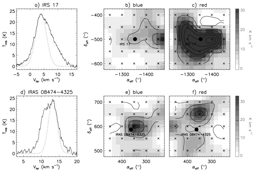
To this aim we considered the locations of the 25 IRAS sources shown in Figure 5 and quoted in Table 2, carrying out a systematic search for outflows in the ¹²CO(1-0) line toward these objects. The detection method is the same as adopted by WB99: a gaussian is fitted to the upper part of a spectral feature, centered on the line peak, and at the same intensity; the smaller of the two intervals between the peak velocity and the velocities at half maximum is taken as the HWHM of the fitting gaussian. When the profile wings significantly exceed the gaussian wings, the presence of an outflow is inferred and the blue and red components are obtained by integrating the difference $T_{mb}-T_{fit}$ between the half maximum of the gaussian and the velocity where the line wing fades into the noise. In Figure 11, panels $a$ and $d$, we show, as an example, the ¹²CO(1-0) spectrum of the pointings closest to the IRS 17 and IRAS 08474-4325 (identified with 3 and 17 in our list, respectively) locations, with the fitting gaussian determined as described above. In panels $b$-$c$, $e$-$f$ the intensities of the blue and red components, in the neighborhoods of these two sources are represented in greyscale.

In seven cases the presence of one or more additional spectral components blended with the main feature made impracticable a clean detection of any outflow that might be present. This difficulty restricts our sample, even if it remains still meaningful in the perspective of providing good target candidates for future APEX and ALMA observations.

In 13 out of the remaining 18 cases, we detected a possible outflow, as summarized in Table 2: column 9 contains a flag indicating the result of the detection, column 11 the width of the velocity range subtended by the wings, and column 12 the offset of the wing maximum emission from the map pixel in which the source falls. Note that in two cases only one wing is detected and that when the detection flag “Y” is followed by an asterisk, a gaussian fit of a secondary (but well-separated) component has been subtracted to correctly estimate the wing intensities.

Unfortunately, the complexity of the ¹²CO(1-0) spectra in this region makes sometime difficult an accurate detection of the wings by simply applying the WB99 method. The example of IRS 17 in Figure 11, panel $a$, is illustrative: the temperature peak does not stand in the center of the feature, so that a much larger amount of emission is recognized in the red wing. Instead, the blue wing seems better suited to be interpreted as an outflow. Vice versa in the case of IRAS 08474-4325: the two cases discussed have been shown in Figure 11 just to highlight the differences between a reliable detection of outflows (blue wing of IRS 17 and red wing of IRAS 08474-4325), and more controversial cases (red wing of IRS 17 and blue wing of IRAS 08474-4325). The latter are indicated in Table 2 with a dagger mark.

Because our work was not focused on the study of the outflows, we remark that the grid spacing of 50″ is quite coarse for a detailed description of the outflow morphology, and a larger integration time would have been required for each spectrum to better disentangle the wing tails from the noise. These problems are evident in comparing our results with those obtained by WB99 for the three objects in common with our sample (associated with IRS 17, IRS 19, IRS 20 respectively): in our case the wing width is significantly smaller than found by WB99, ranging from 32% (blue wing of IRS 20) of their values to 71% (red wing of IRS 17).

Furthermore, considering that ¹³CO(2-1) observations are too noisy for a similar analysis, it is almost impossible to exploit them for a quantitative study of the outflow physical properties. In any case our analysis significantly improves the outflow statistics in the observed region, from three to 13 objects, providing a larger sample of targets for future higher resolution observations.

4 Cloud decomposition

To characterize the structure of VMR-D and the distribution of its velocity components in a quantitative way we applied cloud decomposition techniques to our data, a tool typically adopted to study possible hierarchies in the molecular cloud structure. In particular, we adopted the 3D version of the CLUMPFIND (hereinafter CF) algorithm (Williams et al., 1994), running on a $\alpha$-$\delta$-$v$ cube containing all the reduced spectra for each line. Important adjustable parameters in the CF scanning procedure are the radiation temperature threshold $T_{min}$ and the level increment $\Delta T$, the first one being generally set slightly above the noise fluctuations. This is an important point that requires accurate tests because larger and smaller thresholds involve the loss of faint peaks and the inclusion of noise peaks, respectively. The second parameter $\Delta T$ controls the separation of close peaks, as clearly discussed in Brunt et al. (2003).

A large number of tests have been run on the ¹³CO(2-1) data cube, which is characterized by a smaller number of features and a reduced diffuse emission, two characteristics that allow a better control and verification of the reliability of the clump assignments. To obtain a convenient reduction of the noise effect and to ensure some stability to the results, the spectra were preliminarily resampled in velocity by a factor of 5.

Exploring the input parameter space, we noted that the choice of the parameter set can produce not only systematic (as those described above), but also random effects. These are particularly evident, for example, in large clumps corresponding to a single bright line, that are sometimes decomposed in two or more clumps, an effect that is illustrated in Figure 12. We verified that, adopting a different set of parameters, the clump could appear as single, the price being that some other cases, previously recognized as single, now appear as separated. This experience suggests that the tuning of the parameter values is critical with respect to the number of detections. This kind of problems in cloud decomposition with CF have been extensively discussed in Brunt et al. (2003), Rosolowsky & Blitz (2005), and Rosolowsky & Leroy (2006).

In this work, the relatively low number of detected clumps suggested us a very simple approach based on the careful inspection of a large number of CF outputs. First of all, we ran CF adopting a parameter set ensuring a good detection of the features, i.e. a $T_{min}$ value as low as possible, although above the noise limit, and a similar value also for $\Delta T$, to minimize the effect of noise fluctuations affecting the spectra. Both values have been set to 2 K, corresponding to $\sim 3\sigma$ in our map. In this way, the cataloged emission accounts for the 66% of the total emission in the ¹³CO(2-1) map, as shown in Figure 2.

The obtained clump list has then been analyzed looking for those objects that, despite they are quite close in the $\alpha$-$\delta$-$v$ space, clearly appear as spuriously splitted by CF. We merged together these clumps to obtain a final clump distribution as free as possible from the most apparent misinterpretations of CF. In this way, we do not claim to determine the “true” clump distribution in the cloud, but we believe that the census resulting from our clump merging method is more reliable than the simple CF output.

Our experience in analyzing the clump merging suggested a set of constraints that have been included in an automatic merging algorithm. In fact, we merged only clump pairs whose centroids satisfy all the following criteria: i) both distances in $\alpha$ and $\delta$ are less or equal to 3 grid elements (corresponding to a spatial scale of $\sim 0.5$ pc); ii) the difference between the central velocities is less than or equal to 3 channels (i.e. $\Delta v\leq 0.9$ km s^-1, after resampling); iii) the $\alpha$-$\delta$-$v$ space total distance $d=\sqrt{\Delta\alpha^{2}+\Delta\delta^{2}+\Delta v^{2}}$ is less than or equal to 5 volume pixels. In this context the pairs showing a spatial discontinuity in their emission have been taken as separated.

After this procedure the number of detected ¹³CO(2-1) clumps decreased from 67 to 49 clearly modifying the resulting mass spectrum, with the total detected mass remaining obviously unchanged.

The list of these clumps, along with their coordinates, velocity centroids, radii, masses, corresponding virial masses and optical depths is presented in Table 3.

The clump masses have been evaluated assuming the LTE condition, as we did in Section 3.2 for the whole cloud, so that the total mass assigned to these clumps amounts to 845 M_☉, corresponding to the 77% of the whole $M_{gas}(^{13}\mathrm{CO})$ calculated.

The virial masses in column 8 are obtained from the observed radius $R$ and velocity dispersion $\Delta V$ under the hypothesis of constant density (MacLaren et al., 1988)

$$M_{vir}=210\left(\frac{R}{\mathrm{pc}}\right)\left(\frac{\Delta V}{\mathrm{km~{}s}^{-1}}\right)^{2}\>.$$ (8)

For density radial profiles as $\rho\propto r^{-1}$ and $\rho\propto r^{-2}$ the multiplicative constant decreases to 190 and 126, respectively.

The optical depth is calculated along the line of sight of the clump centroid using Equation 4. We list in column 9 the optical depth at peak velocity, and in column 10 the integral of this observable over the velocity channels assigned to the considered clump. Note that for the clump VMRD43 the maximum and the integrated optical depth are significantly higher than others, because of the similarity of ¹²CO(1-0) and ¹³CO(2-1) peak temperatures.

For clumps at the boundary of the observed zone a flag “X” is added to indicate that the quoted clump mass value actually is a lower limit.

Comparing these results with the list of 29 dust cores presented in MA06 and obtained applying the 2D version of CF to 1.2 mm continuum observations of VMR-D at the SEST, we searched for possible associations between ¹³CO(2-1) and dust condensations, adopting as a criterium the correspondence between the dust core centroid and one of the map points assigned by CF to a gas clump. We found 16 cases that are reported in Table 3. Note that in this way the information on the velocity field, allowing to separate possible multiple components along the line of sight, can induce the association between two gas clumps and a group of dust cores (see, for example, the clumps VMRD36 and VMRD37). On the other hand, by comparing the two lists in the opposite way, we can note that only the dust cores MMS10 and MMS11 are not associated to ¹³CO(2-1) clumps. This implies that, in general, the continuum emission is able to track even denser zones than ¹³CO(2-1) line, and in fact, considering the gas clumps associated to a group of MA06 dust cores, we find that the total mass is larger or quite similar to the mass traced by dust. The average value of their ratio is in fact $M_{gas}$(line)$/M_{gas}$(continuum)$=1.44\pm 0.11$, while the median of the distribution is 0.96. Furthermore, the clumps that remain unassociated have intermediate or small masses ($M\leq 20$ M_☉). Finally, in Table 3 the associations with the IRAS PSC sources of Table 2 are also indicated: 22 out of 25 objects fall in the area observed in ¹³CO(2-1), and the locations of 15 sources (among which are the five IRS objects of Liseau et al., 1992) can be associated with the recognized clumps.

The derived mass spectrum is shown in Figure 13, with Poisson error bars, along with the spectrum resulting from the original CF output. For nine clumps we can only give a lower limit to the mass because they are bounded by our map limits. This effect is particularly important in the case of the large clump hosting IRS 16 (clump VMRD1 in Table 3). The minimum mass detectable and the completeness limits, calculated as in Simon et al. (2001) by setting a 10$\sigma$ confidence level (see also Bains et al., 2006), and estimated in 0.19 M_☉ and 0.98 M_☉, respectively, are also shown.

A linear least-squares fit of the distribution of the masses above the completeness limit provides an estimate of the $\mathrm{d}N/\mathrm{d}M\propto M^{-\alpha}$ law exponent, which has been found to be $\alpha=2.0\pm 0.3$ for the “corrected” sample and $\alpha=1.8\pm 0.3$ for the original CF output (see Figure 13). In general, dealing with a relatively small sample of clumps, the spectral index can be also sensitive to the particular choice of the bin size. It was set here to be 0.2 (in logarithmic units), after verifying the stability of the resulting slope with respect to other possible choices. By varying, as in Bains et al. (2006), the bin size in the range of $\pm 10\%$ we obtain slopes that always fall within the associated error.

Concluding this discussion about the ¹³CO(2-1) clump mass distribution, we remark that the observed values are significantly below those calculated with the virial theorem: these two values often differ by one order of magnitude, even considering different internal density distributions. Interestingly, the same result is found for the millimeter dust core distribution by MA06, who indicate two possible confining mechanisms related either to external pressure or to toroidal magnetic fields, excluding the first one. The hypothesis that these clumps, or part of them, are gravitationally bound cannot be excluded a priori if they are collapsing, as could be suggested by the presence of associated IRAS sources (see Table 3). However a particular trend in the mass ratio cannot be recognized in these cases, so that it remains difficult a definite conclusion about the collapsing or dispersing status of these clumps.

In applying the CF algorithm to the ¹²CO(1-0) line data cube, the large number of blended components, as well as the presence of a diffuse component in a large fraction of the map, make the decomposition much more difficult and the definition of “clump” more uncertain. Other difficulties are related to the optical depth of this line that can be affected by self-absorption. However, the ¹²CO(1-0) observations are characterized by a better sampling with respect to ¹³CO(2-1), approximately 1 beam and 2 beams, respectively. In this situation it is actually difficult to discern which line produces the most reliable slope for the mass spectrum.

Even for the ¹²CO(1-0) line the previous merging procedure was applied, obtaining 168 objects from the original 275 ones. The cataloged emission in clumps accounts for the 84% of the total emission in the ¹²CO(1-0) map.

It is noteworthy that the positions of the ¹³CO(2-1) clumps and the MA06 dust cores coincide with those of ¹²CO(1-0) clumps, suggesting that this line, although optically thick, can be anyway used to reliably track the gas clumps.

The method used to determine the ¹²CO(1-0) clump masses is based on Equation 2: even if this empirical relationship can be questioned in the case of small-scale structures, it is the only way to exploit the ¹²CO(1-0) data for mass determinations and is often used to derive the clump mass spectra down to the lower masses (see, e.g., Heithausen et al., 1998). The resulting mass spectrum presented in Figure 14 shows, in the case of the merged sample, a “flat” central part and an approximately linear decrease in the large mass limit of the distribution. The minimum mass and the completeness limits are, respectively, 2.9 M_☉ and 12.6 M_☉. The spectral indexes obtained with and without merging are significantly different, $\alpha=1.3\pm 0.1$ and $\alpha=1.8\pm 0.1$, respectively. While the second value is consistent with the corresponding index derived for ¹³CO(2-1), those obtained after merging are clearly different. It is plausible that the high optical depth of ¹²CO(1-0)makes much more difficult to define the actual borders of clumps.

Note that the spectral indexes found in VMR-D for the corrected clump lists agree with those reported in the literature for molecular line observations ($1.3\leq\alpha\leq 1.9$, see, e.g., Mac Low & Klessen, 2004), and are smaller than the typical slopes of the stellar IMF (e.g., $\alpha\sim 2.35$ in Salpeter, 1955).

The slopes obtained here seem also comparable with the power-law index $\alpha_{dust}=1.45\pm 0.2$ reported in MA06 if we consider the quoted errors and the fact that the dust continuum observations completely include those high-mass clumps which are only partially contained in our map (in particular the massive clump hosting IRS 16).

The difference found between the ¹³CO(2-1) and the dust indexes could be due to opacity effects that in the case of the more massive clumps can be considerable. This corresponds to an underestimate of the larger masses and then to a steeper slope in the mass spectrum. For another similar case in which $\alpha_{gas}>\alpha_{dust}$, see Bains et al. (2006).

Considering now the mass-radius relation shown in Figure 15 we can further extend the discussion in MA06 about the slope of this relation. In that work the exponent of the $M\propto R^{x}$ relation has been evaluated $x=1.7$, with this value decreasing when the masses are determined by adopting two different temperature-opacity values for cores with and without associated IRAS sources. Here on the other hand, with reference to a weak linear behavior in the bi-logarithmic plot, we find significantly different slopes in the case of ¹²CO(1-0) and ¹³CO(2-1) clumps: $x=2.5\pm 0.3$ and $x=1.9\pm 0.5$, respectively. This discrepancy can result from all the uncertainties involved in the two derived mass distributions, in particular from the different optical depths. The ¹³CO(2-1) value appears more consistent with that of MA06, both suggesting the presence of Bonnor-Ebert clumps. Conversely, the slope derived from ¹²CO(1-0) is more consistent with a turbulent fragmentation scenario (see, e.g., Elmegreen & Falgarone, 1996).

Another relevant information resulting from the cloud decomposition procedure is the internal velocity dispersion $\sigma$ of each clump that can be used to examine its scaling relation with the radius $R$. This is generally reported as $\sigma\propto R^{\beta}$ (empirically derived by Larson, 1981), with $\beta$ varying between 0.2 and 0.5 (see, e.g. Schneider & Brooks, 2004), the most quoted value being $\beta=0.4\pm 0.1$ (Mac Low & Klessen, 2004, and references therein). In Figure 16 we present the scatter plot of the velocity dispersion vs radius for the clumps observed in the two lines. If we fit the data with a linear regression, the resulting slope is $\beta=0.4\pm 0.1$ for ¹²CO(1-0), and $\beta=0.4\pm 0.2$ for ¹³CO(2-1). These values are not far from $\beta=0.5$, that is the value corresponding to the virial equilibrium, a condition implying equipartition between self-gravity and turbulent energies. The same equilibrium is consistent with the slope $x=1.9$ we find for the mass vs radius relation for the ¹³CO(2-1).

On the other hand, other authors (see, e.g., Mac Low & Klessen, 2004, and references therein) consider a non-static scenario and explain this value with the presence of supersonic turbulent cascades that appear to be more consistent with the results we obtained above on the gravitational stability of the ¹³CO(2-1) clumps. Finally, it is noteworthy that $\beta=0.5$ is also the value determined in two surveys of the galactic plane carried out by Dame et al. (1986) and Solomon et al. (1987).

5 Summary

In this work we examined the CO distribution in one of the most interesting parts of the Vela Molecular Ridge (i.e., a $\sim 1\arcdeg\times 1\arcdeg$ area of Cloud D) with unprecedented spatial resolution ($\sim 50\arcsec$). The main reasons of interest for this cloud are its star formation activity and its location in the galactic plane. VMR-D is in fact the nearest massive star forming region with this galactic position.

The millimeter line observations of the CO isotopes in VMR-D, carried out at ESO-SEST, revealed a complex spatial and spectral behavior down to the smallest spatial scales investigated ($\sim 1$ pc). The two rotational transitions analyzed, ¹²CO(1-0) and ¹³CO(2-1), due to their different optical depth, allowed us to probe both low and high density regions, confirming a tight link between the gas distribution and the location of the brightest point-like far-IR sources known in the field. The main filamentary structures, appearing in the integrated intensity maps, show an arc-like shape although it is not clear if this is produced by expanding shells or stellar winds, both driven by nearby young (massive) stars. If an expanding Hii region is considered, its dynamical age is compatible with that estimated for the star formation activity. Contributions from nearby known supernova remnants are excluded. Another possibility is that the observed arcs are the product of the internal cloud turbulent motions.

The analysis of the velocity field has shown several well-separated zones, emitting at different velocities and suggesting a complex structure and dynamics. In two regions, the presence of both two velocity components (separated by $\sim 3.5$ and $\sim 4.5$ km s^-1, respectively) and arc-shaped morphology in the vel-pos diagrams can be interpreted as a signature of expanding shells. These, compressing the gas, can be thought as the cause of the observed cluster formation. The evolutionary times involved in such a scenario are consistent with the star formation age of this cloud. Further arc-like structures are also present in the vel-pos diagrams which can be associated with the molecular arcs in the integrated intensity maps.

The line profiles near the bright far-IR sources often appear clearly broadened, suggesting the presence of outflows. A search for such outflows in ¹²CO(1-0) line near the IRAS red sources shows that, within the limits of resolution and noise of our observations, there are 13 candidate objects worth of further and more detailed observations for mapping their structure and accurately determining their physical parameters.

One of the immediate developments of this work will be a multi-wavelength analysis of this cloud with the aim of correlating the clustered star formation (Lorenzetti et al., 1993; Massi et al., 2000, 2006a) with the gas and dust physical conditions.

Cloud decomposition has been carried out by means of the CLUMPFIND code and subsequently corrected for spurious effects due to the misinterpretation of the random noise fluctuations in the spectra. We find that the clump mass spectra of ¹²CO(1-0) and ¹³CO(2-1) observations are different. Both values are typical for interstellar molecular clouds and, significantly, are in agreement with that obtained by MA06 for dust cores in VMR-D.

In all the investigated ¹³CO(2-1) clumps the masses have been found to be lower than the corresponding virial masses, revealing that these clumps are either gravitationally unbound or collapsing.

A power-law fit of the clump mass vs radius shows that the exponent are $x=2.5$ for ¹²CO(1-0) and $x=1.9$ for ¹³CO(2-1). Finally, a similar fit of the internal velocity dispersion vs clump radius gives a slope $\beta\sim 0.4$ in both transitions, a value suggesting either virial equilibrium or internal turbulence. The first hypothesis is however excluded when we take into account the inconsistency between observed and virial clump masses.

Table 1: Velocity ranges of the main emitting regions in VMR-D

Region	12CO(1-0)	13CO(2-1)
	(km s-1)	(km s-1)
North-East	$-2\div 12$	$0\div 4$, $6\div 12$
North-West	$0\div 6$, $10\div 18$	$4\div 10$
Center	$4\div 16$	$4\div 12$
West	$0\div 10$	$0\div 6$
South (diffuse component)	$0\div 6$	$\cdots$
South-East	$4\div 16$	$6\div 12$

Table 2: IRAS PSC sources in the observed field, with fluxes increasing from 12 $\mu$m to 60 $\mu$m, and associated outflows.

	IRAS	$F_{12}$	$F_{25}$	$F_{60}$	$F_{100}$	$L_{FIR}$	$V_{lsr}$	Outflow	Wing	$V_{\mathrm{range}}$	Offset
	name	(Jy)	(Jy)	(Jy)	(Jy)	($L_{\sun}$)	(km s-1)	(Y/N/…)		(km s-1)	(″)
1	08438-4340 (IRS 16)	13.4	56	638	1580	566	7.68	Y	blue	6.48	$(0,-50)$
									red	3.84	$(+50,+50)$
2	08447-4309	$<$ 0.25	$<$ 0.4	$<$ 4.4	36	6	11.28	…
3	08448-4343 (IRS 17)	8.7	88	327	1010	415	3.96	Y	blue	8.64	$(0,0)$
									red	8.88	$(-50,0)$
4	08448-4341	1.3	6.7	$<$ 327	$<$ 1010	258	4.20	N
5	08453-4335	$<$ 0.34	0.59	$<$ 6.4	$<$ 49	9	6.12	N
6	08454-4307	$<$ 0.25	0.36	$<$ 3.3	$<$ 39	6	2.52	Y	blue	1.92	(+100,+50)
									red	6.72	(+50,0)
7	08458-4332	1.1	2.7	18	53	20	12.00	…
8	08459-4338	$<$ 0.29	0.57	6.5	38	8	6.00	Y	blue	4.32	(-100,0)
9	08461-4314	0.69	0.79	5.9	$<$ 49	9	2.52	…
10	08463-4343	$<$ 0.29	0.49	7.4	$<$ 44	8	10.44	Y	blue	3.48	(+50,0)
									red	6.24	(+50,+100)
11	08465-4320	$<$ 0.25	$<$ 1.1	$<$ 3.5	30	6	12.00	…
12	08468-4345	0.39	$<$ 0.87	$<$ 4.8	$<$ 36	7	9.60	Y	red	6.12	(+100,0)
13	08468-4330	$<$ 0.3	0.43	3.4	$<$ 32	5	6.72	N
14	08470-4321 (IRS 19)	45	130	343	407	514	12.96	Y	blue	4.56	(0,-50)
									red	6.00	(0,-50)
15	08471-4346	$<$ 0.28	$<$ 0.5	5.4	36	7	8.16	…
16	08472-4326A	0.85	0.94	11	$<$ 407	45	12.48	N
17	08474-4325	$<$ 0.3	0.96	$<$ 16	58	15	13.20	Y	blue	8.16	(0,0)
									red	4.68	(0,+50)
18	08475-4352	$<$ 0.44	$<$ 0.45	$<$ 2.9	31	5	8.52	…
19	08476-4306 (IRS 20)	5.7	44	216	504	234	2.28	Y	blue	2.64	(0,0)
									red	4.68	(0,-50)
20	08477-4359 (IRS 21)	9	26	317	581	265	7.80	Y	blue	5.88	(+50,-50)
									red	4.44	(0,-50)
21	08478-4403	0.46	0.51	5.4	$<$ 581	56	10.20	…
22	08478-4303	$<$ 0.39	1.6	$<$ 216	$<$ 35	108	4.92	N
23	08479-4311	$<$ 0.32	0.4	$<$ 8.7	$<$ 38	8	2.52	Y	blue	3.60	(0,+50)
									red	2.52	(+50,+50)
24	08483-4305	1.5	2.5	$<$ 39	189	42	3.36	Y	blue	7.80	(+100,0)
									red	2.04	(+50,+50)
25	08484-4350	0.33	$<$ 0.56	$<$ 3.7	23	5	6.24	Y	blue	1.80	(-50,0)
									red	3.24	(-100,0)

Table 3: List of the clumps detected in the ¹³CO(2-1) line.

	$\alpha$ (2000)	$\delta$ (2000)	$V_{lsr}$	$\Delta V$	Radius	Mass	$M_{vir}$	$\tau_{V,MAX}$	$\int\tau_{V}\,dV$	Map limit	Dust	IRAS
	h  m  s	°  ′  ″	(km s-1)	(km s-1)	(pc)	(M☉)	(M☉)	(km s-1)-1			clump(s)	source(s)
VMRD1	8 45 35	-43 52 02	5.9	2.55	0.6	83	842	0.90	2.58	X	MMS1,2,3	1
VMRD2	8 45 36	-43 48 42	5.3	1.80	0.4	16	248	0.62	0.66	X	MMS1,2,3	1
VMRD3	8 46 17	-43 56 12	4.1	1.14	0.5	17	142	0.26	0.34		$\cdots$	$\cdots$
VMRD4	8 46 31	-43 54 32	2.9	1.09	0.7	48	165	0.69	0.75		MMS4	3,4
VMRD5	8 46 35	-43 54 32	5.0	1.53	0.7	70	324	0.97	2.39		MMS4,5,6	3,4
VMRD6	8 46 49	-43 50 22	4.7	1.06	0.4	9	94	0.26	0.06		$\cdots$	$\cdots$
VMRD7	8 46 54	-43 54 32	4.1	1.71	0.6	38	388	0.33	0.17		MMS5,6	$\cdots$
VMRD8	8 47 26	-43 48 42	5.6	1.11	0.4	10	99	0.32	0.46		$\cdots$	$\cdots$
VMRD9	8 47 26	-43 52 52	2.9	1.36	0.4	17	145	0.45	0.44		$\cdots$	$\cdots$
VMRD10	8 47 31	-43 52 52	4.1	0.93	0.4	8	67	0.41	0.39		$\cdots$	$\cdots$
VMRD11	8 47 40	-43 43 42	11.3	0.99	0.3	11	72	0.59	0.50		$\cdots$	7
VMRD12	8 47 45	-43 47 02	6.8	0.84	0.5	15	78	0.28	0.22		$\cdots$	$\cdots$
VMRD13	8 47 45	-43 50 22	5.0	1.31	0.4	15	143	0.42	0.71		$\cdots$	8
VMRD14	8 47 50	-43 47 52	5.9	0.77	0.4	8	46	0.22	0.21		$\cdots$	8
VMRD15	8 47 54	-43 27 52	2.0	0.73	0.2	3	16	0.34	0.42	X	$\cdots$	$\cdots$
VMRD16	8 47 59	-43 39 32	10.4	0.64	0.2	2	17	0.22	0.12		MMS7	$\cdots$
VMRD17	8 47 59	-43 25 22	2.3	0.68	0.2	3	19	0.62	0.20	X	$\cdots$	9
VMRD18	8 47 59	-43 20 22	1.1	0.50	0.2	3	12	0.78	0.60	X	$\cdots$	$\cdots$
VMRD19	8 48 03	-43 51 12	4.7	0.76	0.2	3	24	2.58	1.44		$\cdots$	$\cdots$
VMRD20	8 48 13	-43 47 02	7.7	1.62	0.3	3	143	0.28	0.16		$\cdots$	$\cdots$
VMRD21	8 48 13	-43 22 52	2.3	1.07	0.4	15	86	1.03	0.73		$\cdots$	$\cdots$
VMRD22	8 48 17	-43 17 52	1.4	1.08	0.2	5	36	0.62	0.62		$\cdots$	$\cdots$
VMRD23	8 48 17	-43 26 12	2.3	0.88	0.2	3	23	0.57	0.65		$\cdots$	$\cdots$
VMRD24	8 48 27	-43 41 12	6.5	1.69	0.3	5	201	0.48	0.11		$\cdots$	$\cdots$
VMRD25	8 48 31	-43 22 02	2.0	0.85	0.2	4	26	0.54	0.44		$\cdots$	$\cdots$
VMRD26	8 48 31	-43 25 22	2.3	0.91	0.2	6	34	0.42	0.53		$\cdots$	$\cdots$
VMRD27	8 48 31	-43 34 32	12.5	1.18	0.4	11	125	0.47	0.24		$\cdots$	11
VMRD28	8 48 40	-43 29 32	11.3	1.33	0.4	8	153	0.50	0.45		MMS8,9,12,14,15,16	14
VMRD29	8 48 40	-43 17 52	2.3	0.87	0.2	6	23	0.88	0.53		$\cdots$	$\cdots$
VMRD30	8 48 50	-43 29 32	13.1	1.07	0.5	16	123	0.39	0.20		MMS8,9,12,13,14,15,16	14
VMRD31	8 48 54	-43 15 22	2.0	0.97	0.2	8	35	0.79	0.78		$\cdots$	$\cdots$
VMRD32	8 48 59	-43 59 32	8.3	1.44	0.5	16	229	0.81	0.53		$\cdots$	15
VMRD33	8 49 03	-43 32 52	11.9	0.86	0.2	4	37	0.58	0.54		$\cdots$	$\cdots$
VMRD34	8 49 03	-43 37 52	11.9	1.69	0.2	10	143	0.54	0.71		MMS17,18	16
VMRD35	8 49 12	-43 22 02	1.4	1.27	0.3	5	93	0.37	0.52		$\cdots$	$\cdots$
VMRD36	8 49 13	-43 36 12	11.3	1.55	0.3	32	170	0.94	1.81		MMS19,20,21	17
VMRD37	8 49 13	-43 36 12	12.8	0.86	0.3	9	45	0.64	0.46		MMS19,20,21	17
VMRD38	8 49 22	-44 00 22	8.3	1.40	0.6	19	228	0.39	0.24		$\cdots$	$\cdots$
VMRD39	8 49 22	-43 58 42	7.4	1.07	0.4	8	88	1.01	0.81		$\cdots$	$\cdots$
VMRD40	8 49 26	-43 22 02	3.5	0.72	0.2	3	21	0.32	0.30		$\cdots$	$\cdots$
VMRD41	8 49 26	-43 17 02	2.6	0.90	0.3	10	59	0.28	0.37		MMS22,24	19
VMRD42	8 49 26	-43 17 02	1.7	0.85	0.2	3	26	0.26	0.23		MMS22,24	19
VMRD43	8 49 27	-44 10 22	8.9	1.57	0.7	78	365	3.55	5.50		MMS25,26,27	20
VMRD44	8 49 31	-43 20 22	7.7	1.16	0.3	4	73	0.40	0.42		$\cdots$	$\cdots$
VMRD45	8 49 31	-44 07 52	9.8	1.63	0.7	141	373	1.10	0.59		MMS23,25,26,27	20
VMRD46	8 49 49	-43 21 12	8.3	1.01	0.3	9	66	0.63	0.69		$\cdots$	23
VMRD47	8 49 59	-44 00 22	6.8	1.00	0.2	2	36	0.32	0.30		$\cdots$	$\cdots$
VMRD48	8 50 03	-43 22 52	9.5	1.27	0.4	20	136	0.60	0.81	X	$\cdots$	$\cdots$
VMRD49	8 50 07	-43 16 12	4.1	0.88	0.2	4	28	0.35	0.30	X	MMS28	24

Figure 1: Typical line profiles. This sample illustrates the part of the map corresponding to the offset interval $+750\arcsec\leq\alpha_{off}\leq+1150\arcsec$, $+1350\arcsec\leq\delta_{off}\leq+1700\arcsec$.

Figure 2: Sum of all the ¹²CO(1-0) (upper panel) and ¹³CO(2-1) spectra (lower panel). The dotted line in both panels represents the contribution of the sole volume pixels assigned to clumps after the cloud decomposition (see Section 4). Since the solid lines can be also interpreted as averaged spectra (by dividing by the number of points showing significant emission), a re-scaled $y$ axis is reported on the right to help in this reading.

Figure 3: Integrated intensity map for the ¹²CO(1-0) emission in VMR-D region, in the range $-2\div 20$ km s^-1. Contour levels start from 5 K km s^-1 and are separated by 15 K km s^-1. Dashed lines delimit the observed area. On the right, the spatial scale corresponding to the estimated distance ($d=700$ pc) is shown.

Figure 4: As in Figure 3, but for the ¹³CO(2-1) emission. Contour levels start from 2 K km s^-1 and are separated by 5 K km s^-1.

Figure 5: Superposition of the ¹³CO(2-1) contour levels (shown in Figure 4) on the ¹²CO(1-0) integrated intensity map (shown in Figure 3). The positions of the “red” ($F_{12}<F_{25}<F_{60}$) IRAS sources are also marked with filled circles.

Figure 6: Channel maps from -2 to 8 km s^-1 for the ¹²CO(1-0) (left panels) and ¹³CO(2-1) (right panels) emission in VMR-D region, in the velocity ranges indicated on the left border of each box. For ¹²CO(1-0) Contour levels start from 2 K km s^-1 and are separated by 5 K km s^-1, while for ¹³CO(2-1) they start from 1.5 K km s^-1 and are separated by 3 K km s^-1. In both cases, dashed lines delimit the observed area.

Figure 7: Same as in Figure 6, but from 8 to 18 km s^-1.

Figure 8: Vel-$\delta_{off}$ diagrams of the ¹²CO(1-0) emission in VMR-D, for fixed values of $\alpha_{off}$, indicated in each panel. Contour levels start from $T_{mb}=2$ K and are separated by 4 K. Four arc-like structures have been recognized and marked with a solid arc of ellipse, each one in the diagram in which it is best visible.

Figure 9: A $2\arcdeg\times 2\arcdeg$ field centered on the (0,0) position of the map is shown, with the contours of the ¹³CO(2-1) emission plotted as in Figure 4. The bold dotted circles roughly indicate three arc-like emitting regions, while the thin dashed lines mark the border of the observed zone. Crosses indicate the center of the Hii regions; for two of them with significant spatial extent, Gum 18 and RCW 35, an ellipse is also drawn whose axes length is taken from literature. The remaining Hii regions are compact objects and cannot be responsible for the large-scale morphology. The locations of OB-type stars (filled circles), with their proper motion track extrapolated for the last $10^{5}$ yr, are also marked.

Figure 10: Plot of the dynamical age $t_{dyn}$ (solid line for $d=700$ pc, and dotted lines for $d=500$ pc and $d=900$ pc, respectively) for a Hii region and of the time at which the fragmentation of the driven shell starts (for different values of the sound velocity $c_{s}$ and a radius of $\sim 3.4$ pc) as a function of the density $n_{0}$.

Figure 11: Panel $a$: ¹²CO(1-0) spectrum corresponding to the closest pointing to the IRS 17 location, at map offset $(\alpha_{off}=-1350\arcsec,\delta_{off}-500\arcsec)$; the dashed line is the gaussian determined as in WB99. Panel $b$ and $c$: interpolated greyscale maps for blue and red outflow components, respectively. Greyscale and contour levels are the same in both maps; the levels are in steps of 5 K km s^-1. Observed positions (crosses) and IRS 17 location (filled circle) are also shown. The blue wing peak assigned to the outflow is coincident with the central position in panel $b$, while the brighter feature at $100\arcsec$ on the right is considered unrelated. Note that the red wing is probably contaminated by the contribution of a second component to the line profile. Panels $d$, $e$, $f$: the same as panels $a$, $b$, $c$, but for IRAS 08474-4325 (even here the blue wing is probably contaminated).

Figure 12: Example of bad clump detection performed by CF. Panel $a$: a grid of ¹²CO(1-0) spectra (resampled in resolution from 0.12 to 0.6 km s^-1) around two positions (marked with a thicker line) recognized by CF as centroids of different clumps, with almost coincident peak velocity ($V_{lsr}\simeq 7$ km s^-1). Because these components satisfy our merging criteria (see text), we conservatively chose to consider them as a single clump. Note that a second component at $V_{lsr}\simeq 10$ km s^-1 is clearly resolved in some spectra and is correctly assigned by CF to another clump. Panel $b$: the two thicker spectra shown in panel $a$ are superimposed and plotted with solid and dashed line, respectively. The velocity channels erroneously assigned by CF to two different clumps are highlighted (bold line).

Figure 13: Clump mass spectrum of VMR-D derived from ¹³CO(2-1) observations using CF. The dashed vertical lines indicate the minimum mass (leftmost) and the completeness (rightmost) limits, respectively. The dotted line shows the CF mass spectrum while the solid line is obtained after the merging procedure (see text). The linear best-fit is also shown in both cases, whose slope corresponds to $\alpha-1$, where $\alpha$ is the exponent of the power law $\mathrm{d}N/\mathrm{d}M\propto M^{-\alpha}$.

Figure 14: As in Figure 13, but for ¹²CO(1-0).

Figure 15: Bi-logarithmic plot of the mass vs radius relation for the clumps resulting from the supervised clump decomposition of VMR-D, for the ¹²CO(1-0) and the ¹³CO(2-1) transitions, respectively. In both panels, the dashed line indicates the linear trend of the data. The slopes are $x=2.5\pm 0.3$ for ¹²CO(1-0), and $x=1.9\pm 0.5$ for ¹³CO(2-1).

Figure 16: Bi-logarithmic plot of the internal velocity dispersion vs radius for the VMR-D clumps. The data are arranged as in Figure 15. The slopes are $\beta=0.4\pm 0.1$ for ¹²CO(1-0), and $\beta=0.4\pm 0.2$ for ¹³CO(2-1).

References

- Bachiller (1996) Bachiller, R. 1996, ARA&A, 34, 111
- Bains et al. (2006) Bains, I., et al. 2006, MNRAS, 367, 1609
- Beltrán et al. (2006) Beltrán, M. T., Brand, J., Cesaroni, R., Fontani, F., Pezzuto, S., Testi, L., & Molinari, S. 2006, A&A, 447, 221
- Booth et al. (1989) Booth, R., Delgado, G., Hangström, M. et al. 1999, A&A, 216, 315
- Bourke et al. (1997) Bourke, T. L., et al. 1997, ApJ, 476, 781
- Brunt et al. (2003) Brunt, C. M., Kerton, C. R., & Pomerleau, C. 2003, ApJS, 144, 47
- Cambrésy (1999) Cambrésy, L. 1999, A&A, 345, 965
- Dame et al. (1986) Dame, T. M., Elmegreen, B. G., Cohen, R. S., & Thaddeus P. 1986, ApJ, 305, 892
- De Luca et al. (2005) De Luca, M., Giannini, T., Lorenzetti, D., Nisini, B., Massi, F., Elia, D., & Smith, H. A. 2005, Protostars and Planets V, Proceedings of the Conference held October 24-28, 2005, in Hilton Waikoloa Village, Hawai’i. LPI Contribution No. 1286., p.8060
- Dickman (1978) Dickman, R. L. 1978, ApJS, 37, 407
- Egan et al. (2003) Egan, M. P., et al. 2003, Air Force Research Laboratory Technical Report AFRL-VS-TR-2003-1589 (Washington: GPO)
- Elmegreen & Falgarone (1996) Elmegreen, B. G., & Falgarone, E. 1996, ApJ, 471, 816
- Faúndez et al. (2004) Faúndez, S., Bronfman, L., Garay, G., Chini, R., Nyman, L.-Å., & May, J. 2004, A&A, 426, 97
- Fontani et al. (2005) Fontani, F., Beltrán, M. T., Brand, J., Cesaroni, R., Testi, L., Molinari, S., & Walmsley, C. M. 2005, A&A, 432, 921
- Genzel & Stutzki (1989) Genzel, R., & Stutzki, J. 1989, ARA&A, 27, 41
- Giannini et al. (2005) Giannini, T., et al. 2005, A&A, 433, 941
- Gum (1955) Gum, C.S., 1955, MmRAS, 67, 155
- Heithausen et al. (1998) Heithausen, A., Bensch, F., Stutzki, J., Falgarone, E., & Panis, J. F. 1998, A&A, 331, L65
- Larson (1981) Larson, R. B. 1981, MNRAS, 194, 809
- Liseau et al. (1992) Liseau, R., Lorenzetti, D., Nisini, B., Spinoglio, L., & Moneti, A. 1992, A&A, 265, 577
- Liszt (1997) Liszt, H. 1997, A&AS, 124, 183
- Lorenzetti et al. (1993) Lorenzetti, D., Spinoglio, L., & Liseau, R. 1993, A&A, 275, 489
- MacLaren et al. (1988) MacLaren, I., Richardson, K. M., & Wolfendale, A. W. 1988, ApJ, 333, 821
- Mac Low & Klessen (2004) Mac Low, M., & Klessen, R. S. 2004, Rev. Mod. Phys., 76, 125
- Maddalena et al. (1986) Maddalena, R. J., Morris M., Moscowitz J., & Thaddeus, P. 1986, ApJ, 303, 375
- Massi et al. (1997) Massi, F., Brand, J., & Felli, M. 1997, A&A, 320, 972
- Massi et al. (1999) Massi, F., Giannini, T., Lorenzetti, D., Liseau, R., Moneti, A., & Andreani, P. 1999, A&AS, 136, 471
- Massi et al. (2000) Massi, F., Lorenzetti, D., Giannini, T., & Vitali, F. 2000, A&A, 353, 598
- Massi et al. (2003) Massi, F., Lorenzetti, D., & Giannini, T. 2003, A&A, 399, 147
- Massi et al. (2005) Massi, F., Elia, D., Giannini, T., Lorenzetti, D., & Nisini, B. 2005, Proc. of the Dusty and Molecular Universe: a Prelude to Herschel and ALMA, ed. A. Wilson (ESA SP-577), 389
- Massi et al. (2006a) Massi, F., Testi, L., & Vanzi, L. 2006a, A&A, 448, 1007
- Massi et al. (2006b) Massi, F., De Luca, M., Elia, D., Giannini, T., Lorenzetti, D., Nisini, B. 2006b, submitted to A&A MA06
- May et al. (1988) May, J., Murphy, D. C., & Thaddeus, P. 1988, A&AS, 73, 51
- Moriguchi et al. (2001) Moriguchi, Y., Yamaguchi, N., Onishi, T., Mizuno, A., & Fukui Y. 2001, PASJ, 53, 1025
- Murphy & May (1991) Murphy, D. C., & May, J. 1991, A&A, 247, 202
- Nagahama et al. (1998) Nagahama, T., Mizuno, A., Ogawa, H., & Fukui, Y. 1998, ApJ, 116, 336
- Rogers et al. (1960) Rogers, A. W., Campbell, C. T., & Whiteoak, J. B. 1960, MNRAS, 121, 103
- Rosolowsky & Blitz (2005) Rosolowsky, E., & Blitz, L. 2005, ApJ, 623, 826
- Rosolowsky & Leroy (2006) Rosolowsky, E., Leroy, A. 2006, PASP, 118, 590
- Russeil (2003) Russeil, D. 2003, A&A, 397, 133
- Salpeter (1955) Salpeter, E. E. 1955, AJ, 121, 161
- Savage et al. (1985) Savage, B. D., Massa, D., Meade, M., & Wesselius, P. R. 1985, ApJS, 59, 397
- Schneider & Brooks (2004) Schneider, N., & Brooks, K. 2004, PASA, 21,290
- Simon et al. (2001) Simon, R., Jackson, J. M., Clemens, D. P., Bania, T. M., & Heyer, M. H. 2001, ApJ, 551, 747
- Solomon et al. (1987) Solomon, P. M., Rivolo, A. R., Barrett, J., & Yahil, A. 1987, ApJ, 319, 730-741
- Spitzer (1978) Spitzer, L. 1978, Physical Processes in the Interstellar Medium (New York: Wiley)
- Strong et al. (1988) Strong, A. W., Bloemen, J. B. G. M., Dame, T. M., et al. 1988, A&A, 207, 1
- Williams et al. (1994) Williams, J. P., de Geus, E. J., & Blitz, L. 1994, ApJ, 428, 693
- Whitworth et al. (1994) Whitworth, A. P., Bhattal, A. S., Chapman, S. J., Disney, M. J., & Turner, J. A. 1994, MNRAS, 268, 291
- Wouterloot & Brand (1999) Wouterloot, J. G. A., & Brand, J. 1999, A&AS, 140, 177 WB99
- Yamaguchi et al. (1999) Yamaguchi, N., Mizuno, N., Saito, H., Matsunaga, K., Mizuno, A., Ogawa, H., & Fukui, Y. 1999, PASJ, 51, 775 YA99