Simulations of core convection in rotating A-type stars: Magnetic dynamo action

Abstract

Core convection and dynamo activity deep within rotating A-type stars of 2 solar masses are studied with 3–D nonlinear simulations. Our modeling considers the inner 30% by radius of such stars, thus capturing within a spherical domain the convective core and a modest portion of the surrounding radiative envelope. The magnetohydrodynamic (MHD) equations are solved using the anelastic spherical harmonic (ASH) code to examine turbulent flows and magnetic fields, both of which exhibit intricate time dependence. By introducing small seed magnetic fields into our progenitor hydrodynamic models rotating at one and four times the solar rate, we assess here how the vigorous convection can amplify those fields and sustain them against ohmic decay. Dynamo action is indeed realized, ultimately yielding magnetic fields that possess energy densities comparable to that of the flows. Such magnetism reduces the differential rotation obtained in the progenitors, partly by Maxwell stresses that transport angular momentum poleward and oppose the Reynolds stresses in the latitudinal balance. In contrast, in the radial direction we find that the Maxwell and Reynolds stresses may act together to transport angular momentum. The central columns of slow rotation established in the progenitors are weakened, with the differential rotation waxing and waning in strength as the simulations evolve. We assess the morphology of the flows and magnetic fields, their complex temporal variations, and the manner in which dynamo action is sustained. Differential rotation and helical convection are both found to play roles in giving rise to the magnetic fields. The magnetism is dominated by strong fluctuating fields throughout the core, with the axisymmetric (mean) fields there relatively weak. The fluctuating magnetic fields decrease rapidly with radius in the region of overshooting, and the mean toroidal fields less so due to stretching by rotational shear.

1 INTRODUCTION

1.1 Surface Magnetism of A-type Stars

The magnetic Ap stars have been objects of intense scrutiny for much of the past century. These stars are broadly characterized by strong spectral lines of some elements (mainly Si and some rare earths), variability on timescales of days to decades, and surface magnetic fields as strong as tens of kG (see Wolff 1980 for a review). Extensive observations, ranging from the first analyses of the Ap star $\alpha^{2}$CVn by Maury (1897) to recent surveys by Hubrig, North & Mathys (2000), have painted a fairly detailed picture of the many surface pathologies exhibited by these stars, and have provided important clues about how the abundance features and surface magnetism may arise. Yet major puzzles remain. We begin here by outlining the major observational features of such stars, which serve to motivate and guide the work described here.

Observations of the Zeeman effect in magnetic Ap stars suggest that the surface fields are variable in apparent strength, that most exhibit periodic reversals in polarity along the line of sight, and that they are of large spatial scale. The commonly accepted framework for the interpretation of these observations is the “rigid rotator” model, in which a global scale field is taken to have an axis of symmetry inclined at some angle with respect to the rotation axis (e.g., Stibbs 1950; Mestel & Moss 1977; Moss, Mestel, & Tayler 1990; Mestel 1999). In this model, variations in the apparent field strength are simply a consequence of the star’s rotation, as the magnetic axis continually changes its orientation with respect to the line of sight. Likewise, variations in elemental abundance measurements are thought to result from viewing large patches of those elements as they rotate in and out of view.

The geometry of the surface magnetic field has been interpreted as being predominantly dipolar. Quadrupolar and higher-order field components can have only a small influence on integrated Zeeman measurements of the longitudinal (line of sight) field component: Thus if the field was mainly quadrupolar, the total field would have to be quite high (of order 20-40 kG) to yield commonly observed values for the longitudinal field component (1-2 kG). Such large values of the total field are ruled out for most Ap stars by measurements or non-detections of resolved Zeeman splitting, which is sensitive to the total surface field independent of direction. However, a field that is purely dipolar cannot account for the exact patterns of variation observed for the longitudinal and total field, suggesting that the surface magnetism does have some higher-order component (e.g., Borra 1980). Very recently, extensive high-resolution spectropolarimetric observations have begun to yield more direct constraints on the geometry of the surface magnetic fields. Kochukhov et al. (2004) infer from line profiles in all four Stokes parameters that the surface magnetic field of 53 Cam is quite complex in structure, with high-order multipoles ($l=10$ and greater) contributing strongly to the total field.

A few broad characterizations of the extensive observations of magnetic Ap star properties can be made. The most striking, as noted by many authors (e.g., Mestel 1999; Borra & Landstreet 1980) is the gross anti-correlation between rotation rate and magnetic field strength: the magnetic Ap stars are preferentially much slower rotators than A-type stars with no observed field. Some exhibit variations with periods of decades, which may imply very slow rotation rates indeed. However, there are some magnetic Ap stars that have rotational velocities well in excess of 100 km s^-1, so slow rotation does not appear to be an absolute prerequisite for surface magnetism. Within the class of magnetic Ap stars, Hubrig, North & Mathys (2000) see some evidence for a weak correlation between rotation and magnetic flux, in that shorter-period Ap stars exhibit marginally stronger fields. They also found that only Ap stars that have completed at least one third of their main-sequence lifetimes show magnetism, though younger magnetic Ap stars have been observed by other authors (e.g., Bagnulo et al. 2003, who find that HD 66318 has completed only about 16% of its main-sequence liftime). Finally, one of the most puzzling observational facts concerning these stars is their relative rarity: only about 10% of stars of the appropriate spectral type are observably magnetic (e.g., Moss 2001). There appears to be no set of stellar parameters that is a sufficient condition for the presence of magnetism in any given A-type star.

1.2 Possible Origins of the Magnetism

The central question raised by the extensive observational data is most simply: What is the origin of the magnetism? Two major theories have emerged that seek to account for the observed fields.

The “fossil” theory suggests that the fields are relics of the primordial field that threaded the interstellar gas out of which the stars formed. Ohmic decay times in the stable radiative envelopes of A-stars are very long, so the primordial field, sufficiently concentrated by the star formation process, might well survive through most or all of such stars’ main-sequence lifetimes. In the fossil theory, the slow rotation of most magnetic Ap stars, relative to their non-magnetic brethren, is understood as a result of magnetic braking by the field threading the stars, through either magnetic coupling to a stellar wind or “accretion braking” (Mestel 1975). That not all A stars show magnetism is taken to be the result of the different initial conditions under which the stars formed. Probably the most pressing question concerning this theory is whether the primeval field can survive through the convective Hayashi phase of such stars’ pre-main-sequence evolution. The Hayashi convection may expell the magnetic field from the outer layers of such a star, perhaps concentrating it in the initially radiative core (which forms rapidly during the star’s descent of the Hayashi track). Alternatively, a sufficiently strong, concentrated field may be able to resist expulsion by the convection, and later yield the observed global-scale fields (e.g., Moss 2001). A variant of the fossil theory suggests that the fields were generated by dynamo action driven by the Hayashi convection, but are not presently being actively maintained against ohmic decay.

The second approach suggests that the surface magnetic fields may result from contemporary dynamo activity (e.g., Krause & Oetken 1976). A-type stars possess convective cores, surrounded by extensive envelopes that are radiative but for very thin shells of convection near the surface. Convection within the highly conductive plasma of the core, coupled with rotation, may serve to build strong magnetic fields. Yet those fields may well be forever buried from view: diffusion of the fields through the radiative envelope is thought simply to take too long. If the dynamo-generated fields are sufficiently strong, however, they may become subject to magnetic buoyancy instabilities that could allow them to rise to the surface where they could be observed (e.g., Moss 1989). Recent modeling (MacGregor & Cassinelli 2003) has provided tantalizing indications that this process might indeed be able to bring very strong fibril fields to the surface in a fraction of an A-star’s main-sequence lifetime. However, MacDonald & Mullan (2004) point out that realistic compositional gradients slow the rise of such buoyant flux tubes considerably. Whether the fields built by possible dynamo action within the core are actually strong enough for such buoyancy instabilities to play a role, or are instead likely to remain hidden, is thus one of the most pertinent questions regarding the dynamo approach to explain the surface fields.

Recently an alternative third explanation has emerged, which relies on the possibility that a radiative envelope could generate mean magnetic field via dynamo action involving shear layers and the instability of a large-scale mean toroidal field (Spruit 2002, MacDonald & Mullan 2004).

1.3 Aspects of Core Convection

Within the cores of A-type stars, the steep temperature gradient that arises from fusion via the CNO cycle drives vigorous convection. We have already examined that convection through extensive hydrodynamic three-dimensional nonlinear simulations (Browning, Brun & Toomre 2004, hereafter BBT; Brun, Browning & Toomre 2005), in which we solved the compressible Navier-Stokes equations without magnetism within the anelastic approximation. Some of the dynamical properties revealed by such modeling of rotating convective cores using our anelastic spherical harmonic (ASH) code are summarized in §2.4.

In this paper, we turn to magnetohydrodynamic (MHD) simulations of the dynamo activity that may be occurring within the convective cores of A-type stars. Using our prior hydrodynamic simulations as a starting point, we examine here whether vigorous core convection coupled with rotation can amplify an initial seed magnetic field and sustain it indefinitely. Though we are motivated in part by the remarkable observations of surface magnetism in Ap stars, the work described here has little to say directly about such surface fields. As in the hydrodynamic simulations, we model only the inner regions of such stars, including the entire convective core but only a fraction of the overlying radiative zone. Our principal aim is simply to explore whether dynamo action occurs at all within such cores (Browning, Brun & Toomre 2005), and if so, what are the main properties of the resulting magnetic fields: their strength, their topology, and their variability. Although our work is thus quite preliminary, it should serve to illuminate some of the complex dynamical processes occurring within Ap stars.

In §$2$ we describe our formulation of the problem and briefly summarize the computational techniques used to address it. In §$3$ we summarize the flows and magnetic fields realized by dynamo action in our simulations, and consider their evolution with time. In §$4$ we examine the mean flows and transports of angular momentum and heat, and in §$5$ the many spatial scales and the spectral distributions of the flows and fields. In §$6$ we consider the evolution of the global-scale axisymmetric poloidal and toroidal magnetic fields, and in §$7$ briefly discuss the processes by which the magnetic fields are generated and sustained. We reflect on the main findings of this work and their implications in §$8$.

2 FORMULATING THE PROBLEM

2.1 Convective Core and Radiative Shell

The simulations considered here are intended to be simplified descriptions of the inner 30% by radius of main sequence A-type stars of 2 solar masses, consisting of the convective core (approximately the inner 15% of the star) and a portion of the overlying radiative zone. Contact is made with a 1–D stellar model (at an age of 500 Myr) for the initial conditions, with realistic values for the radiative opacity, density, and temperature adopted. We have softened the steep entropy gradient contrast encountered in going from the convective core to the surrounding radiative zone, which would otherwise favor the driving of small-scale, high-frequency internal gravity waves that we cannot resolve with reasonable computational resources. This lessened ‘stiffness’ of the system has some impact on the extent to which convective motions may overshoot into the radiative region (see BBT). The inner 2% of the star is excluded from our computational domain, for the coordinate systems employed in ASH possess both coordinate singularities at $r=0$ and decreasing mesh size (and thus quite limited time steps) with decreasing radius. Though the exclusion of this central region might in principle give rise to some spurious physical responses, by projecting Taylor columns aligned with the rotation axis (e.g., Pedlosky 1987) or by giving rise to boundary layers, we have seen no evidence of such effects in our simulations. In trial computations with both smaller and larger excluded central regions, the developed mean flows were very similar to those described here.

The main parameters of our simulations are summarized in Table 1. These calculations with magnetism were begun by introducing small-amplitude seed magnetic fields into two statistically mature hydrodynamic simulations from BBT. We then followed the evolution of those fields over multiple ohmic diffusion times. We have adopted here a magnetic Prandtl number $P_{m}=5$, though $P_{m}$ in the interiors of real A-type stars is close to unity, which allows us to achieve higher magnetic Reynolds numbers $R_{m}$ at moderate resolution than would be attainable with lower $P_{m}$. A detailed description of the initial conditions and simulation parameters adopted in our modeling of A star core convection are provided in BBT. Our simulations are the magnetic analogues of cases E and C4 in that paper, using these as initial conditions, and denoting the resulting models as Em and C4m. Thus we consider here the central regions of 2-solar mass A-type stars at rotation rates of one and four times the solar mean angular velocity of $\Omega_{o}$$=2.6\times 10^{-6}$ $s^{-1}$ $=414$ nHz, corresponding to rotation periods of 28 and 7 days. Rotation acts to stabilize these systems against convection (Chandrasekhar 1961), so our more rapidly rotating case C4m was evolved at somewhat lower values of viscosity and diffusivity than case Em rotating at the solar rate. Cases Em and C4m involve different values of the maximum entropy gradient $d\bar{S}/dr$ in the radiative region, thus sampling the effects upon penetration as the stiffness of the boundary between that region and the convective core is varied.

2.2 Anelastic MHD Equations

Our ASH code solves the three-dimensional MHD anelastic equations of motion in a rotating spherical geometry using a pseudospectral semi-implicit approach (e.g., Clune et al. 1999; Miesch et al. 2000; Brun, Miesch & Toomre 2004). These equations are fully nonlinear in velocity and magnetic fields and linearized in thermodynamic variables with respect to a spherically symmetric mean state that is also allowed to evolve. We take this spherical mean state to have density $\bar{\rho}$, pressure $\bar{P}$, temperature $\bar{T}$, specific entropy $\bar{S}$; perturbations are denoted as $\rho$, $P$, $T$, and $S$. The equations being solved are

$$\mbox{\boldmath$\nabla$}\cdot(\bar{\rho}{\bf v}) = 0,$$ (1)

$$\mbox{\boldmath$\nabla$}\cdot{\bf B} = 0,$$ (2)

$$\bar{\rho}\left(\frac{\partial{\bf v}}{\partial t}+({\bf v}\cdot\mbox{\boldmath$\nabla$}){\bf v}+2{\bf\Omega_{o}}\times{\bf v}\right) = -\mbox{\boldmath$\nabla$}P+\rho{\bf g}+\frac{1}{4\pi}(\mbox{\boldmath$\nabla$}\times{\bf B})\times{\bf B}$$ (3)

$$- \mbox{\boldmath$\nabla$}\cdot\mbox{\boldmath$\cal D$}-[\mbox{\boldmath$\nabla$}\bar{P}-\bar{\rho}{\bf g}],$$

$$\bar{\rho}\bar{T}\frac{\partial S}{\partial t}+\bar{\rho}\bar{T}{\bf v}\cdot\mbox{\boldmath$\nabla$}(\bar{S}+S) = \mbox{\boldmath$\nabla$}\cdot[\kappa_{r}\bar{\rho}c_{p}\mbox{\boldmath$\nabla$}(\bar{T}+T)+\kappa\bar{\rho}\bar{T}\mbox{\boldmath$\nabla$}(\bar{S}+S)]$$ (4)

$$+ \frac{4\pi\eta}{c^{2}}{\bf j}^{2}+2\bar{\rho}\nu\left[e_{ij}e_{ij}-1/3(\mbox{\boldmath$\nabla$}\cdot{\bf v})^{2}\right]+\bar{\rho}{\epsilon},$$

$$\frac{\partial{\bf B}}{\partial t} = \mbox{\boldmath$\nabla$}\times({\bf v}\times{\bf B})-\mbox{\boldmath$\nabla$}\times(\eta\mbox{\boldmath$\nabla$}\times{\bf B}),$$ (5)

where ${\bf v}=(v_{r},v_{\theta},v_{\phi})$ is the velocity in spherical coordinates in the frame rotating at constant angular velocity ${\bf\Omega_{o}}$, ${\bf g}$ is the gravitational acceleration, ${\bf B}=(B_{r},B_{\theta},B_{\phi})$ is the magnetic field, ${\bf j}=c/4\pi\,(\mbox{\boldmath$\nabla$}\times{\bf B})$ is the current density, $c_{p}$ is the specific heat at constant pressure, $\kappa_{r}$ is the radiative diffusivity, $\eta$ is the effective magnetic diffusivity, and ${\bf\cal D}$ is the viscous stress tensor, with components

$${\cal D}_{ij}=-2\bar{\rho}\nu[e_{ij}-1/3(\mbox{\boldmath$\nabla$}\cdot{\bf v})\delta_{ij}],$$ (6)

where $e_{ij}$ is the strain rate tensor, and $\nu$ and $\kappa$ are effective eddy diffusivities. A volume heating term $\bar{\rho}\epsilon$ is included in these equations to represent energy generation by nuclear burning of the CNO cycle within the convective core. To close the set of equations, the thermodynamic fluctuations are taken to satisfy the linearized relations

$$\frac{\rho}{\bar{\rho}}=\frac{P}{\bar{P}}-\frac{T}{\bar{T}}=\frac{P}{\gamma\bar{P}}-\frac{S}{c_{p}},$$ (7)

assuming the ideal gas law

$$\bar{P}={\cal R}\bar{\rho}\bar{T},$$ (8)

where ${\cal R}$ is the gas constant. The effects of compressibility on the convection are taken into account by means of the anelastic approximation, which filters out sound waves that would otherwise severely limit the time steps allowed by the simulation. In the MHD context here, the anelastic approximation filters out fast magneto-acoustic modes but retains the Alfven and slow magneto-acoustic modes. In order to ensure that the mass flux and the magnetic field remain divergence-free to machine precision throughout the simulation, we use a toroidal–poloidal decomposition

$${\bar{\rho}\bf v}=\mbox{\boldmath$\nabla$}\times\mbox{\boldmath$\nabla$}\times(W{\bf e}_{r})+\mbox{\boldmath$\nabla$}\times(Z{\bf e}_{r}),$$ (9)

$${\bf B}=\mbox{\boldmath$\nabla$}\times\mbox{\boldmath$\nabla$}\times(C{\bf e}_{r})+\mbox{\boldmath$\nabla$}\times(A{\bf e}_{r})~{}~{}~{},$$ (10)

with ${\bf e}$ a unit vector, and involving the streamfunctions $W$, $Z$ and magnetic potentials $C$, $A$, which are functions of all three spatial coordinates plus time.

The full set of anelastic MHD equations solved by ASH is described in Brun, Miesch & Toomre (2004), though dealing there with solar dynamo processes in a deep convective shell. In order to be well-posed, our system of equations for $W$, $Z$, $C$, and $A$, and for the fluctuating entropy $S$ and pressure $P$, requires 12 boundary conditions and suitable initial conditions. Since we aim to assess the angular momentum redistribution in our simulations, we have opted for torque-free velocity and magnetic boundary conditions at the top and bottom of the deep spherical domain. These are symbolically

$a$. impenetrable top and bottom surfaces: $v_{r}=0|_{r=r_{bot},r_{top}}$,

$b$. stress free top and bottom: $\frac{\partial}{\partial r}\left(\frac{v_{\theta}}{r}\right)=\frac{\partial}{\partial r}\left(\frac{v_{\phi}}{r}\right)=0|_{r=r_{bot},r_{top}}$,

$c$. constant entropy gradient at top and bottom: $\frac{\partial\bar{S}}{\partial r}=$ constant$|_{r=r_{bot},r_{top}}$,

$d$. purely radial magnetic field at top and bottom (match to a highly permeable external media, Jackson 1999) : $B_{\theta}=B_{\phi}=0|_{r=r_{bot},r_{top}}$.

Requiring the magnetic field to be purely radial at the boundaries means that the Poynting flux vanishes there, with no magnetic energy leaking out of the domain.

2.3 Numerical Approach

Convection in stars occurs on many spatial scales. No numerical simulations can presently consider all these scales simultaneously. We choose to resolve the largest scales of the nonlinear flows and magnetic fields, which we think are likely to be the dominant players in establishing differential rotation and other mean properties of the core convection. Our large-eddy simulations (LES) thus explicitly follow the larger scales, while employing sub-grid-scale (SGS) descriptions of the effects of unresolved motions. Those unresolved motions are manifested simply as enhancements to the kinematic viscosity and thermal and magnetic diffusivities ($\nu$, $\kappa$, and $\eta$ respectively), which are thus effective eddy viscosities and diffusivities. For simplicity, we have taken these to be functions of radius alone, and chosen to scale them as the inverse of the square root of the mean density. We are encouraged by the relative successes that similar simulations (e.g., Miesch et al. 2000; Elliott et al. 2000; Brun & Toomre 2002) have achieved in matching the detailed observational constraints provided by helioseismology on differential rotation achieved by solar convection. However, we recognize that considerable refinements for SGS treatments are generally needed, and such work is under way.

Within ASH, the dynamic variables are expanded in spherical harmonics $Y^{m}_{\ell}(\theta,\phi)$ in the horizontal directions and in Chebyshev polynomials $T_{n}(r)$ in the radial. Thus spatial resolution is uniform everywhere on a sphere when a complete set of spherical harmonics of degree $\ell$ is used, retaining all azimuthal orders $m$ in what is known as a triangular truncation. We here limit our expansion to degree $\ell=\ell_{max}$, which is related to the number of latitudinal mesh points $N_{\theta}$ (here $\ell_{max}=(2N_{\theta}-1)/3$), take $N_{\phi}=2N_{\theta}$ latitudinal mesh points, and utilize $N_{r}$ collocation points for the projection onto the Chebyshev polynomials. We employ a stacked Chebyshev representation, wherein the computational domain is split into two regions and separate Chebyshev expansions performed for each. We thus attain higher resolution at the interface between these two regions, here set as the approximate boundary between the convective and radiative zones, in order to capture better the penetrative convection occurring there. We have taken $N_{r}=49+33=82$ and $\ell_{max}=170$ in the simulations considered here. The time evolution of the linear terms is determined using an implicit, second-order Crank-Nicholson scheme, whereas an explicit second-order Adams-Bashforth scheme is employed for the advective, Lorentz, and Coriolis terms. The ASH code has been optimized to run efficiently on massively parallel supercomputers such as the IBM SP-4 and the Compaq TCS-1 using the message passing interface (MPI), and has demonstrated good scalability on such machines up to about 1000 processors. More details on the numerical implementation of ASH are provided in Clune et al. (1999) and in Brun et al. (2004).

The intricate and sustained time dependence typical of core convection requires extended simulation runs to assess the dynamical equilibration of such systems, spanning over 7000 days of physical time (or about 300 rotation periods) in one of our cases. The analysis of such dynamics requires forming various spatial and temporal averages of the evolving solutions. We will use the symbol $\hat{a}$ to indicate temporal and longitudinal averaging of say the variable $a$, and the symbol $<a>$ in denoting longitudinal averaging alone to obtain the axisymmetric component of the variable. The latter allows us to separate the fluctuating (denoted by the prime as $a^{\prime}$) from the axisymmetric (mean) parts of the variable. This is convenient, for instance, in defining fluctuating and mean velocity components (relative to the rotating frame). The symbol $\tilde{a}$ designates the rms average of the variable, carried out over a spherical surface for many realizations in time. Likewise, the combined symbols $\tilde{a}^{\prime}$ represent similar rms averaging of the variable from which the axisymmetric portion has been subtracted.

2.4 Progenitor Convection with Differential Rotation

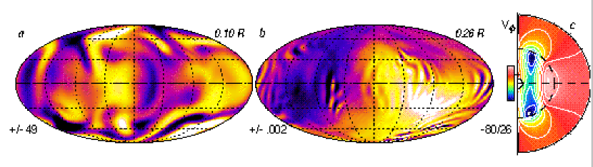
Figure 1: Flow properties of core convection in the progenitor hydrodynamic simulation case E from BBT. $(a)$ Radial velocity $v_{r}$ at one instant in mid-core (at $r=0.10R$), shown in a global view as a Mollweide projection. Broad regions of upflow are in light tones, and downflows dark, as indicated by color bar with ranges in m s^-1. $(b)$ Companion view of $v_{r}$ within surrounding radiative envelope (at $r=0.26R$), showing signature of the relatively weak internal gravity waves excited by the plumes of penetration. $(c)$ Resulting differential rotation established in the computational domain displayed in cross-section of radius and latitude. Shown as a contour plot is the time and longitudinally averaged zonal velocity $\hat{v}_{\phi}$, which possesses a central column of particularly slow rotation (retrograde relative to the frame). The equator is denoted by the dashed line, the rotation axis is vertical, and the outer extent of the prolate core is indicated by the dotted curve.

The simulations described here take as their starting points an evolved instant in the hydrodynamic simulations of core convection described in BBT. We illustrate in Figure 1 some of the striking dynamical properties revealed by one of those progenitor simulations. Figure 1$a$ shows a global mapping at one instant of the radial velocity deep within the core in case E, which is rotating at the solar rate. In this Mollweide projection, meridian lines are seen as curved arcs, and lines of constant latitude are indeed parallel. Convection within the core involves broad sweeping flows that span multiple scale heights, with little apparent asymmetry between upflows (light features) and downflows (dark tones). The convective flows in such global domains can readily plunge through the center, thus coupling widely separated sites. The flows are highly time dependent, with complex and intermittent features emerging as the simulations evolve. Such vigorous convection is able to penetrate into the overlying radiative zone, with that extent varying with latitude. The upward-directed penetrating plumes serve to excite gravity waves in the stable envelope, seen in Figure 1$b$ as localized ripples on many scales.

The coupling of convection with rotation in these spherical geometries yields a prominent differential rotation exhibited in Figure 1$c$. The mean zonal flows shown there (relative to the rotating frame) are characterized by a central cylindrical column of slow rotation. Within the bulk of the convection zone, this differential rotation is driven primarily by the Reynolds stresses associated with the convection, helped by meridional circulation and opposed by viscous stresses. Near the interface between the core and the radiative envelope, baroclinicity also plays an important role.

The penetrative convection yields a nearly adiabatically stratified core region that is prolate in shape and aligned with the rotation axis (shown by the dashed curve in Figure 1$c$). This is surrounded by a further region of overshooting in which the convective plumes can mix the chemical composition but do not appreciably modify the stable (subadiabatic) stratification. The outward extent of this zone is roughly spherical. Our progenitor simulations in BBT have thus revealed that core convection establishes angular velocity profiles with a distinctive central column of slowness, a prolate shape to the well-mixed core, and a broad spectrum of gravity waves in the radiative envelope.

3 DYNAMO ACTION REALIZED IN CORE

We have found that vigorous core convection coupled with rotation clearly admits magnetic dynamo action. The initial seed magnetic fields introduced into our two progenitor hydrodynamic simulations are amplified greatly by the convective and zonal flows, ultimately yielding magnetic fields that possess energy densities comparable to that in the convection itself. Here we begin by assessing the growth of the magnetic fields and their saturation, the morphology of the magnetism and the resulting modified convection, and the intricate time dependence of the sustained fields and flows.

3.1 Growth and Saturation of Magnetic Fields

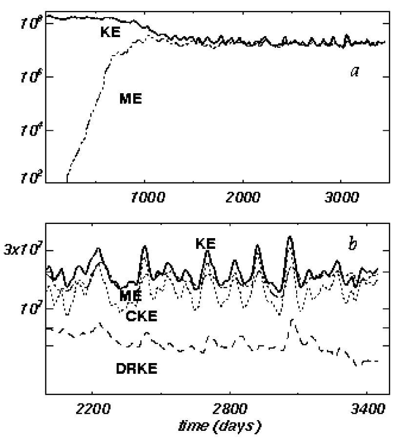
Figure 2: Temporal evolution in case C4m of the volume-averaged total kinetic energy density (KE) and the magnetic energy density (ME). ($a$) The initial seed magnetic field is amplified by many orders of magnitude. After an initial phase in which ME grows exponentially, it equilibrates to a level in which it becomes comparable to KE, which has been lessened by the feedback of the magnetism upon the flows. ($b$) Detailed view of fluctuations of energy densities once equilibration is approached, showing also energy densities of the convection (CKE) and the differential rotation (DRKE).

The temporal evolution of the magnetic energy (ME) and kinetic energy (KE) densities (volume-integrated and relative to the rotating frame) in case C4m is displayed in Figure 2$a$. The magnetic field undergoes an initial phase of exponential growth from its very weak seed field that lasts about 1000 days. In case Em (not shown), the initial phase of growth lasts about 1700 days. The seed dipole fields are in both simulations amplified by more than eight orders of magnitude. The different growth rates for the magnetic field realized in the two simulations result from the differing Reynolds numbers and magnetic diffusivities adopted. Both have magnetic Reynolds numbers (see Table 1) well in excess of the threshold values that earlier studies of convection in spherical shells (e.g., Gilman 1983; Brun et al. 2004) have found necessary for dynamo action, typically $R_{m}\approx 300$. This exponential growth is followed by a nonlinear saturation phase, during which the Lorentz forces acting upon the flows yield statistical equilibria in which induction is balanced in the large by ohmic dissipation. The magnetic field attains different saturation amplitudes in the two simulations. In case C4m, the energy density in the magnetic field (ME) is typically about $88$% of the kinetic energy density (KE), whereas in case Em it is about 28% but fluctuates considerably in several phases of behavior. Such field amplitudes are sustained for longer than the magnetic diffusion time across the computational domain – here, $\tau\sim L^{2}/(\pi^{2}\eta)\sim 3900$ days (Moffatt 1978) – implying that the magnetic field is being actively maintained against ohmic decay. Thus sustained dynamo action has probably been realized. The different set of parameters used in the two simulations appear to account for the different saturation field strengths that are realized.

The strong magnetic fields established by dynamo action within the core are expected to interact with the convective and zonal flows. A clear indication of such feedback is provided by the reduction of KE visible in Figure 2$a$ after about $1000$ days. This first becomes apparent once ME grows to about 1% of KE, as the magnetic fields begin to significantly modify the flows through the Lorentz (${\bf j}\mbox{\boldmath$\times$}{\bf B}$) term in equation (3), much as in simulations of strong dynamo activity in the solar convection zone (Brun, Miesch & Toomre 2004). The reduction in KE here is due primarily to a significant decline in the energy contained in the differential rotation (DRKE). In simulation C4m, DRKE decreases to only 3% of its value in the hydrodynamic progenitor simulation C4 (see also Table 3). In case Em, the decline is also appreciable, with DRKE dropping to 19% of its value in the hydrodynamic simulation. We consider issues of the resulting differential rotation and its linkage to temporal variations of ME in §4.1.

Like the convective and zonal flows that build and sustain them, the magnetic fields in these simulations are highly variable in time. This variability is apparent in Figure 2$b$, which shows the evolution of various energy densities over an interval subsequent to the initial exponential growth of the magnetic field. Shown are the energies in the convection (CKE) together with KE, DRKE, and ME. Though no continuous growth or decline of the energy densities is evident, they show considerable variations for this case C4m. During this interval, KE fluctuates by about a factor of three, with most of this variation reflecting that of CKE. The modulations in CKE have a temporal spacing of about 130-140 days, or roughly 20 rotation periods. Here ME likewise varies, as the convective and zonal flows serve to modify the magnetic fields through the production term in the induction equation (5). Indeed, during some intervals in the evolution of case C4m shown in Figure 2$b$, ME actually exceeds KE. It is interesting that the field strengths achieved in case C4m thus roughly represent equipartition between the flows relative to the rotating frame and the magnetism. Such values of ME represent typical rms field strengths in the core of about 67 kG, as compared to rms flow velocities that are about 30 m s^-1 (Table 2).

3.2 Morphology of Flows and Magnetism

Within the core, broad convective flows sweep through the spherical domain, with large-scale regions of upflow and downflow serving to couple widely separated regions. The global connectivity permitted in these full spheres, together with the fairly small density contrasts present, results in motions that can span large fractions of a hemisphere and extend radially through much of the convection zone.

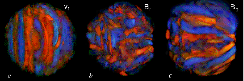
Figure 3: Volume renderings of flow and magnetic structures at one instant in case C4m near the outer boundary of the prolate convective core. ($a$) Radial velocity $v_{r}$ exhibits columnar structures aligned with the rotation axis (here oriented vertically). Little asymmetry is apparent between upflows (reddish) and downflows (bluish). ($b$) The radial magnetic field $B_{r}$ is more tangled, with field polarity shown in contrasting tones. ($c$) The longitudinal magnetic field $B_{\phi}$ possesses a distinctive ribbon-like morphology, with coherent bands that extend around much of the core.

Such global-scale convective flows are apparent in Figure 3$a$, which shows a volume rendering of a snapshot of the radial velocity $v_{r}$ near the outer boundary of the convective core in case C4m. The region of vigorous convection is slightly prolate in shape, much as in the progenitor, extending farther in radius near the poles than near the equator. No obvious asymmetry between regions of upflow and downflow is visible. This stands in sharp contrast to the results of solar convection simulations that exhibit broad upflows together with narrow and fast downflows.

The magnetic fields sustained within the convection zone are characterized by smaller scale features than are present in the convective flows. The intricate nature of the field is most apparent in Figure 3$b$, which shows the radial component of magnetic field $B_{r}$. Here the field appears as a tangled collection of positive and negative polarity on many different scales. The finer structure present in the magnetic fields than in the convective flows comes about partly because we have taken the magnetic diffusivity to be smaller than the viscous diffusivity (with $P_{m}=5$).

The longitudinal fields $B_{\phi}$ shown in Figure 3$c$ likewise possess small-scale structure, but also exhibit organized bands of magnetism that wrap around much of the core. These broad ribbons of toroidal field may arise due to stretching by gradients of angular velocity near the interface between the core and the radiative envelope. Such stretching and amplification of toroidal field by differential rotation, described in mean-field theories as the $\omega$-effect, mirrors what is thought to occur in the tachocline of rotational shear at the base of the solar convection zone. In the sun, magnetic fields are thought to be pumped downward from the envelope convection zone into the radiative interior, with the tachocline at the interface producing strong toroidal fields that eventually rise by magnetic buoyancy through the convection zone (e.g., Charbonneau & MacGregor 1997). Here we may be seeing the reverse analog of such a process in stars with convective interiors surrounded by radiative envelopes.

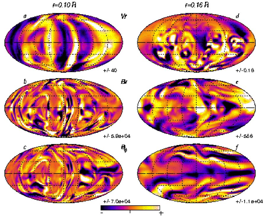
Figure 4: Global mappings at one instant in case Em of $v_{r}$, $B_{r}$, and $B_{\phi}$ sampled on two spherical surfaces, both at mid-core ($r=0.10R$, left) and in region of penetration and overshooting ($r=0.16R$, right). Shown are Mollweide projections with the dashed horizontal line denoting the equator. All fields share the same symmetric color table, with positive values in bright tones and negative ones in dark tones. The amplitude ranges are indicated adjacent to each panel, with magnetic fields in G and velocities in m s^-1.

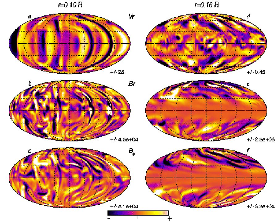
Figure 5: As in Fig. 4, global Mollweide projections of $v_{r}$, $B_{r}$, and $B_{\phi}$ for the more rapidly rotating case C4m at one instant in time.

The intricate networks of magnetic fields and convective flows are also revealed in Figure 4 (for case Em) and in Figure 5 (for case C4m) by global mappings of the radial velocity ($v_{r}$) together with the radial ($B_{r}$) and azimuthal ($B_{\phi}$) magnetic fields at two depths. Deep within the convective core (at $r=0.10R$, right), the finely threaded magnetic field coexists with the relatively broad patchwork of convective flows. Features in $v_{r}$ and $B_{r}$ possess evident links, with the convective downflow lanes containing strong radial magnetic field of both polarities. In contrast, upflows contain few strong magnetic structures. The azimuthal field $B_{\phi}$ within the core appears to be quite patchy, with little correlation to the radial velocity field $v_{r}$. Finer structure is present in all the fields displayed for case C4m (Fig. 5), relative to case Em, owing mostly to the slightly smaller viscosities and resistivities adopted for C4m.

Near the boundary of the convective core and the radiative envelope ($r=0.16R$, left), $v_{r}$ and $B_{r}$ both possess considerably smaller amplitudes than in the deep interior, with $v_{r}$ in case Em (Fig. 4) lessened by a factor of 240 and $B_{r}$ by a factor of 100. This suggests that the spherical surface shown cuts through a region where only weak overshooting of the convection survives. In case C4m (Fig. 5$a$,$b$), the amplitudes of $v_{r}$ and $B_{r}$ are reduced by smaller factors (of 64 and 18 respectively) in going from $r=0.10R$ to $r=0.16R$, most likely because one is sampling here the penetrative convection more directly, probably because of the weaker stable stratification in this case. In contrast, $B_{\phi}$ near the core boundary in both cases is only slightly diminished from its interior strength, and may reflect the continuing production of toroidal field there by rotational shear. The overall magnetic fields at the core boundary are of larger physical scale than the fields deeper down, and $B_{\phi}$ (Figs. 4$c$, 5$c$) shows the same broad and wavy, ribbon-like features evident in the volume renderings of Figure 3$c$. In case C4m (Fig. 5$c$), the magnetic field at this radius ($r=0.16R$) is much stronger at high latitudes than at the equator, reflecting the prolate shape of the strongly magnetized core of convection. The spherical surface viewed here lies inside this prolate region near the poles, but outside it at the equator. Thus the stronger influence of rotation in this case C4m has yielded greater departures from a spherical shape for the core with penetration than is realized in case Em, helped also by the reduced stiffness of the radiative envelope in case C4m.

Our global mappings (at $r=0.16R$) also reveal that the pummelling of the base of the radiative envelope by the upward-directed convective plumes serves to excite a broad range of internal gravity waves. These waves are visible at the low latitudes in Figures 4$a$, 5$a$ as low-amplitude ripples of small physical scales. Similar gravity waves were seen in the progenitor non-magnetic simulations in BBT.

3.3 Time-Dependence of Sustained Flows and Fields

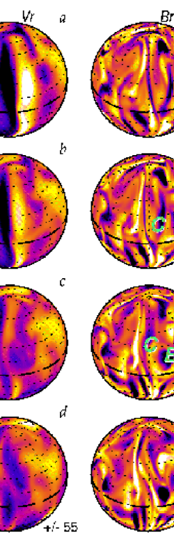
Figure 6: Rapid sampling in time of the evolution of structures seen in $v_{r}$ (left) and $B_{r}$ (right), as viewed on spherical surfaces at mid-core ($r=0.10R$) for case Em. The four snapshots are separated by 6 days each, starting from a mature time $t_{o}$ within the simulation. Features (A, B, C, labeled) in the flows and magnetism persist, but are advected and sheared, propagate relative to the frame, and can cleave into smaller structures. The color table is as in Fig. 4, and scaling is indicated.

The convective flows and the magnetic fields that they generate in our two cases evolve in a complicated fashion. Throughout the convective core, we have observed the birth of magnetic structures, their advection and shearing by the flows, and their mergers with other features or cleaving into separate structures. Some flows and magnetic structures persist for many days, while others rapidly fade away. A brief sampling of such behavior in case Em is provided in Figure 6 showing a succession of spherical views of both $v_{r}$ and $B_{r}$ in mid-core ($r=0.10R$) at four closely spaced snapshots (each 6 days apart). Several features amidst the magnetism, labeled $A$, $B$, $C$ in Figure 6, propagate in a slightly retrograde fashion (to the left) over the interval sampled. Features $A$ and $B$ remain confined to low latitudes, with feature $B$ varying considerably in strength and size as the simulation evolves. In Figure 6$e$, this structure is visible as a weak patch of negative $B_{r}$ at a latitude of about 20°; later it has become a much broader feature of greater amplitude (Fig. 6$h$), seen as a dark patch at a latitude of about 15°. Feature $C$, which at first appears as a narrow structure of negative polarity spanning latitudes from the equator to about 45°, then propagates toward higher latitudes, and is sheared and weakened. The convective flows exhibit similar changes, with a coherent downflow lane (Fig. 6$a$) spanning both hemispheres gradually breaking up into multiple structures.

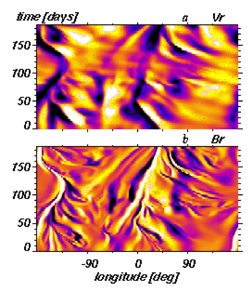
Figure 7: Extended evolution and propagation assessed by time-longitude sampling of ($a$) $v_{r}$ and ($b$) $B_{r}$ at mid-core ($r=0.10R$) in case Em at the equator. At such low latitudes, persistent features in both $v_{r}$ and $B_{r}$ tend to propagate prograde (to the right) in longitude (relative to the frame). There is close correspondence in the structures evident in $v_{r}$ and $B_{r}$. The color table and scaling is shared with Fig. 6, as is the sampling starting time $t_{o}$.

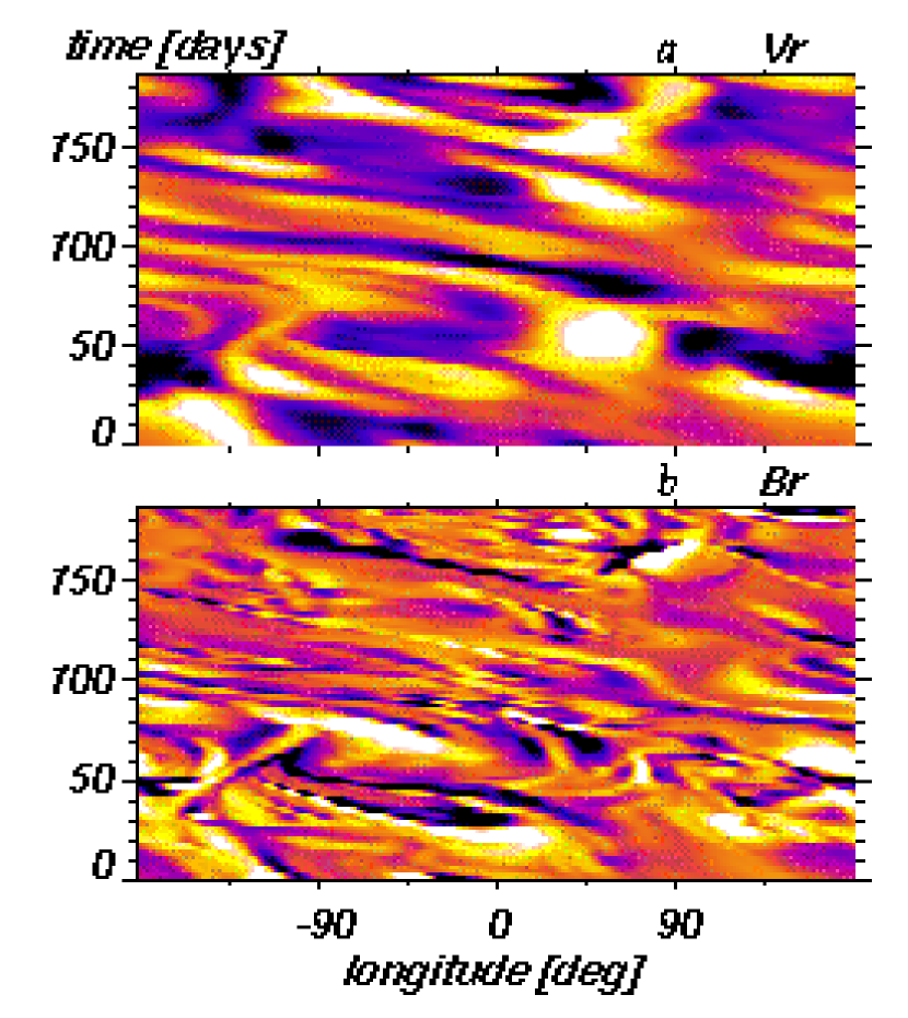
Figure 8: As in Fig. 7, but time-longitude maps for $v_{r}$ and $B_{r}$ at latitude 60°. Here the propagation of features in both fields is distinctly retrograde relative to the frame.

Such rich time dependence is assessed over longer temporal intervals in case Em by turning to time-longitude mappings in Figures 7 and 8. These show the variation with time of $v_{r}$ and $B_{r}$ sampled (at $r=0.10R$) for all longitudes either at the equator (Fig. 7) or at 60$\arcdeg$ latitude (Fig. 8). Coherent downflow lanes are visible in these time-longitude mappings of $v_{r}$ as dark bands tilted to the right, indicating prograde propagation (relative to the frame), or to the left or retrograde, which often persist for multiple rotation periods. Similar evolution is observed in the companion mappings of $B_{r}$, with most major structures evident in both the flows and the magnetism. Much as in Figure 4, the persistent convective downflows contain magnetic fields of mixed polarities, whereas the upflows are largely devoid of strong magnetic structures. The propagation of these large-scale structures tends to be prograde at the equator (Fig. 7) and strongly retrograde at high latitudes (Fig 8). There is also substantial evolution of the flows on short time scales, with some striking features of the convection rapidly emerging and then fading. Similarly, the magnetic field exhibits both rapid evolution of some structures, and others that survive for extended periods of time. Identification of persistent features amidst the magnetism is occasionally made more difficult by the finely threaded field topology. However, structures evident in $B_{r}$ generally appear to be advected and to propagate in roughly the same fashion as features in $v_{r}$, with both tending to wax and wane as the simulations evolve.

4 MEAN FLOWS AND TRANSPORT

In the deep spherical domains studied here, the Coriolis forces associated with rotation can have major impacts on the structure of the convective flows and thus on the manner in which they redistribute angular momentum. When that influence is strong, as when the convective overturning time is at least as long as the rotation period (with the convective Rossby number $R_{c}$ of order unity or smaller), a strong differential rotation may be achieved and maintained. This was realized in all the cases studied in BBT. The dynamo action and consequent intense magnetic fields realized in our current simulations must feed back strongly on the convection through the Lorentz forces, probably reducing the differential rotation that can be maintained. Intuitively, one expects that the presence of magnetic fields will tend to diminish the differential rotation, with the field lines that thread the core acting like rubber bands to couple disparate regions and enforce more uniform rotation. Such an analogy is too simple given the tangled and intermittent nature of the magnetic fields in our simulations, yet the expectation that the presence of magnetism leads to reduced differential rotation turns out to be largely correct. We now consider the mean zonal flows of differential rotation that are realized in our cases Em and C4m, their variations in time, and the manner in which they are sustained.

4.1 Nature of Accompanying Differential Rotation

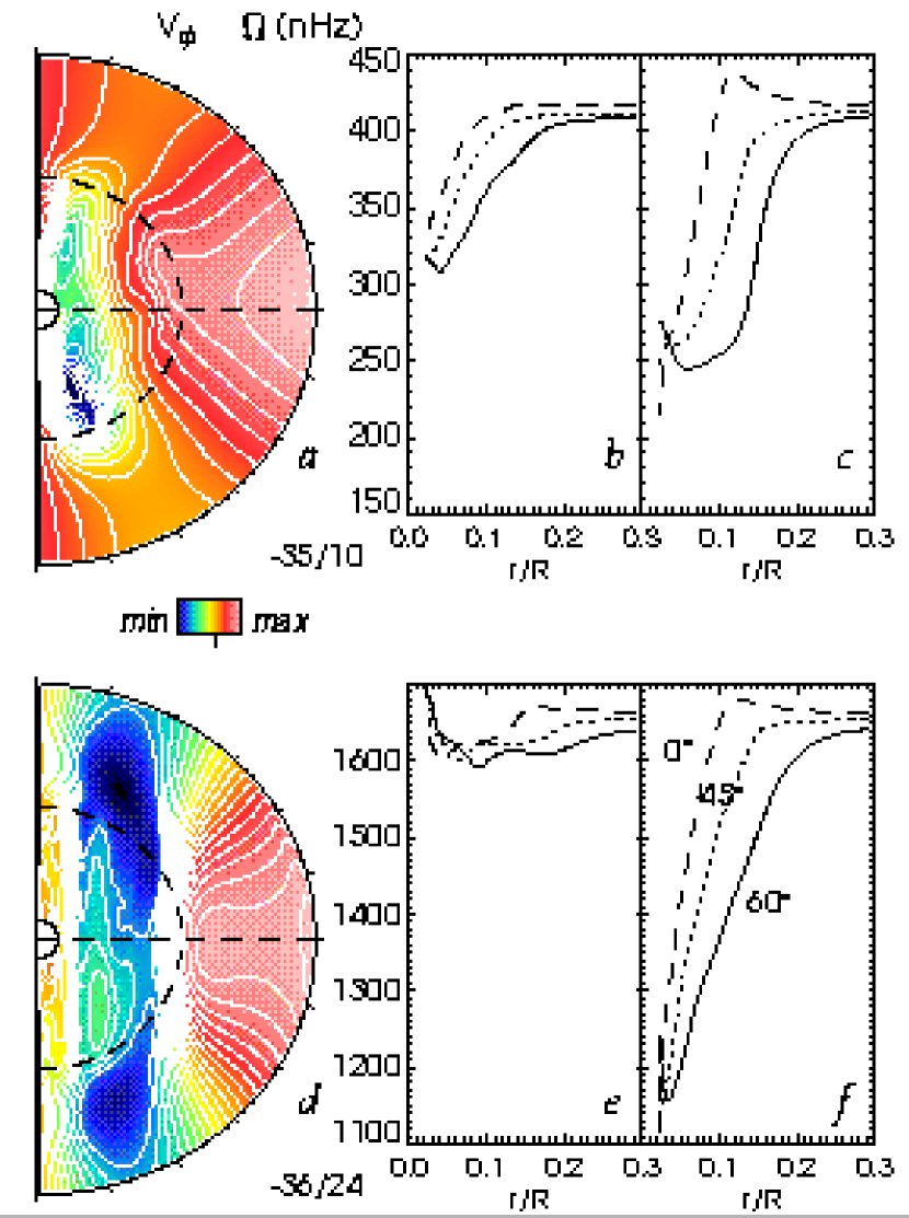
Figure 9: Differential rotation established in case Em (top) and C4m (bottom), and their progenitors. ($a$,$d$) Mean zonal velocity $\hat{v}_{\phi}$, averaged in time and longitude, as contour plots in radius and latitude, with color bar and ranges (in m s^-1) indicated. Equator is horizontal, rotation axis is vertical, and outer extent of convective core is indicated by dashed curve. ($b$,$e$) Angular velocity $\hat{\Omega}$ with radius for latitudinal cuts at 0°,45°, and 60°. ($c$,$f$) $\hat{\Omega}$ achieved in progenitor nonmagnetic models. The magnetism acts to inhibit the strong angular velocity contrasts realized in the progenitor simulations.

The differential rotation profiles achieved in our two cases Em and C4m are shown in Figure 9. These are displayed first as contour plots with radius and latitude of the longitudinal (or zonal) velocity $\hat{v}_{\phi}$, with the hat denoting an average in time and longitude. Shown also are plots of the radial variation of the associated angular velocity $\hat{\Omega}$ along three latitudinal cuts, contrasting the behavior in our magnetic simulations with that of their progenitors. The latter emphasize that in case Em the angular velocity contrasts have been lessened almost twofold from the hydrodynamic progenitor. In case C4m that contrast has been nearly eliminated. The contours of $\hat{v}_{\phi}$ emphasize that central columns of slow rotation are realized in both cases, as in their progenitors, but with reduced zonal flow amplitudes (see Fig. 1$c$). Both $\hat{v}_{\phi}$ profiles exhibit some asymmetry between the northern and southern hemisphere, with such behavior more pronounced for case Em (Fig. 9$a$). Noteworthy for case C4m is that the column of slowness in $\hat{v}_{\phi}$ extends well into the radiative envelope, owing in part to the stronger meridional circulations exterior to the core achieved with the faster frame rotation. The longitudinal velocity in C4m appears to be nearly constant on cylinders aligned with the rotation axis, somewhat akin to Taylor-Proudman columns achieved when rotational constraints are strong.

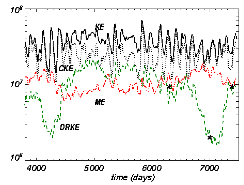
Figure 10: Detailed view in case Em of variations in the volume-averaged energy densities of the convection (CKE), differential rotation (DRKE), total kinetic energy density (KE), and magnetic energy (ME). Here DRKE undergoes two pronounced minima, the beginnings of which coincide with times at which ME climbs above $\sim 1.2\times 10^{7}$ erg cm^-3, or about 40% of KE. Indicated on the DRKE trace are the three times sampled for the differential rotation snapshots in Fig. 11.

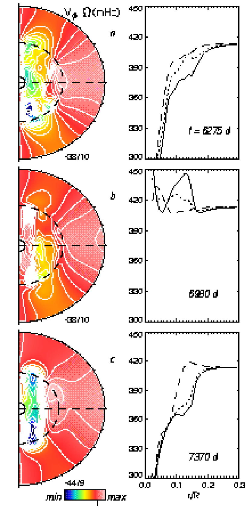
Figure 11: Differential rotation achieved in case Em at three different time sampling intervals before ($a$, upper), during ($b$, middle), and after ($c$, lower) a grand minimum in DRKE in Fig. 10. Shown as contour plots (left) are the longitudinal averaged zonal velocity $\hat{v}_{\phi}$ averaged over brief (20 day) intervals, accompanied by (right) angular velocity $\hat{\Omega}$ as radial cuts at the three latitudes indicated.

With the temporal changes seen in our convective flows and magnetism (Fig. 6) come also substantial variations in the differential rotation that they establish. This is most pronounced in case Em. Figure 10 shows a detailed view of temporal fluctuations in volume-averaged energy densities of the differential rotation (DRKE), convection (CKE), and magnetism (ME). These reveal that during extended intervals DRKE exceeds ME, but with moderate oscillations; such an interval was sampled in producing Figure 9. The fairly regular accompanying oscillations in CKE (and thus also KE) have periods of about 150-200 days, as contrasted to the rotation period of 28 days. There are also remarkable brief intervals during which DRKE plummets by nearly an order of magnitude, with two such shown in Figure 10 at about 4200 days and 7000 days in the simulation. The onset of those grand minima in DRKE coincide with times when ME has climbed to values greater than about 40% of KE. This suggests that strengthening magnetic fields can lead to abrupt collapses in the differential rotation established by the convection, followed by a recovery. This arises partly from the strong feedback of the Lorentz forces on the convection and on the differential rotation, both of which serve to build the fields through induction. With the consequent diminished flows, the field production is lessened, and so the magnetic fields weaken. Once below a given threshold (here ME less than 40% of KE), the convection regains its strength, leading to stronger Reynolds stresses (see §4.2) that reestablish the differential rotation, with magnetic induction once again invigorated. Thus the cycle lasting about 2000 days begins anew. Such intricate behavior seen in case Em is not realized in case C4m where ME and KE are always comparable though moderately variable (see Fig. 2$b$). Since ME in this case is far stronger, a cyclic behavior in which the Lorentz forces oscillate between being strong or weak is not realized. The complex changes in the differential rotation achieved in case Em are shown in Figure 11 that samples three short temporal averages of $\hat{v}_{\phi}$ and $\hat{\Omega}$. These examine intervals prior, during, and after the second pronounced minimum of DRKE (Fig. 10). During that minimum the angular velocity contrast within the core (Fig. 11$b$) is modest, and the retrograde column of slowness in $\hat{v}_{\phi}$ is barely there. The samples before (Fig. 11$a$) and after (Fig. 11$c$) show zonal flows and angular velocity contrasts much as in Figures 9$a$,$b$, possessing central regions of slow rotation. In contrast, no comparable large variation in zonal flows are realized in case C4m, where angular velocity contrasts are modest at all times, much as in the long time average shown in Figure 9$d$,$e$.

4.2 Redistributing the Angular Momentum

The complex MHD systems studied here exhibit a rich variety of responses, with intricate time dependence seen in both the flows and magnetic fields. How the zonal flows seen as differential rotation arise and are sustained, how they interact with the magnetism, and how they vary in time are thus all sensitive matters. This behavior cannot now be predicted from first principles, but the present simulations offer a unique opportunity to determine the roles played by different agents in transporting angular momentum and giving rise to the differential rotation. Since our case Em exhibits strong angular velocity contrasts, albeit variable, we will here examine how these are established.

Our simulations were conducted with stress-free and purely radial magnetic field boundary conditions, so no net external torque is applied to the computational domain. Thus total angular momentum within the simulations is conserved. We can assess the transport of angular momentum within these systems in the manner of Brun, Miesch & Toomre (2004) (see also Elliott, Miesch, & Toomre 2000). We consider the $\phi$-component of the momentum equation expressed in conservative form and averaged in time and longitude:

$$\frac{1}{r^{2}}\frac{\partial(r^{2}{\cal F}_{r})}{\partial r}+\frac{1}{r\sin\theta}\frac{\partial(\sin\theta{\cal F}_{\theta})}{\partial\theta}=0,$$ (11)

involving the mean radial angular momentum flux

$${\cal F}_{r}=\bar{\rho}r\sin\theta[-\nu r\frac{\partial}{\partial r}\left(\frac{\hat{v}_{\phi}}{r}\right)+\widehat{v_{r}^{{}^{\prime}}v_{\phi}^{{}^{\prime}}}+\hat{v}_{r}(\hat{v}_{\phi}+\Omega r\sin\theta)-\frac{1}{4\pi\bar{\rho}}\widehat{B_{r}^{{}^{\prime}}B_{\phi}^{{}^{\prime}}}-\frac{1}{4\pi\bar{\rho}}\hat{B}_{r}\hat{B}_{\phi}]$$ (12)

and the mean latitudinal angular momentum flux

$${\cal F}_{\theta}=\bar{\rho}r\sin\theta[-\nu\frac{\sin\theta}{r}\frac{\partial}{\partial\theta}\left(\frac{\hat{v}_{\phi}}{\sin\theta}\right)+\widehat{v_{\theta}^{{}^{\prime}}v_{\phi}^{{}^{\prime}}}+\hat{v}_{\theta}(\hat{v}_{\phi}+\Omega r\sin\theta)-\frac{1}{4\pi\bar{\rho}}\widehat{B_{\theta}^{{}^{\prime}}B_{\phi}^{{}^{\prime}}}-\frac{1}{4\pi\bar{\rho}}\hat{B}_{\theta}\hat{B}_{\phi}].$$ (13)

In the above expressions, the terms on both right-hand-sides denote contributions respectively from viscous diffusion (which we denote as ${\cal F}_{r}^{VD}$ and ${\cal F}_{\theta}^{VD}$), Reynolds stresses (${\cal F}_{r}^{RS}$ and ${\cal F}_{\theta}^{RS}$), meridional circulation (${\cal F}_{r}^{MC}$ and ${\cal F}_{\theta}^{MC}$), Maxwell stresses (${\cal F}_{r}^{MS}$ and ${\cal F}_{\theta}^{MS}$) and large-scale magnetic torques (${\cal F}_{r}^{MT}$ and ${\cal F}_{\theta}^{MT}$). The Reynolds stresses are associated with correlations of the fluctuating velocity components (shown primed) that arise from organized tilts within the convective structures. Similarly, the Maxwell stresses are associated with correlations of the fluctuating magnetic field components that arise from tilt and twist within the magnetic structures.

Analyzing the components of ${\cal F}_{r}$ and ${\cal F}_{\theta}$ is aided by integrating over co-latitude and radius to deduce the net fluxes through shells at various radii and through cones at various latitudes, such that

$$I_{r}(r)=\int_{0}^{\pi}{\cal F}_{r}(r,\theta)\,r^{2}\sin\theta\,d\theta\;\mbox{ , }\;I_{\theta}(\theta)=\int_{r_{bot}}^{r_{top}}{\cal F}_{\theta}(r,\theta)\,r\sin\theta\,dr\,.$$ (14)

We then identify in turn the contributions from viscous diffusion (VD), Reynolds stresses (RS), meridional circulation (MC), Maxwell stresses (MS) and large-scale magnetic torques (MT). This helps to assess the sense and amplitude of angular momentum transport within the convective core and the radiative exterior by each component of ${\cal F}_{r}$ and ${\cal F}_{\theta}$. We now examine the transports achieved within case Em by temporally averaging the fluxes over the interval spanning from 6700 to 7000 days, during which the system was undergoing changes (see Fig. 10).

Turning first to the integrated radial fluxes of angular momentum in Figure 12$a$, we see that the Maxwell stresses ($I_{r}^{MS}$) are playing a major role in the radial transport, acting in the outer portions of the core to transport angular momentum radially outwards, and deeper down to transport it inwards. In this they are opposed principally by meridional circulations ($I_{r}^{MC}$), and aided by the Reynolds stresses ($I_{r}^{RS}$) associated with the convective flows. The strong Maxwell stresses realized in our simulations are noteworthy, for they lead here to major departures from the angular momentum balance that was achieved in the progenitor hydrodynamic models. Over the evolution interval for case Em sampled in Figure 12$a$, the Maxwell stresses act in concert with the Reynolds stresses throughout much of the core, even though the corresponding terms in equation (12) carry opposite signs. This indicates that correlations between the radial and longitudinal components of the fluctuating magnetic field are reversed with respect to those of the fluctuating velocity field. Such behavior was not realized in the solar convection simulations of Brun et al. (2004), and is less pronounced in our companion case C4m. We also see that the torques provided by the axisymmetric magnetic fields ($I_{r}^{MT}$) are small throughout most of the convective core, in keeping with the finding in §6 that the mean axisymmetric fields are dwarfed in strength by the fluctuating ones. However, near the outer boundary of the core these mean magnetic torques grow more significant, in keeping with the mean fields there becoming a significant contributor to the magnetic energy. There they act together with the Maxwell and Reynolds stresses to transport angular momentum outwards. The viscous flux is everywhere negative and fairly small relative to the other components. All of the component fluxes decrease rapidly outside of the convective core, as both convective motions and magnetic fields vanish.

The net radial flux $I_{r}$ (Fig. 12$a$) would be zero in a steady state but here is markedly negative. However, since in case Em the differential rotation shows prominent changes with time, there must be non-zero net fluxes of angular momentum to accomplish such changes. Over the interval sampled by Figure 12, the system is transitioning from a state of high DRKE – characterized by a strongly retrograde core – to one of low DRKE with only small angular velocity contrasts (see Fig. 10). Thus the central regions of the convective core are being spun up, and so there must be a net angular momentum flux inward. Figure 12$a$ confirms that this is indeed occurring during this interval.

The integrated latitudinal angular momentum fluxes in Figure 12$b$ also reveal a complex interplay among the different transport mechanisms. Here the Maxwell stresses ($I_{\theta}^{MS}$) act largely to slow down the equator (by transporting angular momentum toward the poles), opposing the strong Reynolds stresses ($I_{\theta}^{RS}$) that seek to accelerate it. Thus, in contrast to the radial integrated fluxes, the Reynolds and Maxwell stresses transport angular momentum in opposite directions. Similar results for the respective role of the Reynolds and Maxwell stresses in tranporting angular momentum latitudinally are found in the solar magnetic cases computed by Brun et al. (2004). Meridional circulations ($I_{\theta}^{MC}$) also generally act to accelerate the equator, though the complicated multi-celled nature of those circulations makes the angular momentum flux they provide decidedly nonuniform. The weak axisymmetric magnetic torques ($I_{\theta}^{MT}$), like their strong fluctuating counterparts the Maxwell stresses, act to oppose the equatorial acceleration afforded by the Reynolds stresses. Viscous diffusion plays only a small role, but also tends to transport angular momentum away from the equator.

Although Figure 12 assesses the angular momentum transports during an interesting interval marked by changes in the differential rotation, the character of the various contributing fluxes is much the same during other intervals. Examining these fluxes provides clues as to why the magnetic simulations exhibit much weaker differential rotation (or DRKE) than their progenitors. Whereas in the progenitor the Reynolds stresses $I_{\theta}^{RS}$ that sought to accelerate the equator competed only against meridional circulations and viscous diffusion, here they must also counteract the poleward transport of angular momentum provided by the Maxwell stresses and large-scale magnetic torques (Fig. 12$b$). Though in principle the fluxes due to the Reynolds stresses and meridional circulations could adjust to compensate for such poleward transport, this was not realized in case Em. Thus the speeding up of the equatorial regions of the outer core was lessened, and so too the slowing down of the central column, with an overall decrease in the angular velocity contrast.

4.3 Radial Transport of Energy

Since convection in the core arises because of the need to move energy radially outward, we now assess the role of different agents in transporting the energy within our simulations. Figure 13 presents the radial energy fluxes provided by various physical processes, converted to luminosities and normalized to the stellar luminosity. The total luminosity $L(r)$ and its components are defined by

$$F_{e}+F_{k}+F_{\rm r}+F_{u}+F_{v}+F_{m}=\frac{L(r)}{4\pi r^{2}},$$ (15)

with

$$F_{e} = \bar{\rho}\,c_{p}\,\overline{v_{r}T^{\prime}}\,,$$ (16)

$$F_{k} = \frac{1}{2}\,\bar{\rho}\,\overline{v^{2}v_{r}}\,,$$ (17)

$$F_{r} = -\kappa_{r}\,\bar{\rho}\,c_{p}\,\frac{d\bar{T}}{dr}\,,$$ (18)

$$F_{u} = -\kappa\,\bar{\rho}\,\bar{T}\,\frac{d\bar{S}}{dr}\,,$$ (19)

$$F_{v} = -\overline{{\bf v}\cdot{\bf\cal D}}\,,$$ (20)

$$F_{m} = \frac{c}{4\pi}\,\overline{E_{\theta}B_{\phi}-E_{\phi}B_{\theta}}\,,$$ (21)

where the overbar denotes an average over spherical surfaces and in time, ${\bf E}=4\pi\eta{\bf j}c^{-2}-({\bf v}\times{\bf B})c^{-1}$ is the electric field, $F_{e}$ the enthalpy flux, $F_{k}$ the kinetic energy flux, $F_{\rm r}$ the radiative flux, $F_{u}$ the unresolved eddy flux, $F_{v}$ the viscous flux and $F_{m}$ the Poynting flux. The unresolved eddy flux $F_{u}$ is the enthalpy (heat) flux due to subgrid-scale motions, which in our LES-SGS approach takes the form of a thermal diffusion operating on the mean entropy gradient. The kinetic energy flux, the viscous flux, the Poynting flux and the flux carried by unresolved motions are here all small compared to $F_{e}$ and $F_{r}$.

The balance of energy transport is much as in our progenitor models in BBT. As shown in Figure 13, within case C4m the enthalpy flux is maximized near the middle of the convective core (at $r=0.08R$), where it serves to carry about 50% of the stellar luminosity, with the remainder being transported by radiation. Within the nearly adiabatic stratification established in the convective core (with $\nabla-\nabla_{ad}\sim 10^{-7}$), the associated temperature gradient serves to specify a radiative flux $F_{r}$ that increases steadily with radius. Thus $F_{e}$ is forced to decrease in the outer half of the unstable core. Beyond the boundary of the convective core, the enthalpy flux becomes negative, owing to the anti-correlation of radial velocity and temperature fluctuations as penetrative motions are braked. This inward directed enthalpy flux is also manifested as a small dip in the total luminosity in Figure 13. In real stars, or in fully relaxed simulations, the radiative flux in that region would compensate for the negative enthalpy flux. However, our simulations have not been evolved for a sufficiently long time to allow such adjustment to occur fully, since the relevant thermal relaxation time is very much longer than other dynamical timescales. The small amplitude of the Poynting flux $F_{m}$ suggests that although magnetic processes significantly impact the dynamics, they do not actively transport enough energy to modify the radial energy flux balance within the core.

5 THE MANY SCALES OF FLOWS AND FIELDS

The complex operation of the dynamo within the convective core generates magnetic fields over a broad range of spatial scales, as evident in Figures 4 and 5. The manner in which the energy in the fields and flows is distributed among these spatial scales, and between axisymmetric and fluctuating components, provides perspectives on the complicated nature of the magnetism. Thus in addition to examining the breakdown of these fields into their poloidal and toroidal components, we also examine their spectral distributions and their probability density functions.

5.1 Mean and Fluctuating Magnetic Energy

The strong magnetism generated in these simulations consists of both mean (axisymmetric) and fluctuating fields. We assess the balance between these fluctuating and mean fields, defining various components of the magnetic energy as

MTE $$= \frac{1}{8\pi}\left<B_{\phi}\right>^{2}\,,$$ (22)

MPE $$= \frac{1}{8\pi}\left(\left<B_{r}\right>^{2}+\left<B_{\theta}\right>^{2}\right)\,,$$ (23)

FTE $$= \frac{1}{8\pi}\left((B_{\phi}-\left<B_{\phi}\right>)^{2}\right)\,,$$ (24)

FPE $$= \frac{1}{8\pi}\left((B_{r}-\left<B_{r}\right>)^{2}+(B_{\theta}-\left<B_{\theta}\right>)^{2}\right)\,,$$ (25)

FME $$= \frac{1}{8\pi}\left((B_{r}-\left<B_{r}\right>)^{2}+(B_{\theta}-\left<B_{\theta}\right>)^{2}+(B_{\phi}-\left<B_{\phi}\right>)^{2}\right)\,,$$ (26)

where we recall that the angle brackets $\left<~{}\right>$ denote a longitudinal average. Here MTE denotes the energy in the mean toroidal magnetic field, MPE likewise that in the mean poloidal field, FTE the energy in the fluctuating toroidal component, FPE that in the fluctuating poloidal field, and FME the total energy in the fluctuating magnetic fields. In Figure 14, we illustrate for case Em how these components (further averaged in latitude) vary in strength with radius throughout the convective core and the surrounding radiative envelope. The ME, TME, and PME are there averaged over a temporal interval of about 100 days representative of the extended plateau of high DRKE in Figure 10.

The field within the core is mostly non-axisymmetric, with that fluctuating field energy FME accounting for about 95% of the total ME at most radii within the convective core. The remaining 5% is distributed between the toroidal and poloidal mean fields, with the former stronger there by about a factor of two (Table 3). The FME is in contrast divided in roughly equal measure between FTE and FPE (not shown). The balance of magnetic field components changes rapidly near the edge of the radiative envelope (at about $r=0.16R$). Throughout the region of overshooting, the toroidal mean field becomes a steadily larger fraction of ME, whereas the fluctuating field FME declines in proportional strength. By $r=0.185R$, TME has become as large as FME, and exterior to that radius it is the dominant contributor to the magnetism. The $m=0$ toroidal field energy MTE also remains much larger than MPE through the region of overshooting and the radiative envelope.

5.2 Spectral Distributions of Flows and Magnetism

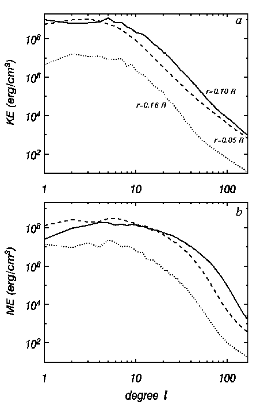
Figure 15: Time-averaged spectral distributions of ($a$) kinetic energy (KE) and ($b$) magnetic energy (ME) with degree $\ell$ for case Em, evaluated on three spheres with radii indicated.

The velocity and magnetic fields examined in Figures 4 and 5 for cases Em and C4m suggest that the magnetic field posesses relatively more small-scale structure than the flows. This is verified in Figure 15 where we display for case Em the magnetic and kinetic energy spectra computed at two depths in the convective core and within the region of overshooting. The slope of the magnetic energy spectrum (Fig. 15$b$) with degree $\ell$ is much shallower than the kinetic energy spectrum (Fig. 15$a$) and generally peaks at wavenumbers slightly higher. This means that the magnetic energy equals or exceeds the kinetic energy at both intermediate and small scales ($\ell\gtrsim 20$), even though when integrated over the volume the magnetic energy is smaller than the kinetic energy. Given that our magnetic Prandtl number is greater than unity, such behavior is expected in the range of wavenumbers located between the viscous and ohmic dissipation scales, which here are in the range $\ell>100$. More surprising is that the magnetic energy also exceeds the kinetic energy over a wide range of larger scales. Possibly some guidance is afforded by Grappin et al. (1983) in studying homogeneous isotropic MHD turbulent flows in which there was overall equipartition between ME and KE. They reported that the difference between magnetic and kinetic energy spectra should scale as $\ell^{-2}$ in the inertial range of the spectra, indicating a dominant role of the magnetic field over the flow at small $\ell$’s. This $\ell^{-2}$ scaling is not realized in our two cases here (except over a small range of degrees in the overshooting layer), perhaps owing to the effects of rotation and stratification not included in the Grappin et al. (1983) analysis. Throughout most of the convective core, both spectra have broad plateaus at low wavenumbers, with shallow peaks near $\ell=5$. For degrees $\ell\gtrsim 10$, the spectra suggest some power law behavior, but it extends only over a decade in degree so these simulations do not possess an extended inertial range. The slope of the kinetic energy spectrum (between $\ell^{-3}$ and $\ell^{-4}$) is substantially steeper than that expected for homogeneous, isotropic, incompressible turbulence, either with magnetic fields ($l^{-3/2}$) or without ($l^{-5/3}$) (e.g., Biskamp 1993). The shallower magnetic energy spectra are somewhat closer to the $\ell^{-3/2}$ behavior.

The energy contained in the dipolar and quadrupolar magnetic fields (i.e., modes $\ell=$1 and 2) is small when compared to the energy contained in all the other modes. In case Em we find that they constitute about 5% of the total magnetic energy in the core, but contribute proportionately as much as 15% in the overshooting region. The quadrupolar field is generally stronger than the dipolar one in the convective core by about a factor of 2 to 3, but in the region of overshooting the dipole term comes to dominate the quadrupole one.

In considering the energy spectra for KE and ME as a function of azimuthal wavenumber $m$ (not shown), within the convective core the dominant wavenumbers between 1 and 7 contain more power than the axisymmetric mode $m=0$, confirming the predominantly non-axisymmetric nature of both the magnetic and velocity fields. Over the same temporal interval sampled by Fig. 15, the axisymmetric $m=0$ represents about 3% of the magnetic energy at $r=0.10R$ and 5.5% at $r=0.05R$. We find similar but slightly smaller percentages in case C4m. In the radiative zone, the axisymmetric mode becomes dominant for the toroidal field and contributes about 29% to the magnetic energy contained in that layer.

5.3 Probability Density Functions

The turbulent convective flows and magnetic fields in our simulations can be further characterized by their probability density functions (pdfs). In idealized isotropic, homogeneous turbulence the velocity fields possess Gaussian pdfs, yet departures from Gaussian statistics are known to be present in many real turbulent flows. In particular, velocity differences and derivatives generally have non-Gaussian pdfs that are often described by stretched exponentials $\exp[-\beta]$ with $0.5\leq\beta\leq 2$ (e.g., Castaing, Gagne & Hopfinger 1990; Vincent & Meneguzzi 1991). The tails of the distributions are often nearly exponential ($\beta\approx 1$) but can be even flatter, particularly in the viscous dissipation range. Further, a flat slope ($\beta<2$) indicates an excess of high-amplitude events relative to a Gaussian distribution, a consequence of spatial intermittency in the flow that may be associated with the presence of coherent structures (e.g., Vincent & Meneguzzi 1991; Lamballais, Lesieur & Métais 1997).

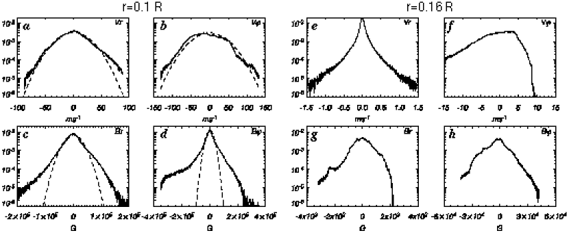
Figure 16: Time-averaged PDFs for case Em of velocities ($v_{r}$ and $v_{\phi}$) and magnetic fields ($B_{r}$, $B_{\phi}$) sampled on two spherical surfaces ($r=0.10R$ and $r=0.16R$). Some Gaussian fits to the distributions are indicated by dashed curves.

Figure 16 shows pdfs for the radial and longitudinal components of the velocity and magnetic fields for case Em on a spherical surface within the convective core ($r=0.10R$) and the region of overshooting ($r=0.16R$). The pdfs have been averaged over a 50 day interval. In the convective core, the radial and longitudinal velocities are nearly Gaussian with departure toward an exponential distribution in their wings. By contrast, both components of the magnetic fields possess strong departures from a Gaussian distribution, with pdfs closer to an exponential distribution. In Figure 16d, the prominent hump in the left wing of the $B_{\phi}$ distribution indicates that the toroidal field is asymmetric and mostly negative over the temporal averaging interval. In the overshooting region, the radial velocity $v_{r}$ (Fig. 16e) is much less Gaussian than in the convective core, which comes as a surprise since in BBT this was not the case. We find here that the level of intermittency is higher than in our progenitor cases and that the developed flows are much less steady due to the complex interaction between convection and magnetic fields. This could perhaps partly justify why $v_{r}$ is more intermittent at the convective core edge when magnetic fields are present. The longitudinal velocity $v_{\phi}$ is quite asymmetric with a long tail for negative values, whereas the magnetic fields are still non-Gaussian with a somewhat more intricate shape (less smooth) than in the core, possibly revealing some long-living magnetic structures in the overshooting layer. The pdfs within the core in case Em (Figs. 16$a-d$) are qualitatively similar to those found by Brun et al. (2004) in the solar context, and by Brandenburg et al. (1996) for compressible MHD convection in Cartesian geometries.

Higher order moments of the pdf, in particular the 3rd and 4th moments, called respectively the skewness ${\cal S}$ and kurtosis (or flatness) ${\cal K}$ can be used to further quantify intermittency and asymmetry (see Frisch 1995; Brun et al. 2004). A large value for ${\cal S}$ indicates asymmetry in the pdf whereas a large value of ${\cal K}$ indicates a high degree of spatial intermittency. For Gaussian pdfs, ${\cal S}=0$ and ${\cal K}=3$, whereas for exponential distributions ${\cal S}=0$ and ${\cal K}=6$.

At $r=0.10R$ the radial velocity is close to a Gaussian distribution with (${\cal K}=3.6$) and possesses a relatively small negative skewness (${\cal S}=-0.10$); the fastest downflows and upflows are of the same amplitude $\sim$ 90 m s^-1 confirming the rather symmetric aspect of the convective cells. The longitudinal velocity $v_{\phi}$ is even more Gaussian (${\cal K}=3.1$) but rather asymmetric (${\cal S}=0.75$), reflecting the influence of the differential rotation. The radial and toroidal magnetic fields are more intermittent than the velocity field (${\cal K}=$ 5.9,11.8). The radial magnetic field $B_{r}$ appears to be quite symmetric (${\cal S}=-0.10$), compared to $B_{\phi}$ that possesses a relatively large skewness, ${\cal S}=-1.5$ mostly due to the presence of the prominent hump in the left wing. Maximum field strengths reach about 250 kG for the toroidal field and somewhat less (150 kG) for the radial field.

At $r=0.16R$ the radial velocity shows the greatest departures from a Gaussian, with ${\cal K}=19.5$, but is rather symmetric (${\cal S}=0.09$). The fastest downflows and upflows are of the same amplitude $\sim$ 1 m s^-1 confirming the rather symmetric aspect of the convective patterns in the overshooting region. The zonal velocity is still Gaussian (${\cal K}=3.6$) but even more asymmetric than in the convective core (${\cal S}=-1.7$), reflecting the rather intricate profile of differential rotation in that layer. The radial and toroidal magnetic fields are somewhat less intermittent than in the core (${\cal K}=$ 4.4, 3.7), confirming the stronger importance of the axisymmetric part of the magnetic fields there. Both components are rather symmetric with ${\cal S}=$-0.16, -0.09, respectively. Maximum field strengths reach about 45 kG for the toroidal field and much less (3 kG) for the radial field.

Case C4m has pdfs, skewness and kurtosis values close to those for case Em. No clear trend due to a faster rotation rate is evident at this stage.

6 EVOLUTION OF GLOBAL-SCALE MAGNETIC FIELDS

We now turn to considering the structure and evolution of the mean fields realized in our simulations. We here take these to be the $m=0$ (axisymmetric) component of the mostly non-axisymmetric magnetism generated by dynamo action within the convective core. We recognize that in seeking to make contact with mean-field dynamo theories, other spatial and temporal averaging could be employed, such as general averaging over intermediate scales. However defined, such large-scale fields have particular significance in stellar dynamo theory. Our results provide insight into the generation of mean magnetic fields by turbulent core convection and might be used to evaluate and improve mean-field dynamo models that do not explicitly consider the turbulent field and flow components (e.g. Krause & Rädler 1980, Moss 1992, Ossendrijver 2003). We define the mean poloidal magnetic field to be the longitudinally-averaged radial and latitudinal components, $\left<{\bf B_{p}}\right>=\left<B_{r}\right>\mbox{\boldmath${\bf e}_{r}$}+\left<B_{\theta}\right>\mbox{\boldmath${\bf e}_{\theta}$}$, and the mean toroidal field in terms of the longitudinal component $\left<B_{t}\right>\mbox{\boldmath${\bf e}_{\phi}$}=\left<B_{\phi}\right>\mbox{\boldmath${\bf e}_{\phi}$}$.

The mean toroidal fields in our simulations can arise from the shearing, stretching, and twisting of mean and fluctuating poloidal fields by differential rotation (the $\omega$-effect), or from helical convective motions (the $\alpha$-effect). In contrast, mean poloidal fields are generated from fluctuating toroidal fields only via the $\alpha$-effect. Thus the mean and fluctuating magnetic fields, the differential rotation, and the convective flows are intimately linked.

6.1 Axisymmetric Poloidal Fields

The energy contained in the axisymmetric poloidal field throughout the shell is of order 5% of ME in the core and much less ($<0.1\%$) in the radiative envelope. Typical poloidal field stengths are respectively of order 300 G and 0.1 to 1 G.

Figure 17 illustrates the structure and evolution of the axisymmetric poloidal field in case Em. The top row shows four snapshots of the magnetic lines of force of $\left<{\bf B_{p}}\right>$ within the convective and radiative domains. Such a mean poloidal field within the core shows intricate morphology, with islands of positive and negative polarity that often intermix. During some intervals the field is dominated by a single polarity (Fig. 17$a$, $d$), whereas at other times both polarities are present in roughly equal measure (Fig. 17$b$,$c$). This complex evolution is connected to the non-axisymmetric nature of the convective flows that have given rise to these fields from their initial weak dipole state. The evolution of $\left<{\bf B_{p}}\right>$ in the radiative envelope is more passive, and depends strongly on the properties of that field at the interface with the convective core and their ability to diffuse outward, as evinced by $\left<{\bf B_{p}}\right>$ now differing from its initial dipolar configuration. Within the core, the presence of strong magnetic field gradients and magnetic diffusion lead to continous reconnection of the magnetic field lines. Such reconnection can be seen in the sequence within Figures 17b,c,d where in the northern hemisphere (at low latitudes near the core boundary) reconnection between fields of differing polarities occurs, resulting in a small isolated loop of positive polarity at mid latitudes that later rises slowly and diffuses away.

The regeneration of magnetic flux by the convection can lead to global reversals of the magnetic field polarity, as seen in Figures 17$a-d$. Figure 17$e$ shows the temporal evolution of the average polarity of the poloidal field in case Em, which we define in terms of the radial magnetic field $B_{r}$ averaged over the northern hemisphere both at the convective core boundary (denoted by the solid line) and at the top boundary (dashed line). Figure 17$f$ is the equivalent plot for case C4m. This measures the total magnetic flux that passes through the northern hemisphere at those radial surfaces. Positive values indicate that the field is outward on average in the northern hemisphere, as in the dipolar seed field.

Figure 17$e$ shows the evolution of the average field polarity in case Em between 4500 and 7000 days of computed physical time, corresponding to an interval in which the magnetic energy has reached a statistically stable phase. Two field reversals occur on a time scale of about 1000 days, but we cannot assess whether such polarity reversals are likely to be continued and regular. In the radiative envelope reversals could occur, but on a much slower time scale as fields diffuse upwards. The behavior in Figure 17$f$ for case C4m is similar to that seen in case Em. Such changes in the magnetic polarity in the convective domain have also been seen in Brun et al. (2004) in the solar context. There also the convection generates rather weak axisymmetric fields and the fluctuating fields are the dominant players.

6.2 Axisymmetric Toroidal Fields

The axisymmetric toroidal field in the convective core contains about 6 to 10% of the total magnetic energy, about a factor of two larger than the energy in the axisymmetric poloidal field.

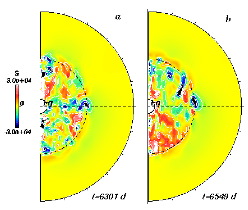
Figure 18: Variation of axisymmetric toroidal field $\left<B_{t}\right>$ with radius and latitude for case Em at two instants coinciding with Figs. 17$a$,$d$. Red and blue tones denote in turn eastward (prograde) and westward (retrograde) field.

Figure 18 shows two snapshots of the radial and latitudinal variation of the longitudinally-averaged toroidal magnetic field $\left<B_{t}\right>$ for case Em at times coincident with Figures 17a,d. We can see that $\left<B_{t}\right>$ possesses small-scale structure, with little correspondence apparent between the two time samples, indicating the complex evolution of the axisymmetric toroidal field. Mixed polarities and intricate topologies are present throughout the convective core. Varying symmetries may be evident at different instants, but do not persist over extended intervals.

Some hints regarding the interplay between the $\alpha$-effect and the $\omega$-effect in generating axisymmetric toroidal fields are afforded by comparing Figure 18 with the views of $\left<{\bf B_{p}}\right>$ in Figure 17. If the $\omega$-effect had a dominant role in the generation of $\left<B_{t}\right>$, as may be realized at the core boundary where convective motions have waned, the evolution of the axisymmetric poloidal and toroidal fields would be clearly linked. The largely retrograde differential rotation acting on a negative poloidal field structure would generate a toroidal field with two opposite polarities: negative in the lower part of the structure and positive in the upper part. That the non-axisymmetric convection also plays a role in generating $\left<B_{t}\right>$ through the $\alpha$-effect obscures the connection between structures in the two fields, yet some links are indeed revealed by Figure 18. In Figure 17$a$ the poloidal field possesses a counterclockwise (negative) polarity at mid latitudes along the convective core boundary in the northern hemisphere. The appearance in Figure 18$a$ of both senses of toroidal fields at the same location may be indicative of the $\omega$-effect at work. Similar linkages are apparent in Figure 18$b$, where the corresponding poloidal field was largely of negative polarity along the core interface but $\left<B_{t}\right>$ is largely of differing senses in the northern and southern hemispheres. Of course some time lag should exist between the establishment of toroidal mean fields from a given mean poloidal field configuration via the $\omega$-effect, further complicating the interpretation of links between the two fields. Furthermore, many departures from this idealized description of the generation of fields occur due to the major role played by the $\alpha$-effect within the core in giving rise to the magnetism.

6.3 Wandering of the Poles

Like the axisymmetric poloidal and toroidal fields, the dipole component of the magnetism attracts interest despite its relatively small amplitude. Dipole magnetic fields have figured prominently in some theoretical efforts to construct simplified models of the interiors of A-type stars (e.g., Mestel & Moss 1977). In addition, the presence at the surface of largely dipolar fields further serves to motivate the examination of such fields in our simulations, though this interior magnetism may well be screened from view by the extensive radiative envelope. We here assess the temporal variations of the dipole field, which may differ appreciably from those of the rapidly evolving and intricate small-scale fields.

In our two simulations, the maximum amplitude of the dipole magnetic field (namely the $\ell=1$ component of $B_{r}$) is generally no greater than about 5% of the maximum total radial field, with variations in strength by a factor of two occurring as the fields evolve in time. Further, the low spherical harmonic degrees $\ell=2-12$ typically possess somewhat greater amplitudes than the dipole. The evolution in case C4m of the dipole axis over a period of $\sim$1900 days (or about 270 rotations) is assessed in Figure 19, showing the position in latitude and longitude of the positive dipole axis with time. The orientation of the dipole, which is inclined with respect to the rotation axis, varies slowly: during the lengthy interval sampled, the pole completes only two full revolutions around the rotation axis, though there are brief periods during which its movement is more rapid. The wanderings from the northern hemisphere into the southern and back are similarly leisurely: only three such inversions of polarity, each separated by more than 500 days, are visible in Figure 19. The orientation of the dipole appears to correspond very well with the sign of the axisymmetric poloidal magnetic field when integrated over the northern hemisphere (Fig. 17$f$). As the dipole meanders from a northerly orientation to a southerly one, the sign of the integrated radial field at the edge of the convective core also flips from positive to negative. Similar slow wanderings are observed in case Em, though there the dipole axis lies close to the equatorial plane over the first 1500 days of the interval sampled in Figure 17$e$. Thus the slow evolution of the dipole component of the magnetism stands in contrast to the far more rapid changes seen in the high-degree components.

7 SOME ASPECTS OF FIELD GENERATION

The detailed manner in which sustained dynamo action is achieved in our models is challenging to understand, since we have relatively few theoretical tools for predicting such behavior short of carrying out nonlinear simulations. In mean-field dynamo theory (see e.g., Moffatt 1978; Brandenburg & Subramanian 2004), one commonly speaks of the $\alpha$-effect, by which helical turbulence in a resistive medium can produce mean toroidal magnetic fields from seed poloidal ones and vice versa, and of the $\omega$-effect, in which stretching of field lines by contrasts in angular velocity can generate mean toroidal fields from poloidal ones. Although the $\omega$ and $\alpha$ effects strictly refer only to the generation of mean toroidal and poloidal fields from mean and fluctuating fields, their counterparts in the equation for the evolution of the fluctuating fields may be useful in looking at the generation of the strong fluctuating fields realized in our simulations.

Among these generation terms, the G-current ${\bf G}={\bf v}^{\prime}\times{\bf B}^{\prime}-<{\bf v}^{\prime}\times{\bf B}^{\prime}>$ plays a pivotal role. In the traditional first-order smoothing approximation of mean field dynamo theory (Krause & Rädler 1980, Ossendrijver 2003), this term is neglected, providing a simple closure procedure for the mean field induction equations. We find in our simulations that the G-current is by no means small, with $<{\bf v}^{\prime}\times{\bf B}^{\prime}>$ considerably smaller (about only 5%) than ${\bf v}^{\prime}\times{\bf B}^{\prime}$. Further, the nonlinear dynamo action realized in our simulations induces preferentially strong non-axisymmetric fluctuating magnetic fields rather than axisymmetric ones, with the latter having only a very weak dynamical role. Our core convection dynamo simulations suggest that higher-order mean field dynamo theories, which do not neglect the G-current, may be required to explain the dynamo operating in a stellar convective core.

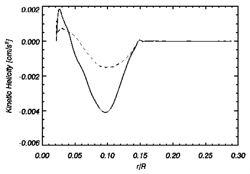
Figure 20: Kinetic helicity as a function of radius for case Em (dashed line) and its purely hydrodynamical progenitor (solid line), as averaged over the northern hemisphere and in time. The kinetic helicity is reduced in the presence of magnetism. The kinetic helicity has been averaged over 120 days in both cases given the large fluctuations that this quantity undergoes in the convective core.

A physical quantity of some interest in analyzing the properties of the magnetic field generated in our simulations is the kinetic helicity ${\bf v}\cdot(\mbox{\boldmath$\nabla$}\times{\bf v})$. In Figure 20, we display the kinetic helicity both for case Em and for its hydrodynamical progenitor as a function of radius, averaged over the northern hemisphere and in time. It is negative in most of the domain except for a positive region near the center of the core. In contrast, the current helicity ${\bf j}\cdot{\bf B}$ in our simulations shows no comparable trends or sign preference in a given hemisphere, in agreement with the results obtained in the solar dynamo simulations of Brun et al. (2004). As a consequence, we see no evident relation between the kinetic and magnetic helicities in our modeling, though some links are implicit in certain mean field theories (e.g., Ossendrijver 2003). Turning back to Figure 20, we note that the kinetic helicity in case Em possesses a smaller amplitude than in its hydrodynamic progenitor. This suggests that the magnetic field acts to reduce local shear and stretching, in particular near sites of strong vorticity, leading to a reduced helicity in the convective region. Outside the core, in the region of overshooting and beyond, the kinetic helicity is very small, since only weak fluid motions persist. Thus the generation of magnetic fields by helical convective motions must also basically vanish outside the core.

Conversely, angular velocity contrasts that are weak within the convective core grow stronger in the region of overshooting, particularly in case Em with its interface of strong shear. Thus the balance of toroidal and poloidal field should vary with radius, as the relative importance of the helical motions grows smaller and the contribution of the large-scale shear becomes larger. The radial variation of the energy in the fluctuating and axisymmetric magnetic fields (§5.1) therefore provides clues about the mechanisms responsible for building the magnetism. Although the total ME declines sharply outside the convective core, the axisymmetric toroidal field $\hat{B}_{\phi}$ within the region of overshooting is still considerable. This, together with the longitudinally elongated topology of $\hat{B}_{\phi}$ (Fig. 3$c$), indicates that the large-scale shear helps generate the magnetism. That TME exceeds PME by a factor of two within the convective core suggests that the equivalent of an $\omega$-effect plays a role there as well. These core convection dynamos thus generate magnetic fields through the joint effects of large-scale shear and helical motions acting on the axisymmetric and the non-axisymetric fields. The large-scale shear appears to dominate the generation of field near the convective core boundary, while the helical motions generate fields in a more distributed manner within the core.

8 CONCLUSIONS AND PERSPECTIVES

The simulations here reveal that vigorous convection within the cores of rotating A-type stars can serve to build strong magnetic fields through dynamo action. Small initial seed magnetic fields are amplified in strength by many orders of magnitude and sustained against ohmic decay, ultimately yielding fields that are nearly in equipartition with the flows. The resulting highly time-dependent magnetism possesses structure on many scales, with $B_{r}$ mainly fibril and $B_{\phi}$ stretched by the zonal flows (differential rotation) into large-scale bands that extend around the core. Within the core, the magnetism is predominantly fluctuating, with such non-axisymmetric fields accounting for about 90% of the total magnetic energy. The accompanying weak mean (axisymmetric) fields evolve comparatively slowly, undergoing flips in average polarity on time scales of hundreds of days. In the farther region of overshooting and beyond, where the magnetic energy plummets from its interior value, the mean toroidal field becomes the dominant component of the surviving magnetism.

The differential rotation established in the hydrodynamic progenitors is lessened in latitude by the presence of magnetism, as the strong Maxwell stresses associated with the fluctuating fields transport angular momentum poleward, with the large-scale magnetic torques playing only a small role in the overall latitudinal balance. Conversely, the radial transport of angular momentum by the Maxwell stresses does not oppose that of the Reynolds stresses throughout much of the convective core. Thus the Maxwell stresses are found to play a significant role in the angular momentum transport. In case Em, with ME about 40% of KE, central columns of slow rotation are still realized, with considerable variations in strength as the simulations evolve. Oscillations seen in the energy densities DRKE and ME (Fig. 10) hint at the intimate connection between magnetic fields and flows, with intervals of high ME apparently acting to quench the differential rotation; the resulting weak angular velocity contrasts eventually lead to decreases in ME. In case C4m rotating at four times the solar rate, in which ME at times exceeds KE (Fig. 2), angular velocity contrasts are always weaker than in case Em that rotates at the solar rate (Fig. 9). Similar damping of the differential rotation by the Lorentz forces is also realized to a lesser extent in 3-D MHD simulations of the solar convection zone (Brun et al. 2004; Brun 2004).

How the magnetism is built and sustained by the flows is an intricate matter. Both the helical convection and the differential rotation have significant roles, with axisymmetric fields generated in the core through processes somewhat akin to the $\alpha$- and $\omega$-effects of mean-field dynamo theory. It would appear that the two effects contribute in roughly equal measure to building axisymmetric toroidal fields within the core, as indicated by MTE sampled at mid-core exceeding MPE by a factor of about two in case Em (Table 3). The role of helical convection here in generating field is unlike that prescribed in the simpler variants of mean-field theory (i.e., the first-order smoothing approximation). In particular, the fluctuating field $B^{\prime}$ in our simulations is not proportional to the longitudinally-averaged field $<B>$, possibly because the G-current is not small. This may explain the absence of a linear relationship between the fluctuating and axisymmetric fields in our modeling. In the radiative envelope, convective motions do not persist and so cannot serve to build magnetism, but weak angular velocity contrasts continue to generate axisymmetric toroidal magnetic fields through stretching via the $\omega$-effect. Thus MTE with increasing radius comes to dominate over both FME and MPE, as seen in Figure 14.

We also find that the magnetic energy peaks slightly at the bottom of the convective domains due to the downward transport of magnetic fields by the convection. This is in sharp contrast with the much more peaked profile found in our simulation of the solar dynamo (Brun et al. 2004), where the asymmetry between weak upflows and strong downflows is more pronounced due to a stronger density contrast there.

The intense and rapidly evolving magnetism realized within the core is screened by the extensive radiative envelope, so assessing its possible impact at the stellar surface is difficult. The complex morphologies of the magnetic fields, their periodic reversals in mean polarity, and their intimate feedback upon the turbulent convection may all be hidden from view. If diffusion alone served to bring the magnetic fields outward from the core, the rapid temporal variations (and so too the intricate spatial structure) of the core fields would be obliterated by the characteristic diffusive time scales of order millions of years.

Whether the fields could migrate to the surface by means other than diffusion, and thus perhaps contribute to the observed magnetism of Ap stars, has been the subject of some debate. Magnetic buoyancy instabilities at the edge of the core could conceivably bring the fields to the surface much more rapidly than diffusion. We cannot address the rise of such buoyant flux tubes directly in our simulations, since we model only the interior portions of these stars at resolutions insufficient to capture the highly concentrated structures needed for these instabilities to act. However, MacGregor & Cassinelli (2003) have used simple models to consider how buoyant magnetic structures may traverse the radiative exterior. They deduce that magnetism from the core could arrive at the stellar surface in less than the main-sequence lifetime of an A-type stars if the interior fields were both very strong and highly fibril. Further modeling by MacDonald & Mullan (2004) suggests that the presence of compositional gradients would slow this process considerably. Furthermore, the field strengths likely to be realized at the surface from such buoyant flux tubes are only modest (MacGregor & Cassinelli 2003), in contrast with the kG fields that are observed in some Ap stars. The implications of these recent studies remain somewhat unclear, for several effects that might modify the rise of buoyant core magnetic fields have yet to be included, among them global-scale circulations within the radiative envelope and the twist and writhe of the flux tubes that could modify their stability. The strong surface fields also appear to occupy large sectors, which might be very difficult to populate through the rise of individual elements. Invoking fossil origins for the observed surface magnetism, with predominate dipole structure surviving, is a favored explanation (e.g., Moss 2001) since strong fields could more easily be obtained. The interaction of the interior magnetism with such possible large-scale fossil fields has also not yet been seriously studied. However, the alternative possibility that the radiative envelope could induce a magnetic field via dynamo action (Spruit 2002; MacDonald & Mullan 2004) may encourage reconsideration of that scenario. Also, the generation by the overshooting convection of internal waves could potentially play a role in the radiative zone, creating shear layers that could subsequently amplify a magnetic field (Kumar, Talon & Zahn 1999).

Future work will thus be required to explore in detail the possible role of the core convection dynamo in giving rise to the surface magnetism. Likewise we have only briefly touched the possible variations with rotation of the dynamo action and differential rotation. Our limited sampling of two rotation rates provides some hints at that variation (i.e., the faster case C4m possesses a stronger magnetic field than case Em), but does not elucidate it, for we have explored only one avenue in the vast parameter space that could be relevant to real stars. Indeed, the detailed nature of the flows and magnetism in our simulations is surely affected by the many approximations we have made in considering these stars. How the far more turbulent flows attained in actual stars impact the generation of magnetic fields and differential rotation is quite uncertain. Yet some of the dominant features found here may well turn out to be robust. The conclusion that core convection drives some form of sustained dynamo action, producing very strong fields that feed back on the flows, appears to us to be inescapable.

This work was partly supported by NASA through SEC Theory Program grant NAG5-11879, and through the Graduate Student Researchers Program (NGT5-50416). The simulations were carried out with NSF PACI support of the San Diego Supercomputing Center (SDSC), the National Center for Supercomputing Applications (NCSA), and the Pittsburgh Supercomputing Center (PSC) as well as with the Centre de Calcul pour la Recherche et la Technologie (CCRT) of CEA at Bruyère-le-Chatel and within the CNRS supercomputers center IDRIS. Much of the analyses were conducted in the Laboratory for Computational Dynamics (LCD) within JILA. One of us (ASB) is grateful to R. Grappin and J.-P. Zahn for interesting discussions and insights on turbulent MHD.

Table 1: Parameters for Magnetic Simulations

Case	Em	C4m
	Input parameters
$N_{r},N_{\theta},N_{\phi}$	82, 256, 512	82, 256, 512
$\Omega_{0}$ (s-1)	$2.6\times 10^{-6}$	$1.04\times 10^{-5}$
$R_{a}$	3.1 $\times 10^{5}$	1.3 $\times 10^{7}$
$P_{m}$	5	5
$R_{c}$	0.33	0.12
$\nu$ (cm2 s-1)	$4.4\times 10^{11}$	$2.5\times 10^{11}$
$\kappa$ (cm2 s-1)	$1.7\times 10^{12}$	$9.9\times 10^{11}$
$\eta$ (cm2 s-1)	$8.7\times 10^{10}$	$5.0\times 10^{10}$
$\tau_{\eta}$ (days)	3900	6800
	Measured at mid-depth of convective core
$R_{e}$	160	210
$R_{m}$	800	1050
$\Lambda$	23.2	17.8
$P_{e}$	40	52
$R_{o}$	$3.5\times 10^{-2}$	$6.2\times 10^{-3}$

Note. — The number of radial, latitudinal and longitudinal mesh points are $N_{r},N_{\theta},N_{\phi}$. All simulations have an inner radius $r_{bot}=3.0\times 10^{9}$ cm and an outer radius $r_{top}=4.0\times 10^{10}$ cm, with $L=1.7\times 10^{10}$ cm the approximate radial extent of the convective core. The overall radius $R$ of the A-type star is $1.4\times 10^{11}$ cm. The effective viscosity $\nu$, thermal diffusivity $\kappa$, and magnetic diffusivity $\eta$ are quoted at the middle of the convective core ($r=0.10R$), and likewise we evaluate there the Rayleigh number $R_{a}=(-\partial\bar{\rho}/\partial S)\Delta SgL^{3}/\rho\nu\kappa$ (with $\Delta S$ the entropy contrast across the core), the magnetic Prandtl number $P_{m}=\nu/\eta$, the convective Rossby number $R_{c}=\sqrt{R_{a}/T_{a}P_{r}}$, the Reynolds number $R_{e}=\tilde{v}^{\prime}L/\nu$, the magnetic Reynolds number $R_{m}=\tilde{v}^{\prime}L/\eta$, the Elsasser number $\Lambda=\tilde{B}^{2}/4\pi\rho\eta\Omega_{0}$, the Péclet number $P_{e}=R_{e}P_{r}=\tilde{v}^{\prime}L/\kappa$, the Rossby number $R_{o}=\tilde{v}^{\prime}/2\Omega_{0}L$, and the ohmic diffusion time $\tau_{\eta}=L^{2}/(\pi^{2}\eta)$, where $\tilde{v}^{\prime}$ is the rms fluctuating convective velocity and $\tilde{B}$ is the rms magnetic field (see Table 2 and §2.3). An $R_{e}$ based on the peak velocity at mid-depth would be about a factor of 5 larger. The Prandtl number $P_{r}=\nu/\kappa$ = 0.25 over the full depth range.

Table 2: Velocity and Magnetic Field Amplitudes

Case	Em	C4m	E	C4
$\tilde{v}_{r}$	20	15	26	19
$\tilde{v}_{\theta}$	22	16	23	16
$\tilde{v}_{\phi}$	22	21	43	72
$\tilde{v}_{\phi}^{\prime}$	20	15	21	21
$\tilde{v}$	37	30	55	76
$\tilde{v}^{\prime}$	36	26	38	32
$\tilde{B}_{r}$	28	33	-	-
$\tilde{B}_{\theta}$	30	36	-	-
$\tilde{B}_{\phi}$	28	45	-	-
$\tilde{B}_{\phi}^{\prime}$	27	44	-	-
$\tilde{B}$	50	67	-	-
$\tilde{B}^{\prime}$	49	65	-	-

Note. — Listed for both MHD simulations (cases Em, C4m) and their hydrodynamic progenitors (cases E, C4) are the rms amplitude of the velocity $\tilde{v}$ and each of its components, $\tilde{v}_{r}$, $\tilde{v}_{\theta}$, and $\tilde{v}_{\phi}$, averaged over time and over a spherical surface at mid-depth in the convective core (at $r=0.10R$). Also listed are the rms amplitudes of the fluctuating velocity $\tilde{v}^{\prime}$ and its zonal component $\tilde{v}_{\phi}^{\prime}$, averaged in time and obtained after subtracting the longitudinal average. We also indicate (where appropriate) the corresponding rms amplitudes of the magnetic field and its components, $\tilde{B}$, $\tilde{B}_{r}$, $\tilde{B}_{\theta}$, $\tilde{B}_{\phi}$, $\tilde{B}^{\prime}$, and $\tilde{B}_{\phi}^{\prime}$. Velocities are expressed in m s^-1 and magnetic fields in $kG$.

Table 3: Energy densities

Case	Em	C4m	E	C4
KE	4.54$\times 10^{7}$	1.76$\times 10^{7}$	7.58$\times 10^{7}$	1.67$\times 10^{8}$
DRKE/KE	18.2%	28.3%	56.1%	88.3%
MCKE/KE	1.9%	0.2%	1.8%	0.2%
CKE/KE	79.9%	71.5%	42.2%	11.5%
ME/KE	28.3%	88.2%	-	-
MTE/MEc	3.4%	2.7%	-	-
MPE/MEc	1.4%	2.5%	-	-
FME/MEc	94.4%	94.7%	-	-
MEc	1.27$\times 10^{8}$	2.20$\times 10^{8}$
MTE/MEr	91.3%	98.1%	-	-
MPE/MEr	0.2%	0.1%	-	-
FME/MEr	9.6%	1.8%	-	-
MEr	6.85$\times 10^{3}$	4.93$\times 10^{3}$	-	-

Note. — The kinetic energy density KE ($1/2~{}\bar{\rho}v^{2}$), averaged over volume and time, is listed along with the relative contributions from the convection (CKE), the differential rotation (DRKE), and the meridional circulation (MCKE), together with the average magnetic energy density ME ($B^{2}/8\pi$) (where appropriate). The relative contributions from each of the components of ME, including the fluctuating field FME and the axisymmetric $m=0$ toroidal and poloidal fields (MTE and MPE), are evaluated both within the radiative zone (at $r=0.24R$, denoted by $r$) and the convective core (at $r=0.10R$, denoted $c$), along with the values of ME at those two depths.

Figure 12: Temporal average in case Em of (a) the integrated vertical angular momentum flux $I_{r}$ and (b) the integrated latitudinal angular momentum flux $I_{\theta}$. These have been decomposed into components due to viscous transport (labeled VT), Reynolds stress (RS), meridional circulation (MC), Maxwell stress (MS), and large-scale magnetic torque (MT), and the solid curves represent the total fluxes. Positive quantities represent fluxes radially outward, or latitudinally from north to south. The interval chosen for the time averages spans 300 days late in the simulation.

Figure 13: Variation with radius of the radial transport of energy in case C4m, as averaged over an interval of about 60 days. Shown are the enthalpy flux $F_{e}$, the radiative flux $F_{r}$, and the Poynting flux $F_{m}$, together with the total flux $F_{t}$; all quantities have been expressed as luminosities. The convective core extends here to about $r=0.14R$, with the positive $F_{e}$ there serving to carry as much as 80% of the total flux. The further region of overshooting involves a small negative (inward directed) enthalpy flux. Here $F_{m}$ is small throughout the domain.

Figure 14: Radial variation of magnetic energy components in case C4m. Shown are the energy in the mean (axisymmetric) toroidal field (TME), the mean poloidal field (PME), and the fluctuating (non-axisymmetric) fields (FME), together with their sum (ME), all averaged over radial surfaces and in time. In the convective core, FME accounts for most of ME. Outside the core, TME becomes the dominant component in the plummeting ME.

Figure 17: ($a$)–($d$) Temporal evolution of the axisymmetric (mean) poloidal field $\left<{\bf B_{p}}\right>$ for case Em, shown as meridional cross section at four selected times indicated. Solid contours denote positive polarity (field lines directed from north to south) and dotted contours denote negative polarity. ($e$) The accompanying radial field for case Em at the convective core boundary (solid line) and at the top of the domain (dashed) as averaged over the northern hemisphere, shown over 2400 days late in the simulation with timings of upper snapshots denoted. ($f$) Temporal evolution of average polarity of $B_{r}$, as in ($e$), for case C4m.

Figure 19: Wandering of the magnetic dipole axis in case C4m with time. ($a$) Its position with latitude as the field swings between the northern and southern hemispheres. ($b$) The gradual drift in longitude of the positive pole.

References

- (1) Bagnulo, S., Landstreet, J.D., LoCurto, G., Szeifert, T. & Wade, G.A. 2003, A&A, 403, 645
- (2) Biskamp, D. 1993, Nonlinear Magnetohydrodynamics (Cambridge: Cambridge Univ. Press)
- (3) Borra, E.F. 1980, ApJ, 235, 915
- (4) Borra, E.F. & Landstreet, J.D. 1980, ApJS, 42, 421
- (5) Brandenburg, A., Jennings, R. L., Nordlund, Å., Rieutord, M., Stein, R. F., Tuominen, I. 1996, JFM, 306, 325
- (6) Brandenburg, A., & Subramanian, K. 2004, astro-ph/0405052
- (7) Browning, M., Brun, A.S., & Toomre, J. 2005, in Stellar Rotation, Proc. IAU Symp. 215, ed: A. Maeder & P. Eenens (San Francisco: ASP), in press
- (8) Browning, M. K., Brun, A. S., & Toomre, J. 2004, ApJ, 601, 512
- (9) Brun, A. S. 2004, Solar Phys., 220, 333
- (10) Brun, A.S., & Toomre, J. 2002, ApJ, 570, 865
- (11) Brun, A.S., Browning, M. K., & Toomre, J. 2005, in Stellar Rotation, Proc. IAU Symp. 215, ed: A. Maeder & P. Eenens (San Francisco: ASP), in press
- (12) Brun, A.S., Miesch, M.S., & Toomre, J. 2004, ApJ, 614, in press
- (13) Castaing, B., Gagne, Y., & Hopfinger, E. J. 1990, Physica D, 46, 177
- (14) Chandrasekhar, S. 1961, Hydrodynamic and Hydromagnetic Stability (Oxford:Clarendon)
- (15) Charbonneau, P., & MacGregor, K.B. 1997, ApJ, 486, 502
- (16) Clune, T.L., Elliott, J.R., Glatzmaier, G.A., Miesch, M.S., & Toomre, J. 1999, Parallel Computing, 25, 361
- (17) Elliott, J.R., Miesch, M.S., & Toomre, J. 2000, ApJ, 533, 546
- (18) Frisch, U. 1995, Turbulence: The legacy of A.N. Kolmogorov (Cambridge: Cambridge University Press)
- (19) Gilman, P.A. 1983, ApJS, 53, 243
- (20) Grappin, R., Léorat, J. & Pouquet, A. 1983, A&A, 126, 51
- (21) Hubrig, S., North, P., & Mathys, G. 2000, ApJ, 539, 352
- (22) Jackson, J. D. 1999, Classical Electrodynamics 3rd ed, ed Wiley
- (23) Kochukhov, O., Bagnulo, S., Wade, G., Sangalli, L., Piskunov, N., Landstreet, J.D., Petit, P. & Sigut, T.A.A. 2004, A&A, 414, 613
- (24) Krause, F. & Rädler, K.-H. 1980, Mean-Field Magnetohydrodynamics and Dynamo Theory, (1st ed; Oxford: Pergamon Press)
- (25) Krause, F. & Oetken, L. 1976, in Physics of Ap Star, ed.: W.W. Weiss, H. Jenkner, & H.J. Wood (Vienna: Universitatssternwarte Wien), 29
- (26) Kumar, P., Talon, S., & Zahn, J.-P. 1999, ApJ, 520, 859
- (27) Lamballais, E., Lesieur, M., & Métais, O. 1997, Phys. Rev. E, 56, 6761
- (28) MacDonald, J., & Mullan, D.J. 2004, MNRAS, 348, 702
- (29) MacGregor, K.B., & Cassinelli, J.P. 2003, ApJ, 586, 480
- (30) Maury, A.C. 1897, Harvard Ann., 28, 96
- (31) Mestel, L. 1999, Stellar Magnetism, (Oxford: Clarendon)
- (32) Mestel, L., & Moss, D.L. 1977, MNRAS, 178, 27
- (33) Miesch, M.S., Elliott, J.R., Toomre, J., Clune, T.L., Glatzmaier, G.A., & Gilman, P.A. 2000, ApJ, 532, 593
- (34) Moffatt, H.K. 1978, Magnetic Field Generation in Electrically Conducting Fluids, ed. Cambridge University Press
- (35) Moss, D.L. 1989, MNRAS, 236, 629
- (36) Moss, D.L. 1992, MNRAS, 257, 593
- (37) Moss, D.L. 2001, in Magnetic Fields Across the Hertzsprung-Russell Diagram, ed: G. Mathys, S.K. Solanki, & D.T. Wickramasinghe (San Francisco:ASP), 305
- (38) Moss, D.L., Mestel, L., & Tayler, R.J. 1990, MNRAS, 245, 550
- (39) Ossendrijver, M. 2003, Astron. Astrophys. Rev., 11, 287
- (40) Pedlosky, J. 1987, Geophysical Fluid Dynamics (New York: Springer-Verlag)
- (41) Spruit, H.C. 2002, A&A, 381, 923
- (42) Stibbs, D.W.N. 1950, MNRAS, 110, 395
- (43) Vincent, A., & Meneguzzi, M. 1991, J. Fluid Mech., 225, 1
- (44) Wolff, S.C. 1983, The A-stars: Problems and perspectives, (Washington, D.C.: NASA)