Empirical strong-line oxygen abundance calibrations from galaxies with electron temperature measurements

Abstract

Context.

Aims. We determine the gas-phase oxygen abundance for a sample of 695 galaxies and H ii regions with reliable detections of [O iii]4363, using the temperature-sensitive ($T_{e}$) method, which is the most reliable and direct way of measuring metallicity. Our aims are to estimate the validity of empirical methods such as $R_{23}$, $R_{23}-P$, log([N ii]/H$\alpha$) (N2), log[([O iii]/H$\beta$)/([N ii]/H$\alpha$)] (O3N2), and log([S ii]/H$\alpha$) (S2), and re-derive (or add) the calibrations of $R_{23}$, N2, O3N2 and S2 indices for oxygen abundances on the basis of this large sample of galaxies with $T_{e}$-based abundances.

Methods. We select 531 star-forming galaxies from the Fourth Data Release of the Sloan Digital Sky Survey database (SDSS-DR4) with strong emission lines, including [O iii]4363 detected at a signal-to-noise larger than 5$\sigma$, as well as 164 galaxies and H ii regions from literature with $T_{e}$ measurements. O/H abundances have been derived from a two-zone model for the temperature structure, assuming a relationship between high ionization and low ionization species.

Results. We compare our (O/H)${}_{T_{e}}$ measurements of the SDSS sample with the abundances obtained by the MPA/JHU group using multiple strong emission lines and Bayesian techniques (Tremonti et al. 2004). For roughly half of the sample the Bayesian abundances are overestimated $\sim$0.34 dex, possibly due to the treatment of nitrogen enrichment in the models they used. $R_{23}$ and $R_{23}-P$ methods systematically overestimate the O/H abundance by a factor of $\sim$0.20 dex and $\sim$0.06 dex, respectively. The N2 index, rather than the O3N2 index, provides more consistent O/H abundances with the $T_{e}$-method, but with some scatter. The relations of N2, O3N2, S2 with log(O/H) are consistent with the photoionization model calculations of Kewley & Doptita (2002), but $R_{23}$ does not match well. We derive analytical calibrations for O/H from $R_{23}$, N2, O3N2 and S2 indices on the basis of this large sample, as well including the excitation parameter $P$ as an additional parameter in the N2 calibration. These empirical calibrations are free from the systematic problems inherent in abundance calibrations based on photoionizatoin models.

Conclusions. We conclude that, the N2, O3N2 and S2 indices are useful indicators to calibrate metallicities of galaxies with 12 + log(O/H) $<$ 8.5, and the $R_{23}$ index works well for the metal-poor galaxies with 12+log(O/H)$<$7.9. For the intermediate metallicity range (7.9 $<$ 12 + log(O/H) $<$ 8.4), the $R_{23}$ and $R_{23}-P$ methods are unreliable to characterize the O/H abundances.

1 Introduction

The chemical properties of stars and gas within a galaxy provides both a fossil record of its star formation history and information on its present evolutionary status. It is therefore desirable to extract as much, and as accurate, information as possible from observations of galaxies. In particular it is important that different methods for extracting information provides this without systematic offsets, or at the very least that these systematic offsets are well understood. Accurate abundance measurements for the ionized gas in galaxies require the determination of the electron temperature ($T_{e}$) in this gas which is usually obtained from the ratio of auroral to nebular line intensities, such as [O iii]$\lambda\lambda 4959,5007$/[O iii]$\lambda$4363. This is generally known as the “direct $T_{e}$-method” because the electron temperature is directly inferred from observed line ratios. It is well known that this procedure is difficult to carry out for metal-rich galaxies since, as the metallicity increases, the electron temperature decreases (as the cooling is via metal lines) and the auroral lines eventually become too faint to measure. Instead, the most common method used for estimating oxygen abundance of metal-rich galaxies (12+log(O/H)$\geq$8.5) uses the $R_{23}$ (=([O ii]$\lambda$3727+[O iii]$\lambda\lambda$4959,5007)/H$\beta$) parameter, which is the ratio of the flux in the strong optical oxygen lines to that of H$\beta$ (Pagel et al. 1979; Tremonti et al. 2004 and the references therein). The $R_{23}$ indicator can also be used for metal-poor galaxies (12+log(O/H)$<$8.5) (Skillman et al. 1989; Kobulnicky et al. 1999; McGaugh 1991; Pilyugin 2000; Edmunds & Pagel 1984).

Several researchers have however found that $R_{23}$-derived abundances are inconsistent with the $T_{e}$-derived ones, showing a systematic offset. For example, Kennicutt et al. (2003) found that $R_{23}$ will overestimate the actual log(O/H) abundance by a factor of 0.2-0.5 dex using a sample of 20 H ii regions in M101 with high-S/N spectra. Some other researches found the similar results, for example, Bresolin et al. (2004, 2005), Garnett et al. (2004a,b), Pilyugin (2006), Shi et al. (2005, 2006). A much larger dataset can help to understand better this effect and extending it to galaxies will also be of considerable interest.

To estimate abundances of galaxies, when $T_{e}$ and $R_{23}$ cannot be used, some other metallicity-sensitive “strong-line” ratios are very useful, for example, [N ii]$\lambda$6583/H$\alpha$, [O iii]$\lambda$5007/[N ii]$\lambda$6583, [N ii]$\lambda$6583/[O ii]$\lambda$3727, [N ii]$\lambda$6583/[S ii]$\lambda\lambda$6717,6731, [S ii]$\lambda\lambda$6717,6731/H$\alpha$, and [O iii]$\lambda\lambda$4959,5007/H$\beta$ (Liang et al. 2006; Nagao et al. 2006; Pérez-Montero & Díaz 2005; Pettini & Pagel 2004, hereafter PP04; Denicol$\acute{o}$ et al. 2002, hereafter D02; Kewley & Dopita 2002, hereafter KD02). Even when $R_{23}$ is available, some of these line-ratios are useful to overcome the well-known problem that the $R_{23}$ vs. 12 + $\log$O/H relation is double-valued and further information is required to break this degeneracy. Alternative methods for breaking the degeneracy when a well established luminosity-metallicity relation exists, or when the likelihood of each branch can be calculated, which has been discussed by Lamareille et al. (2006).

Strong-line abundance indicators are typically calibrated in one of two ways: (1) using the samples of galaxies with direct ($T_{e}$-based) abundances (e.g. PP04; Pagel et al. 1979 etc.); (2) using photoionization models (e.g. McGaugh 1991; Tremonti et al. 2004 etc.). Since the $T_{e}$-method is generally thought to be the most accurate method for metallicity estimation, we will take oxygen abundances derived using this method as our baseline. We select a large sample of 531 galaxies from the SDSS-DR4 with their [O iii]$\lambda$4363 emission line detected at a S/N ratio greater than 5$\sigma$, and 164 associated galaxies and H ii regions from literature. We compare their $T_{e}$-based O/H abundances with the Bayesian estimates provided by the MPA/JHU group (shown as log(O/H)_Bay), which were obtained by fitting multi-emission lines using the photoionization models of Charlot et al. (2006), and with those derived from some strong-line ratios given in previous studies, including $R_{23}$, $P$, N2 and O3N2 methods etc. (Kobulnicky et al. 1999; Pilyugin 2001; PP04). We also compare the observational results with the photoionization model results of KD02 for the relations of O/H vs. $R_{23}$, N2, O3N2 and S2 indices.

Specially, we study the abundance calibrations of strong-line ratios on the basis of their $T_{e}$-based metallicities. When we compare the observational relations of O/H vs. strong-line ratios with the photoionization model results of KD02, we find that only the N2, O3N2, S2 indices are useful to estimate abundances for galaxies with low metallicity, 12+log(O/H)${}_{T_{e}}$$<$8.5, while other line ratios, such as [N ii]/[O ii], [N ii]/[S ii] are [O iii]/H$\beta$ are not good indicators for this metallicity range due to their insensitivity to metallicities there, except in the extremely metal-poor environments (e.g. 12+log(O/H)$<$7.5 or 7.0) (Stasińska 2002; KD02). $R_{23}$ is a useful indicator of metallicity for the low metallicity region with 12+log(O/H)$<$7.9. Thus, we will only calibrate the relationships of the $R_{23}$, N2, O3N2 and S2 indices to O/H abundances from the observational data in this study. Moreover, for the N2 index, we follow Pilyugin (2000;2001a,b) to add the excitation parameter $P$ (=[O iii]/([O ii]+[O iii])) to separate the sample galaxies into three sub-samples in the calibrations. These calibrations can be the extension of the metal-rich region studied by Liang et al. (2006) to the low metallicity region.

This paper is organized as follows. The sample selection criteria are described in Sect. 2. The determinations of the oxygen abundances from $T_{e}$ are presented in Sect. 3. In Sect. 4, we present the comparisons between the (O/H)${}_{T_{e}}$ and the (O/H)_Bay, as well as those abundances derived from other strong-line relations. Sect. 5 shows the comparison of the observational data with the photoionization models of KD02. In Sect.6, we re-derive analytical calibrations between O/H and $R_{23}$, N2, O3N2, S2 indices, as well the two-parameter calibrations for the N2 index with $P$-parameter included. The conclusions are given in Sect. 7.

2 Observational data

2.1 The SDSS-DR4 data

The SDSS-DR4 (Adelman-McCarthy et al 2006) provides spectra in the wavelength range $\sim$ 3800–9200Å for $>$ 500,000 galaxies over 4783 square degrees. The MPA-JHU collaboration has in addition made measurements of emission-line fluxes and some derived physical parameters for a sample of 520,082 unique galaxies at the MPA SDSS website. Therefore, we will call the working sample selected in this study as the “MPA/JHU sample” hereafter. We select the “star-forming galaxies” with metallicity measurements, which have been identified following the selection criteria of the traditional line diagnostic diagram [N ii]/H$\alpha$ vs. [O iii]/H$\beta$ (Baldwin et al. 1981; Veilleux & Osterbrock 1987; Kewley et al. 2001; Kauffmann et al. 2003). The fluxes of emission-lines have been measured from the stellar-feature subtracted spectra with the spectral population synthesis code of Bruzual & Charlot (2003) (Brinchmann et al. 2004; Tremonti et al. 2004).

We select the galaxies with redshifts 0.03$<z<$0.25 to ensure to cover from [O ii] to H$\alpha$ and [S ii] emission lines. Tremonti et al. (2004) also discussed the weak effect of aperture on estimated metallicities of the sample galaxies with $0.03<z<0.25$ and this was further discussed by Kewley et al. (2005), but for the present study the aperture effects are unimportant.

In this study, we use the $T_{e}$-method to derive O/H abundances of the sample galaxies (see Sect. 3 for details), therefore, we select the samples with [O iii]$\lambda$4363 emission-line detected at a S/N ratio greater than 5$\sigma$. To be consistent with Liang et al. (2006) and Tremonti et al. (2004), we also consider the objects having been measured fluxes of [O ii]$\lambda\lambda$3726,3729, [O iii]$\lambda$5007, H$\beta$, H$\alpha$, [N ii]$\lambda 6583$, [S ii]$\lambda\lambda 6717,6731$ emission lines, and the S/N ratio of H$\beta$, H$\alpha$, [N ii], [S ii] are larger than 5$\sigma$. The final sample consists of 531 galaxies. These have fluxes in [O iii]$\lambda$4363 greater than 5.3$\times$10^-17 ergs s^-1 cm^-2, with a mean value of 21.27 $\times$10^-17 ergs s^-1 cm^-2.

The fluxes of the emission lines are corrected for dust extinction, which are estimated using the Balmer line ratio H$\alpha$/H$\beta$: assuming case B recombination, with a density of 100 cm^-3 and a temperature of $10^{4}$ K, and the intrinsic ratio of H$\alpha$/H$\beta$ is 2.86 (Osterbrock 1989), with the relation of $(\frac{I_{H\alpha}}{I_{H\beta}})_{obs}$= $(\frac{I_{H\alpha 0}}{I_{H\beta 0}})_{intr}$10^{-c(f(Hα)-f(Hβ))}. Using the average interstellar extinction law given by Osterbrock(1989), we have $f$(H$\alpha$)- $f$(H$\beta$) = -0.37. For the 56 data points with $c<0$, we assume they have $c$ = 0 since their intrinsic H$\alpha$/H$\beta$ may be lower than 2.86 if their electron temperature is high (Osterbrock 1989, p.80).

Nearly all previous empirical oxygen abundance calibrations have been derived from individual H ii regions since it is much easier to detect [O iii]4363 that way. In contrast the SDSS data samples the inner few kpc of most galaxies. One question is whether the global spectrum from a mixture of different H ii regions will yield meaningful average abundances of the galaxies or not. Kobulnicky et al. (1999), Moustakas & Kennicutt (2006) and Pilyugin et al. (2004) concluded that the spatially unresolved emission-line spectra can reliably indicate the chemical properties of distant star-forming galaxies. However, as Kobulnicky et al. (1999) mentioned, the standard nebular chemical abundance measurement methods may be subject to small systematic errors when the observed volume includes a mixture of gas with diverse temperatures, ionization parameters, and metallicities. For the low-mass, metal-poor galaxies, as those we are studying in this work, standard chemical analyses using global spectra will overestimate the electron temperatures $T_{e}$ due to the non-uniform $T_{e}$ and large variations in the ionization parameter since the global spectra are biased to the objects with stronger emission lines. As a result, the oxygen abundances derived from $T_{e}$ will be underestimated, i.e. about $<$0.1 dex in log(O/H) (for more massive metal-rich galaxies like local spiral galaxies, it is about $\pm$0.2 dex discrepancy). However, since this bias is small, and not well constrained for our dataset, we do not attempt to correct for it.

2.2 The metal-poor galaxies from literature

In addition to the MPA/JHU samples, we also collect 164 low-metallicity samples including some blue compact galaxies (BCDs) and H ii regions from literature, which are taken from Izotov et al. (1994, 1996, 1997a, 1997b, 1998a, 1998b, 1999a, 2001a, 2001b, 2004a, 2004b), van Zee (2000), Kniazev et al. (2000), Vilchez et al. (2003), Guseva et al. (2003a,b,c), Melbourne et al. (2004), and Lee et al. (2004). There are 110 H ii regions and 54 galaxies in this sample.

We re-estimate their O/H abundances by using the electronic temperatures method given in Sect. 3. Their metallicities are 7.1$<$12+log(O/H)$<$8.4, more metal-poor than the SDSS galaxies generally.

To check if there is systematic difference between our estimates and the values given in the previous studies, we compare their $T_{e}$-based oxygen abundances obtained by us with those $T_{e}$-based given in the original reference in Fig. 1, which shows that they are very consistent, and the very slight difference may come from different atomic data.

Figure 1: Comparison between the $T_{e}$-based oxygen abundances (this work) and those from literature.

3 Abundance determination from $T_{e}$

A two-zone model for the temperature structure within the H ii region was adopted. In this model, $T_{e}$([O iii]) is taken to represent the temperature for high-ionization species such as $O^{++}$, while $T_{e}$([O ii]) is used for low-ionization species such as $O^{+}$. The general method is firstly to derive $t_{3}$ (=10${}^{-4}T_{e}$([O iii])) from the emission-line ratio of [O iii]4959,5007/[O iii]4363, and then to estimate $t_{2}$ (=10${}^{-4}T_{e}$([O ii])) from an analytical relation between $t_{2}$ and $t_{3}$ inferred from photoionization calculations.

Izotov et al. (2005) have recently published a set of equations for the determination of the oxygen abundances in H ii regions for a five-level atom. They used the atomic data from the references listed in Stasińska (2005). According to those authors, the electron temperature $t_{3}$ (in units of $10^{4}$ K), and the ionic abundances $O^{++}/H^{+}$ and $O^{+}/H^{+}$ are estimated as follows:

$$t_{3}=\frac{1.432}{{\rm log}((\lambda 4959+\lambda 5007)/\lambda 4363)-{\rm log}C_{T}},$$ (1)

where

$$C_{T}=(8.44-1.09t_{3}+0.5t_{3}^{2}-0.08t_{3}^{3})\frac{1+0.0004x_{3}}{1+0.044x_{3}},$$ (2)

with $x_{3}=10^{-4}n_{e}t_{3}^{-1/2}$, and $n_{e}$ is the electron density in cm^-3. And

$$12+{\rm log}(O^{++}/H^{+})={\rm log}(I_{{[O}{III]\lambda 4959+\lambda 5007}}/I_{H\beta})+$$

$$6.200+\frac{1.251}{t_{3}}-0.55{\rm log}t_{3}-0.014t_{3},$$ (3)

$$12+{\rm log}(O^{+}/H^{+})={\rm log}(I_{{[O}{III]\lambda 3726+\lambda 3729}}/I_{H\beta})+$$

$$5.961+\frac{1.676}{t_{2}}-0.40{\rm log}t_{2}-0.034t_{2}+$$

$${\rm log}(1+1.35x_{2}),$$ (4)

with $x_{2}=10^{-4}n_{e}t_{2}^{-1/2}$, and $n_{e}$ is the electron density in cm^-3.

The total oxygen abundances are then derived from the following equation:

$$\frac{O}{H}=\frac{O^{+}}{H^{+}}+\frac{O^{++}}{H^{+}}.$$ (5)

The electron temperature $t_{2}$ (in units of $10^{4}$ K) of the low-ionization zone is usually determined from $t_{3}$ following an equation derived by fitting H ii region models. Several versions of this relation of $t_{2}$ vs. $t_{3}$ have been proposed. We use the one of Garnett (1992), which has been widely used:

$$t_{2}=0.7t_{3}+0.3.$$ (6)

The electron densities in the ionized gas of the galaxies are calculated from the line ratios [S ii]$\lambda 6717$/[S ii]$\lambda 6731$ by using the five-level statistical equilibrium model in the task temden contained in the iraf/stsdas package (de Robertis, Dufour & Hunt 1987; Shaw & Dufour 1995), which uses the latest atomic data. A reasonable upper limit of the ratios is 1.431 (Osterbrock 1989). However, we find that 118 out of the 531 SDSS galaxies have [S ii] line ratios larger than 1.431. For 71 of the 118 galaxies the difference between the measured ratio and 1.431 was less than the error in the line ratio. So it is very possible that most of the high [S ii]$\lambda 6717$/[S ii]$\lambda 6731$ ratios come from errors. Therefore, we adopt 1.431 for these galaxies. Indeed, this approximation would not affect much the ionic abundances. The reasons are: the term containing $x_{3}$ is never important and can be omitted in calculating $C_{T}$ since $n_{e}$ is always smaller than 10³ cm^-3; and $x_{2}$ is also insignificant since it is generally less than 0.1 with $n_{e}$ $<$ 10³ cm^-3.

Oxygen abundances of all the 695 samples (531 from SDSS-DR4 and 164 from literature) are estimated using the relations outlined above. The whole sample show a metallicity range of 7.1 $<$ 12 + log(O/H)${}_{T_{e}}$ $<$ 8.5 mostly. Most of the SDSS-DR4 galaxies lie in the more metal-rich region, i.e., 7.6 $<$ 12 + log(O/H)${}_{T_{e}}$ $<$ 8.5, and only 63 of them have lower metallicities than 12 + log(O/H)${}_{T_{e}}$ = 8.0. Most of the samples from literature have lower metallicities, i.e., 12 + log(O/H) $<$ 8.0. The typical uncertainty of the estimates is about 0.044 dex in 12+log(O/H), and about 500 K in $T_{e}$([O iii]). All the data for the SDSS galaxies are given in Table 1.

4 Comparisons between the $T_{e}$ and strong-line oxygen abundances

4.1 Comparison with the Bayesian metallicities obtained by the MPA/JHU group

It will be very interesting to compare the $T_{e}$-based O/H abundances with the Bayesian oxygen abundances provided by the MPA/JHU group for the sample galaxies. The MPA/JHU group used photoionization model (Charlot et al. 2006) to fit simultaneously most prominent emission lines. Based on the Bayesian technique, they calculated the likelihood distribution of the metallicity of each galaxy in the sample by comparing with a large library of models ($\sim$2$\times$10⁵) corresponding to different assumptions about the effective gas parameters, and then they adopted the median of the distribution as the best estimate of the galaxy metallicity (Tremonti et al. 2004; Brinchmann et al. 2004).

Very surprisingly, Fig. 2a shows that, for almost half of the sample galaxies ($\sim$227), their metallicities are overestimated by a factor of about 0.34 dex on average by using the model of Charlot et al. (2006). There is no obviously monotonic trend between the increasing discrepancy and the weakening [O iii]4363 line or the decreasing [O iii]4363/H$\beta$ ratio. What is the reason for such obvious difference?

Indeed, Charlot’s model was based on Charlot & Longhetti (2001, CL01 hereafter), which is a model for computing consistently the line emission and continuum from galaxies based on a combination of recent population synthesis and photoionization codes of CLOUDY. What they did is to use a sample of 92 local galaxies as the observed constraints to determine the best model parameters, including metallicity Z etc. In their calibrations, they used the emission-line luminosities of H$\alpha$, H$\beta$, [O ii]$\lambda$3727, [O iii]$\lambda$5007, [N ii]$\lambda$6583 and [S ii]$\lambda\lambda$6717,6731 emission lines. The main difference from this method and the other strong line methods discussed below is that all the emission lines are used simultaneously so that any clear change in the abundance ratio $X/O$ for any element $X$ from that used in the CL01 models has the potential of causing offsets. In particular, the clear offset between (O/H)_Bay and (O/H)${}_{T_{e}}$ is possibly related to how secondary nitrogen enrichment is treated in the CL01 models.

Fig. 2b shows that the “offset” between log(O/H)_Bay and log(O/H)${}_{T_{e}}$ (the former minus the latter) strongly correlates with the log(N/O) abundance ratio, which can be shown as a linear least squares fit:

$$\rm offset=1.589\times log(N/O)+2.352,$$ (7)

with a rms of 0.176 dex. The log(N/O) abundance ratios are obtained from the electron temperature in the [N ii] emission region (is equal to the $t_{2}$ given in Sect. 3) and the flux ratio of [N ii]$\lambda\lambda$6548,6584 to [O ii]$\lambda$3727 following the method given in Thurston et al. (1996). This means that the overestimates of CL01 models for the O/H abundances may be related to the onset of secondary N enrichment. There is a considerable spread in the onset of N enrichment and therefore in this transition region the assumption of the CL01 models of a single N enrichment trend is too simplistic. The simple way to avoid this problem might be to exclude [N ii] from their fitting procedure. In this transition region the relations between the log(N/O) and the log(O/H) of galaxies are not monotonic, not as the almost constant trend in the low-metallicity region or the increasing trend in the high-metallicity region (see fig.8 of Liang et al. 2006).

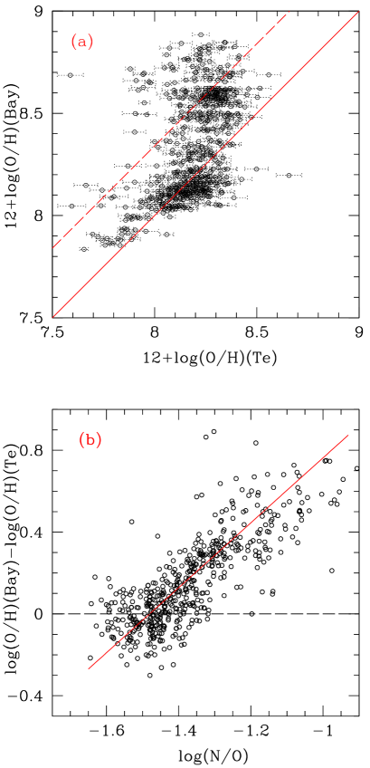
Figure 2: (a) Comparison between the electron temperature-based oxygen abundances and those Bayesian estimates obtained by the MPA/JHU group. The solid line is the equal-value line, and the long-dashed line represents a +0.34 dex discrepancy from the equal-value line to show the overestimates of the oxygen abundances by using the model of Charlot et al. (2006) for almost half of the sample galaxies. (b) The offset between the log(O/H)_Bay and the log(O/H)${}_{T_{e}}$ as a function of the log(N/O) abundance ratios for the MPA/JHU sample galaxies. The solid line is the linear least squares fit for the relations, given as Eq. (7).

4.2 $R_{23}$ method

Pagel et al.(1979) first proposed the empirical abundance indicator $R_{23}$ for metal-rich galaxies. Skillman et al. (1989) further suggested that this indicator also can be used for metal-poor galaxies. The relationship between O/H and $R_{23}$ has been extensively discussed in literature (see Tremonti et al. (2004) and references therein). Different calibrations will result in slightly different oxygen abundances even for the same branch (see fig. 3 of Tremonti et al. 2004 for comparison). A few calibrations have attempted to improve the calibration by introducing an empirical estimator of the ionization parameter as a second parameter (e.g. McGaugh 1991; Charlot & Longhetti 2001; KD02 etc.). At present, one of the popular formulas is the calibration given by Kobulnicky et al.(1999), which includes two analytical formulas, for the metal-rich and metal-poor branches respectively, and is derived from the photoionization model of McGaugh (1991).

As we mentioned in the introduction, $R_{23}$ may overestimate the actual O/H abundances by a factor of $\sim$0.2-0.5 dex (Kennicutt et al. 2003 etc.). On the basis of this large sample of 695 galaxies, here we compare their oxygen abundances derived from $R_{23}$ and $T_{e}$ methods. Figs. 3a,3b show this comparison, where we use the calibration formula of Kobulnicky et al. (1999) to derive the 12+log(O/H)${}_{R_{23}}$ for the sample galaxies. In Fig. 3a, for the galaxies with 12+log(O/H)${}_{T_{e}}$$<$7.95, we use their calibration formula for metal-poor galaxies; and for the galaxies with 12+log(O/H)${}_{T_{e}}$$\geq$8.2, we use their formulas for metal-rich branch. These two metallicity limits are defined following the $R_{23}-P$ method in Sect. 4.3 and some other related studies (Pilyugin 2000, 2001a,b; Shi et al. 2006). Fig. 3a shows that $R_{23}$ method will overestimate the O/H abundances by a factor of $\sim$0.20 dex, which is analogous to what was found by Kennicutt et al. (2003) and Shi et al. (2005, 2006). Detailed discussions about this discrepancy can be found in Kennicutt et al. (2003). For the sample galaxies with 8.0$<$12+log(O/H)${}_{T_{e}}$$<$8.2, which are in the turn-over region, the calibration of Kobulnicky et al. (1999) of metal-poor branch gives (O/H)${}_{R_{23}}$ in good agreement with (O/H)${}_{T_{e}}$. These galaxies are omitted when we discuss the discrepancy between the $T_{e}$- and $R_{23}$-based metallicities, which is acceptable. Fig. 3a does not show any obvious offset between the H ii regions and galaxies. Pérez-Montero & Díaz (2005) showed that the giant extragalactic H ii regions (GEHRs) have more dispersion than the H ii galaxies and H ii regions in the Galaxy and the Magellanic Clouds (their figs.1,3,7) since the GEHRs may have different ionizaiton parameters and stellar effective temperatures.

To illustrate clearly the uncertainties due to the double-valuedness of the $R_{23}$-O/H relation, we used both of the calibration formulas for metal-poor and metal-rich branches to calculate the 12+log(O/H)${}_{R_{23}}$ abundances for the galaxies having 7.9$<$12+log(O/H)${}_{T_{e}}$$<$8.4. Fig. 3b gives the results as the points between the two vertical dashed lines, which shows that these two different formulas will result in quite different metallicities, and the discrepancy may be up to $\sim$ 0.4 dex. Therefore, one should be very careful when using $R_{23}$-method to derive the metallicities of the galaxies having metallicities in the turn-over region.

4.3 The $R_{23}-P$ method

Pilyugin (2000, 2001a,b) suggested the $P$ method to estimate oxygen abundances of galaxies, in which the oxygen abundance can be derived from two parameters, $R_{23}$ and $P$ (=[O iii]/([O ii]+[O iii])). Therefore, we call this method as the “$R_{23}-P$ method”. They derived the O/H=$f(R_{23},P)$ formulas from a sample of metal-poor H ii regions with 7.1$<$12+log(O/H)${}_{T_{e}}$$<$7.95 and a sample of moderately metal-rich H ii regions with 8.2$<$12+log(O/H)${}_{T_{e}}$$<$8.7. The best fitting relation for metal-poor objects was given as Eq.(4) in Pilyugin (2000), and that for moderately metal-rich objects was given as Eq.(8) in Pilyugin (2001a).

Fig. 3c shows that there is slight difference of $\sim$0.06 dex between the $(O/H)_{T_{e}}$ and the $(O/H)_{R_{23}-P}$ abundances for the samples. Indeed, the good agreement is not surprising since Pilyugin (2000, 2001a,b) derived the $R_{23}-P$ method formulas by using a subset of the sample we use here (Izotov et al. 1994, 1997a and Izotov & Thuan 1998b,1999b). The minor offset is likely caused by two reasons: (1) our sample is much larger than that used by Pilyugin which allows us to determine the relations with higher precision; (2) the different $T_{e}$-formulas and/or atomic data used in calculations. Moreover, for the low excitation samples in low-metallicity branch with $P<$0.75, the $R_{23}-P$ method may overpredict their oxygen abundances by a factor $\sim$0.1 dex, which is consistent with the 0.1-0.2 dex overestimates found by van Zee & Haynes (2006) for the low excitation H ii regions in dwarf irregular galaxies.

Pilyugin & Thuran (2005) have renewed the $R_{23}-P$ calibrations by including several improvements, such as enlarging the sample by 1 order of magnitude etc. We have used the new calibrations to re-calculate the (O/H)${}_{R_{23}-P}$ abundances for our sample galaxies, and found the overestimate factor by the $R_{23}-P$ method decreases to be $\sim$0.025 dex.

Because there is no observational samples with 7.95$<$ 12+log(O/H)$<$ 8.2 in Pilyugin’s calibration for $R_{23}-P$ method, the $R_{23}-P$ method cannot provide information for the galaxies within this oxygen abundance range. To understand more about this, we calculate oxygen abundances for galaxies with 12+log(O/H)${}_{T_{e}}$=7.9–8.4 using the two formulas for the metal-rich and metal-poor branches. The results are indicated as the points between the two vertical dashed lines in Fig. 3d. Similarly to what we saw for $R_{23}$ the two branch calibrations give quite different metallicities with a difference of up to $\sim$0.4 dex. Thus one must be very careful when applying the $R_{23}-P$ method to samples of galaxies with metallicities in the turn-over region.

4.4 $N$2 method

The [N ii]/H$\alpha$ emission-line ratio can also be used to estimate metallicities of galaxies. Nitrogen is mainly synthesized in intermediate- and low-mass stars. The [N ii]/H$\alpha$ ratio will therefore become stronger with on-going star formation and evolution of galaxies, until very high metallicities are reached, i.e. 12+log(O/H)$>$9.0, where [N ii] starts to become weaker due to the very low electron temperature caused from strong cooling by metal ions. It is worth pointing out that this ratio gives an indirect measurement of the oxygen abundance however, since oxygen lines are not used in the method.

Following the earlier work by Storchi-Bergmann, Calzetti & Kinney(1994) and Raimann et al.(2000), D02 and PP04 suggested calibration relations for O/H vs. N2 index from 236 and 137 galaxies respectively. D02 combined a sample of 128 metal-rich galaxies and 108 metal-poor galaxies with [O iii]4363 detected to derive their calibration. The way they estimated the metallicities of their galaxy sample was to use the $T_{e}$-method for the metal-poor galaxies and the $R_{23}$ or $S_{23}$ (=log(([S ii]6717,6731+[S iii]9096,9531))/H$\beta$) method for the metal-rich ones. PP04 extracted the metal-poor objects from the work of D02 and updated the abundances for some of them with recent measurements by Kennicutt et al. (2003) for H ii regions in M101 and by Skillman et al. (2003) for dwarf irregular galaxies in the Sculptor Group. To be consistent with the $T_{e}$-method, here we use the calibration formula given by PP04 to derive the metallicities 12+log(O/H)_N2 for our 695 sample galaxies. Fig. 3e gives the comparison between the 12+log(O/H)${}_{T_{e}}$ and 12+log(O/H)_N2, which shows that the two estimates are consistent but with some scatter. The scatter may mostly come from the different ionization parameters of the galaxies, and the different samples (see Sect.6.5).

One of the advantages of using the N2 index for estimating metallicity is that the $N$2 indicator can break the degeneracy when the $R_{23}$-(O/H) and ($R_{23},P$) -(O/H) relations are double-valued. Also, the N2 index is not affected by dust extinction since H$\alpha$ and [N ii] are so closely spaced in wavelength. Furthermore near infrared spectrographs can measure these two lines for galaxies out to high redshifts, where equivalently to early epochs in the evolution of galaxies (see more discussion in Liang et al. 2006).

4.5 $O$3$N$2 method

$O$3$N$2 = log{([O iii]$\lambda 5007$/H$\beta$)/([N ii]$\lambda 6583$/H$\alpha$)} is another indicator for metallicities of galaxies. It was introduced by Alloin et al.(1979) and further studied by PP04. PP04 presented one such calibration by doing linear least squares fit for a sample of 65 (from the 137) galaxies with $-1<O3N2<$ 1.9, and provided a calibration formula. This calibration does not work for the cases of $O$3$N$2 $>1.9$ since the data points are so scattered there in their study. Fig. 3f shows the comparison between the 12+log(O/H)${}_{T_{e}}$ and the oxygen abundances derived from O3N2 method using the calibration of PP04 for our 695 sample galaxies. But we extrapolate to use the PP04’s calibration to the galaxies with $O3N2$$>$1.9.

It is clear that this calibration will overestimate the O/H abundances by a big factor, up to 1.0 dex, for the metal-poor galaxies with $O$3$N$2 $>$ 1.9 (about 12+log(O/H)$<$8.0). The scatter of the data with $-1<$$O$3$N$2 $<$ 1.9 are also large, which may be due to the different ionization parameters of the galaxies.

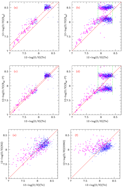
Figure 3: Comparison between the $T_{e}$-based abundances with those derived from other strong-line calibrations: (a,b). $R_{23}$ method; (c,d). $R_{23}-P$ method; (e). $N2$ method; (f). $O3N2$ method (see text). The small blue points represent the SDSS sample, and the larger magenta points (open circles) represent the sample compiled from literature. The solid lines are the equal-value lines, and the long-dashed lines in (a) and (c) are the linear least-squares fits to the data points, which show a discrepancy of $\sim$0.20 dex and $\sim$0.06 dex from the equal-value lines, respectively. The two pairs of vertical dashed lines in (b) and (d) show the range of 7.9$<$12+log(O/H)${}_{T_{e}}$$<$8.4 for the samples whose metallicities are estimated from strong-line ratios by using two calibrations for metal-rich and metal-poor branches.

5 Comparisons with photoionization models

KD02 has calculated the metallicity calibrations for strong-line ratios on the basis of photoionization models. They used a combination of stellar population synthesis and photoionization models to develop a set of ionization parameters and abundance diagnostics based on emission-line ratios from strong optical lines, with seven ionization parameters q = 5 $\times$ $10^{6}$, 1 $\times$ $10^{7}$, 2 $\times$ $10^{7}$, 4 $\times$ $10^{7}$, 8 $\times$ $10^{7}$, 1.5 $\times$ $10^{8}$, and 3 $\times$ $10^{8}$ cm s^-1. The ionization parameter $q$ is defined on the inner boundary of the nebula, and can be physically interpreted as the maximum velocity of an ionization front that can be driven by the local radiation field. It will be interesting to compare the observational samples with these model results. Fig. 4 shows the comparisons for the relations of 12+log(O/H) versus $R_{23}$, N2, O3N2 and S2 indices. These relations are for the $T_{e}$-based oxygen abundances of the metal-poor galaxies. Liang et al. (2006) has shown such relations for the metal-rich SDSS galaxies based on $R_{23}$ abundances, and derived the corresponding calibrations (see the thick solid lines in Figs. 4b,c).

Fig. 4a shows that the significant discrepancy in the theoretically expected $R_{23}$ sequence with respect to the observed trend beginning from 12 + log(O/H)${}_{T_{e}}=8.0$ to lower metallicities. Nagao et al. (2006) also pointed out this. The observed relation of $R_{23}$ - log(O/H) of the data points does not show much scatter in contrast to the models of the lower-branch of metallicity, which may mean the weak independence of $R_{23}$ on ionization parameters there. Especially, the distribution of observational data is nearly vertical in oxygen abundance range of $7.9\sim 8.5$. The physical reason for the insensitivity of $R_{23}$ to metallicity in this metallicity region is that the [O iii]/H$\beta$ ratio (also [O ii]/H$\beta$) is independent of $T_{e}$, hence of metallicity there (Stasinska 2002). It proves again that the oxygen abundance cannot be accurately measured by using $R_{23}$ in the metallicity turnover region, but $R_{23}$ indicator works well for the metal-poor galaxies with 12 + log(O/H)$<$7.9.

Fig. 4b shows the comparison between 12+log(O/H) and N2 index. It shows that the observational data follow the general trend of the model results well, namely, the N2 indices of galaxies increase following the increasing metallicities, up to 12+log(O/H)=9.0 (by models and Liang et al. 2006). The observational data show some scatter, which may be due to their different ionization parameters. We also plot a thick solid line (the short one) in Fig. 4b to show the calibration relation derived by Liang et al. (2006) with the metal-rich SDSS galaxies (8.5$<$12 + log(O/H)$<$9.3). If we derive a calibration from the $T_{e}$-based oxygen abundances of the metal-poor galaxies, and extrapolate it to the metal-rich region, it will result in relatively lower O/H abundance than directly using the calibration from metal-rich galaxies. Perhaps one reason for this discrepancy is from the different methods to determine metallicities of the metal-poor and metal-rich galaxies, i.e. the $T_{e}$-method versus the $R_{23}$-method or photoionization models. However, Stasińska (2005) pointed out that, at high metallicity, the derived O/H values from $T_{e}$ for model H ii regions deviate strongly from the true ones, i.e., important deviations appear around 12 + log(O/H)=8.6, and may become huge as the metallicity increases (see their fig.1a).

Fig. 4c shows the comparison between 12+log(O/H) and the O3N2 index. The general trend of the observations and that of the models are similar, and show increasing O/H abundance with decreasing O3N2 index. However, the large scatter of the data points in this plot may be due to the strong effect of ionization parameter, and such effect is stronger in the low-metallicity region (12+log(O/H)$<$8.5) than in the high-metallicity region (12+log(O/H)$>$8.5). Moreover, O3N2 is much less dependent on metallicity in the low-metallicity region than in the high-metallicity region, in particular, it is almost independent of metallicity for the sample galaxies with metallicities of 12+log(O/H)=7.1-7.7. This is possibly the main reason that PP04 had to limit their calibration to O3N2$<$1.9. We also present the calibration for metal-rich SDSS galaxies obtained by Liang et al. (2006) in Fig. 4c, which is given as the thick solid line (the short one) in the 8.5$<$12+log(O/H)$<$9.3 region. Both the calibrations for the metal-rich and metal-poor sample galaxies are consistent with the general trend of the model predictions, but the calibration for metal-poor galaxies corresponds to relatively higher ionization parameter than the metal-rich galaxies.

Fig. 4d shows the comparison between 12+log(O/H) and the S2 index. Both the observations and models clearly show an increasing S2 with increasing O/H. This increasing trend will extend up to 12+log(O/H)$\sim$8.9-9.0. S2 is affected more by the ionization parameters than the N2 index is. The large scatter of this relation may be caused by the different ionization parameters. Most of the SDSS galaxies cluster around $-1.0<S2<-0.5$. Liang et al. (2006) did not derive a metallicity calibration for S2 for the metal-rich galaxies since the data points show obvious turnover and double-valued distribution around 12+log(O/H)$\sim$8.9-9.0.

In summary, Figs. 4a-d show that $R_{23}$ is not a good metallicity indicator for the galaxies with 7.9$<$12+log(O/H)$<8.5$ due to its independence on metallicity there, and is a good indicator for lower metallicity region with 12+log(O/H)$<7.9$; N2 is a useful indicator for estimating metallicities of galaxies because it is strongly monotonicly correlated with metallicity (up to about 12+log(O/H)$\sim$9.0); although O3N2 and S2 can be used to estimate metallicities of galaxies, they are more sensitive to ionization parameters than N2 is, and O3N2 is less dependent on metallicity than the other two. In addition, when we have the indicator of O3N2 and/or S2, normally we also have N2. Furthermore, if we can find a way to take into account the ionization parameters of the sample galaxies in the calibrations, it will provide more reliable metallicities (see Sects. 6.5,6.6).

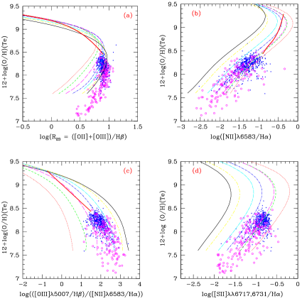
Figure 4: Comparison between the observational data and the photoionization models of KD02. The symbols are the same as in Fig. 3. The seven lines represent the model results from KD02 with seven photoionization parameters from q = 5 $\times$ $10^{6}$ cm s^-1 to q = 3 $\times$ $10^{8}$ cm s^-1, which increase orderly from the red dotted line to the black solid line. The solid thick line (in red) in Fig.(a) is the calibration derived by Tremonti et al. (2004) for the metal-rich galaxies, and those in Fig.(b) and Fig.(c) are the calibrations derived by Liang et al. (2006) for the metal-rich SDSS galaxies.

6 Deriving oxygen abundance calibrations

We have obtained the $T_{e}$-based O/H abundances for the 695 sample galaxies and H ii region. They have metallicities of $7.1<$12+log(O/H)${}_{T_{e}}$ $<8.5$ mostly. Then we use their (O/H)${}_{T_{e}}$ and line ratios to re-derive the oxygen abundance calibrations for the strong-line ratios N2, O3N2 indices, and add a S2 index. We also derive the calibration for $R_{23}$ for the 12+log(O/H)${}_{T_{e}}$ $<7.9$ region. Moreover, we try to add an excitation parameter $P$ (=[O iii]/([O ii]+[O iii])) in the calibrations to separate the sample galaxies to be three sub-samples, which improves the N2 calibration, but does not improve well the O3N2 and S2 calibrations.

6.1 The $R_{23}$ index

The $R_{23}$ index is useful for calibrating metallicities of low metallicity galaxies with 12+log(O/H)$<$7.9 due to its obvious correlation with log(O/H) and weak dependence on ionization parameters there. Fig. 5a shows this correlation. The linear least-squares fit for all the 120 data points with 12+log(O/H)$<$7.9 is:

$$12+\rm log(O/H)=6.486+1.401\times log(R_{23}),$$ (8)

with $R_{23}$=([O ii]$\lambda$3727+ [O iii]$\lambda$$\lambda$4959,5007)/H$\beta$. The rms of the data to the fit is about 0.103 dex. The appropriate range of this calibration is about 0.4$<$log($R_{23}$)$<$1.0 and 7.0$<$12+log(O/H)$<$7.9. The calibrations of Kobulnicky et al.(1999) are also presented in the figure for comparison as the dashed lines for the cases of $y$ (=log([O iii]/[O ii])) equal to 0, 1, 1.5. It shows that the $y$=1.0 and 1.5 can explain these observational data generally.

6.2 The N2 index

Since the data points show a relatively tight linear relationship between $N$2 and 12+log(O/H), we obtain a linear least-squares fit for this relation. We use the mean-value points in 11 bins of metallicities to avoid too much weights on the high metallicity range where most of the data are distributed. The bin width is $\Delta$[log(O/H)] = 0.1 for the galaxies in the range of $7.4<$12+log(O/H) $<8.5$, and $\Delta$[log(O/H)] = 0.3 for the range of 7.1 $<$ 12 + log(O/H)${}_{T_{e}}$ $<$ 7.4 because of the small number of sources in this range. These bin widths are the same as for the O3N2 and S2 indices discussed in the consequent two subsections. The objects with higher uncertainty than 0.06 dex on log(O/H) and log([N ii]/H$\alpha$) have been excluded in calculating the mean values and calibrating, which leaves 584 data points. 19 galaxies from literature cannot be included in deriving calibrations since they do not have [N ii] emission-line measurements. The derived analytical relation of a linear least squares fit is:

$$12+\rm log(O/H)=9.263+0.836\times N2,$$ (9)

with $N$2=log([N ii]$\lambda$6583/H$\alpha$), shown as the solid line in Fig. 5b. The rms of the data to the fit is 0.159 dex. The two dashed lines show a spread of 2$\sigma$. This calibration is valid in the range of $-2.5<N2<-0.5$. The calibrations of D02 ($12+\log{\rm(O/H)}=9.12+0.73\times N2$, the dotted line) and PP04 ($12+\log{\rm(O/H)}=8.90+0.57\times N2$, the long-dashed line) are also plotted for comparison. It shows that D02’s calibration is similar to ours, but the one of PP04 shows a slightly lower slope and the difference is more obvious for the low metallicity region with 12+log(O/H)$<$8.0. The reason may be that PP04’s sample does not extend to much lower metallicity with 12+log(O/H)$<$7.7, and most of their samples have metallicities of 7.7$<$12+log(O/H)$<$8.5, while the fit for their these samples results in a bit lower slope than for ours (see fig.1 of D02 and fig.1 of PP04).

6.3 The O3N2 index

Fig. 5c shows our sample galaxies for their (O/H)${}_{T_{e}}$ abundances versus O3N2 indices. Although they are quite scattered, there still exists an obvious trend, i.e., O/H increases following the decreasing O3N2 index. We try to derive a calibration of O3N2 index for O/H abundances from these sample galaxies. The objects with an higher uncertainty than 0.06 dex on log(O/H) and O3N2 are excluded, which leaves 585 data points. 19 objects from literature without their [N ii] emission-line measurements are excluded. The mean-value points within 11 bins are obtained for the left sample galaxies. The bin widths are the same as for the N2 calibration (Sect. 6.2). A two-order polynomial fit is obtained by fitting the mean-value points:

$$12+\rm log(O/H)=8.203+0.630\times O3N2-0.327\times O3N2^{2},$$ (10)

with O3N2 = log[([O iii]$\lambda$5007/H$\beta$)/([N ii]$\lambda$6583/H$\alpha$)], shown as the solid line in Fig. 5c. The rms of the data to the fit is 0.199 dex. This fit is valid for 1.4$<$O3N2$<$3. The two dashed lines show 2$\sigma$ discrepancy. The calibration of PP04 ($12+\rm{log(O/H)}=8.73-0.32\times O3N2$) has been plotted as the long-dashed line, which is only valid for 1$<$O3N2$<$1.9. The calibration of PP04 shows a shallower slope than ours, which comes from their much smaller sample (65 objects) and the much narrower O3N2 range.

6.4 The S2 index

S2 = log([S ii]$\lambda\lambda$6717,6731/H$\alpha$) is also a metallicity-sensitive indicator. Although it is less useful than N2 for metallicity calibration due to the stronger dependence on ionization parameter, it is still interesting to derive a calibration from S2 since it is dependent on metallicity monotonicly in the studied metallicity range. This relation has the advantage of not being strongly dependent on reddening corrections. Although the sample data is much scatter, a linear relation exists obviously between O/H and S2.

We calculated the mean values of S2 and O/H abundances for the sample galaxies in 11 bins, the bin widths are the same as we used for the N2 and O3N2 calibrations. Again, the objects with an higher uncertainty than 0.06 dex on log(O/H) and log([S ii]/H$\alpha$) are excluded in the calculations, which leaves 607 data points. A least-squares linear fit to the mean-valued points yields the relation:

$$12+{\rm log(O/H)}=9.128+1.051\times S2,$$ (11)

with S2 = log([S ii]$\lambda\lambda$6717,6731/H$\alpha$), which is shown by the solid line in Fig. 5d. The rms of the data to the fit is about 0.176 dex. The two dashed lines show the discrepancy of 2$\sigma$.

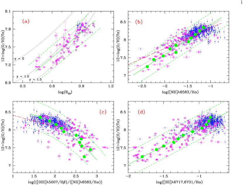
Figure 5: $R_{23}$, N2, O3N2 and S2 indices for oxygen abundance calibrations from the sample galaxies: (a). the $R_{23}$ index; (b). the N2 index; (c). the O3N2 index; (d). the S2 index. The small filled points represent the SDSS galaxies and the open squares refer to the samples from literature. The points with uncertainties larger than 0.06 dex in all these line ratios and log(O/H) abundances have been excluded. The solid line in Fig.(a) refers the linear least-squares fit for all the 120 data points in the figure. The three dashed lines refer the calibrations given by Kobulnicky et al. (1999) for the three different cases of $y$ (=log([O iii]/[O ii])). In Fig.(b), the long-dashed and dotted lines refer to the calibrations of PP04 and D02, respectively. In Fig.(c), the long-dashed line refers to the calibration of PP04. In Figs.(b-d), the 11 large filled circles represent the mean values in each bin of oxygen abundances (see text), and the solid lines are the least-squares fits for these mean-value points. The two dashed lines show the 2$\sigma$ discrepancy from the fits in all the four panels.

6.5 Add the P parameter

The calibration of O/H vs. N2 is dependent on ionization parameter (Fig. 4b), as well the O3N2 and S2 indices (Figs. 4c,d). Therefore, to get more reliable O/H abundances, an excitation parameter could be included in the calibrations which correlates strongly with ionization parameter and the hardness of the ionizing radiation field. We use the $P$ parameter given by Pilyugin (2000, 2001a,b), where $P$ was defined as [O iii]/([O ii]+[O iii]), which is similar to [O iii]/[O ii], the excitation parameter used by Kobulnicky et al. (1999) in calibrations. We should notice that $P$ needs to be computed from the dereddened emission lines.

In Fig. 6a, we plot the (log(O/H)${}_{T_{e}}$ - log(O/H)_N2) vs. $P$ relations for the sample galaxies, which shows that these galaxies can roughly be separated to be three subsamples with $P<$0.65 (143 data points), 0.65$<P$$<$0.80 (292 data points) and $P>0.80$ (149 data points). We derive the N2 calibrations for these three subsamples individually. The analytical calibrations of linear least-squares fits for the three subsamples with different $P$ parameters are:

$$12+\rm log(O/H) = 9.514+0.916\times N2,\leavevmode\nobreak\ \leavevmode\nobreak\ \leavevmode\nobreak\ (P>0.80),$$ (12)

$$= 9.457+0.976\times N2,\leavevmode\nobreak\ \leavevmode\nobreak\ \leavevmode\nobreak\ (0.65<P<0.80),$$

$$= 9.332+0.998\times N2,\leavevmode\nobreak\ \leavevmode\nobreak\ \leavevmode\nobreak\ (P<0.65),$$

which are given as the solid, long-dashed and dashed lines in Fig. 6b, respectively. The rms of the data to each fit are 0.150, 0.140, 0.189 dex, respectively. The dotted lines are the photoionization model results of KD02. It shows that the three different $P$ values just correspond to the cases of KD02 of $q=4\times 10^{7}$, $1\times 10^{7}$(as well $2\times 10^{7}$) and $5\times 10^{6}$ cm s^-1, respectively.

We have also tried to add $P$ as an additional parameter for the O3N2 and S2 indices. The sample galaxies are separated into three sub-samples with $P$$<$0.60, 0.60$<$$P$$<$0.85 and $P$$>$0.85 to derive calibrations for these two indices. The basic results follow the photoionization models of KD02 consistently. However, we find adding a $P$ parameter does not improve the fits much. Therefore, we won’t present the two-parameter calibrations for the O3N2 and S2 indices as figures here. We should notice that using $P$ with [N ii]/H$\alpha$ means that we need observations covering a much wider wavelength range, which might not be practical at high $z$. It is not necessary to add the $P$ parameter to the $R_{23}$ calibration since the observational data in the $R_{23}$ vs. O/H relation does not show obvious dependence on ionization parameter in contrast to the lower-branch models (Fig. 4a).

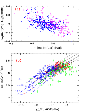
Figure 6: (a). The relation between log(O/H)${}_{T_{e}}$-log(O/H)_N2 vs. $P$ for the sample galaxies, which shows that they can be roughly divided into three subsamples with different $P$ parameters: $P>0.80$, $0.65<P<0.80$ and $P<0.65$. The symbols are the same as in Fig. 4. (b). The calibration of N2 index together with the $P$ parameter. The blue open squares represent the samples with $P>0.80$, the red points represent those with $0.65<P<0.80$, and the green triangles represent those with $P<0.65$. The solid, long-dashed and short-dashed lines refer to the linear least-squares fits for each of the three subsamples, respectively (Eq. (12)). The five dotted lines are the model results of KD02, from the right to the left ones, the ionization parameter $q$ increases from the 5$\times 10^{6}$ to the 1$\times 10^{7}$, 2$\times 10^{7}$, 4$\times 10^{7}$ and 8$\times 10^{7}$ cm s^-1 grids.

6.6 The accuracies of the derived calibrations

We have presented the least-squares fits for the relations of 12 + log(O/H)${}_{T_{e}}$ and $N$2, $O$3$N$2 and $S$2 indices with and without considering the $P$ excitation parameter. To show the accuracies of these calibrations, we plot in Figs. 7a-d the comparisons between log(O/H)${}_{T_{e}}$ and those from line indices. Figs. 7a,c,d show the comparisons with the calibrated abundances from N2, O3N2, S2 indices following Eqs. (9-11), which have been given as the solid lines in Figs. 5b-d, respectively. Fig. 7b show the calibrated abundances from the N2 index but adding the $P$ parameter following Eq. (12). Adding the $P$ parameter has improved the N2 calibration. Among these, the rms of the O3N2 and S2 calibrations are large, about 0.191 and 0.171 dex respectively (Fig. 7c,d). The calibration of (N2,$P$) case (Fig. 7b) shows the lowest rms, which is about 0.158, a bit lower than the rms in Fig. 7a and Fig. 3e for the N2 calibration (0.162 and 0.160 dex respectively).

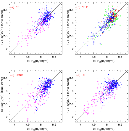
Figure 7: Comparisons between the $T_{e}$-based O/H abundances with those derived from strong-line ratios, including N2 (without and with $P$), O3N2 and S2 indices: (a). for the N2 index (without $P$, Eq.(9), Fig. 5b); (b). for the N2 index (with $P$, Eq.(12), Fig. 6); (c). for the O3N2 index (Eq.(10), Fig. 5c); (d). for the S2 index (Eq.(11), Fig. 5d). The rms values of the data to the equal-value lines in each plot are 0.162, 0.158, 0.191 and 0.171 dex, respectively, they will increase to be 0.173, 0.167, 0.215 and 0.203 dex if the data points with uncertainties larger than 0.06 dex in line indices and log(O/H) are included. The symbols in Figs.(a,c,d) are the same as in Fig. 4, and the symbols in Fig.(b) are the same as in Fig. 6b.

Some of the remaining scatter in log(O/H)_N2,P may come from the different star forming history and evolutionary status of the sample galaxies. Fig. 8 shows a clear correlation between the log(O/H)_N2,P - log(O/H)${}_{T_{e}}$ and the log(N/O) abundance ratios of the sample galaxies, which can be given as a linear least squares fit:

$$\rm log(O/H)_{N2,P}-log(O/H)_{T_{e}}=0.902\times log(N/O)+1.240,$$ (13)

with a rms of 0.104 dex. The corrected calibration of (N2,P) by considering this correlation will provide much accurate oxygen abundance, and the rms of the data to the equal-value lines in Fig. 7a and Fig. 7b will decrease to be 0.115 dex, which is much less than the previous ones (0.162 and 0.158 dex, respectively). This correlation can be used to correct the derived oxygen abundances from strong-line ratio when it is necessary. Nevertheless, to apply the N/O correction to 12+log(O/H) abundances, we need to measure [O ii], [O iii] and H$\beta$ in addition to [N ii] and H$\alpha$, thus it will not always be practical.

We should notice that both the $x$ and $y$ axis of Fig. 8 depends on nitrogen abundance, which means that the observed correlation could be spurious if the errors in log(N) are large. However, the errors of the log(N/O) abundances of the sample galaxies are quite small. It is about 0.011 dex on average for the MPA/JHU sample galaxies, which is expected since we only select the objects with higher signal-to-noise ratio, i.e. larger than 5$\sigma$, on the flux measurements of [N ii] (see Sect.2.1). For other samples from literature, the errors of their log(N/O) values are about 0.021 dex on average. Therefore, this correlation is robustly measured, and could be used to correct 12+log(O/H)_N2,P measurements if desired. More importantly, the strong trend in Fig. 8 highlights the sensitivity of the N2 calibration to a galaxy’s past history of star formation, since it determines the present-day N/O ratio.

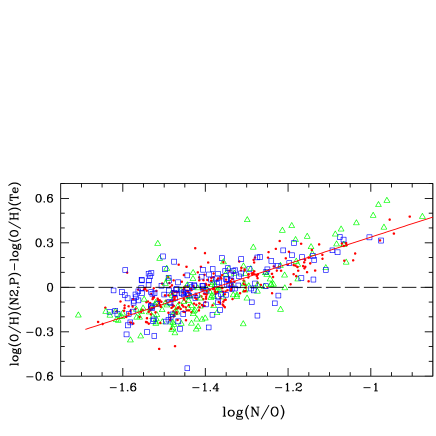
Figure 8: Correlation between the difference of log(O/H)_N2,P and log(O/H)${}_{T_{e}}$ and the log(N/O) abundance ratios of the sample galaxies. The symbols are the same as in Figs. 6b,7b. The solid line is the linear least squares fit for the relations with a rms of 0.104 dex.

7 Conclusions

We compiled a large sample of 695 low-metallicity galaxies and H ii regions with [O iii]4363 detected, which consists of 531 galaxies from the SDSS-DR4 and 164 galaxies and H ii regions from literature. We determined their electron temperatures, electron densities, and then the $T_{e}$-based oxygen abundances. The derived oxygen abundances of them are 7.1$<$12+log(O/H)$<$8.5.

The comparison between the $T_{e}$-based oxygen abundances and the Bayesian metallicities obtained by the MPA/JHU group show that, for about half of the MPA/JHU sample galaxies in this study, their O/H abundances were overestimated by a factor of 0.34 dex on average by using the photoionization models (Charlot et al. 2006; Tremonti et al. 2004; Brinchmann et al. 2004). This is possibly related to how secondary nitrogen enrichment is treated in the models they used.

The $T_{e}$-derived oxygen abundances of these sample galaxies were compared with those derived from other strong-line ratios, such as $R_{23}$, $R_{23}-P$, $N$2 and $O$3$N$2 indicators. The results show that $R_{23}$ and $R_{23}-P$ methods will generally overestimate the oxygen abundances of the sample galaxies by a factor of $\sim$0.20 dex and $\sim$0.06 dex, respectively. This 0.06 dex discrepancy is quite small, and will decrease to be 0.025 dex when the improved $R_{23}-P$ calibrations given by Pilyugin & Thuan (2005) are used. The abundance calibration of N2 index, rather than O3N2 index, from PP04 can result in consistent O/H abundances with (O/H)${}_{T_{e}}$ but with a scatter of about 0.16 dex.

From this large sample of 695 star-forming galaxies and H ii regions, we re-derive abundance calibrations for $R_{23}$, N2, O3N2 and S2 indices on the basis of their oxygen abundances derived from $T_{e}$. The N2, O3N2 and S2 indices monotonicly change following the increasing O/H abundances from 12+log(O/H)=7.1 to 8.5, which are consistent with the photoionization model results of KD02. $R_{23}$ is a good metallicity indicator for the metal-poor galaxies with 12+log(O/H)$<$7.9. Nevertheless, $R_{23}$ does not follow the KD02 models well.

The scatter of the observational data may come from the differences in the ionizing radiation field. We add an excitation parameter $P$ to separate the sample galaxies to be three sub-samples, and then re-derive the N2 calibrations with three different $P$ cases ($<$0.65, 0.65-0.80, $>$ 0.80), which improves the calibration, confirmed by the decreasing rms of the data to the equal-value line, which decreases from 0.162 in Fig. 7a to 0.158 in Fig. 7b. But adding the $P$ parameter in the O3N2 and S2 indices does not improve the calibrations. However, some of the remaining scatter in the (N2,P) calibration may come from the different star forming history and evolutionary status of the galaxies, which can be confirmed by the correlation between the log(O/H)_N2,P - log(O/H)${}_{T_{e}}$ and log(N/O) of them (Fig. 8 and Eq. 13).

In the future studies about calibrating oxygen abundances of galaxies, when their $T_{e}$ values are not available, we can use the $R_{23}$, N2, O3N2 or S2 indices, together with the $P$ parameter sometimes (if the wavelength coverage is wide enough), to calibrate their oxygen abundances. $R_{23}$ shows obvious correlation with oxygen abundances for the low-metallicity galaxies with 12+log(O/H)$<$7.9. Comparing with O3N2 and S2, N2 is less affected by ionization parameter and more obviously correlate with O/H abundances. Also it can be detected by the near infrared instruments for the intermediate- and high-$z$ star-forming galaxies. The N2 index has helped to provide important information on the metallicities of galaxies at high-$z$, for example, Shapley et al. (2004) for a sample of 7 star-forming galaxies at 2.1$<$$z$$<$2.5, Shapley et al. (2005) for a sample of 12 star-forming galaxies at $z\sim$1.0-1.5, and Erb et al. (2006) from the six composited spectra of 87 rest-frame UV-selected star-forming galaxies at $z$$>$2 etc. However, considering the dependence of N2 (as well the (N2,P)) calibration on log(N/O) shown as Fig. 8, we should keep in mind that the resulted log(O/H) abundances from N2 may involve the specific history of N-enrichment in the galaxies. We may worry a bit about comparing the low and high-$z$ observations using [N ii] for this reason.

Given the good consistency of our N2 and S2 abundance calibrations with the models of KD02 at low metallicity (see Fig. 4b,d), it may be appropriate to linearly extrapolate our calibrations up to the high metallicity region, up to 12+log(O/H)$\sim$9.0 and 8.8 respectively. However, this extrapolation on N2 will result in lower log(O/H) abundance than the one directly derived from the calibration of the metal-rich SDSS galaxies obtained by Liang et al. (2006), which may be due to the discrepancy between the $T_{e}$- and the $R_{23}$-based metallicities. However, the $T_{e}$-based O3N2 calibration cannot be directly extrapolated to the metal-rich region since the slopes of the correlation relations between log(O/H) vs. O3N2 are not the same in the high-metallicity branch as in the low-metallicity branch (Fig. 4c). $R_{23}$ parameter cannot provide reliable oxygen abundances for the galaxies in the metallicity turn-over region with 7.9$<$12+log(O/H)$<$8.5.

References

- (1) Adelman-McCarthy, J. K. et al., 2006, ApJS, 162, 3!8
- (2) Alloin, D., Collin-Souffrin, S., Joly M., Vigroux, L., 1979, A&A, 78, 200
- (3) Baldwin, J., Phillips, M.M., Terlevich, R.J., 1981, PASP, 93, 5
- (4) Bresolin, F., Garnett, D.R., & Kennicutt, R. C. Jr., 2004, ApJ, 615, 228
- (5) Bresolin, F., Schaerer, D. et al. 2005, A&A, 441, 981
- (6) Brinchmann, J., Charlot, S., White, S.D.M., Tremonti, C., Kauffmann, G., Heckman, T. & Brinkmann, J., 2004, MNRAS, 351, 1151
- (7) Bruzual, A.G., Charlot, S., 2003, MNRAS, 344, 1000
- (8) Calzetti, D., Kinney, A.L., Storchi-Bergmann, T., 1994, ApJ, 429, 582
- (9) Charlot, S. & Longhetti, M., 2001, MNRAS, 323, 887 (CL01)
- (10) de Robertis, M.M., Dufour, R. J., Hunt, R.W., 1987, JRASC, 81, 195
- (11) Denicoló, G., Terlevich, R., Terlevich, E., 2002, MNRAS, 330, 69 (D02)
- (12) Díaz, A.I., Pérez-Montero, E., Vílchez, J.M., Pagel, B.E., Edmunds, M.G., 1991, MNRAS, 253, 245
- (13) Erb, D. K., Shapley, A. E., Pettini, M. et al. 2006, ApJ, 644, 813
- (14) Garnett, D.R., 1992, AJ, 103, 1330
- (15) Garnett, D.R., Edmunds, M.G., Henry, R.B.C., Pagel, B.E.J., Skillman, E.D., 2004a, ApJ, 128, 2722
- (16) Garnett, D.R., Kennicutt, R.C. Jr., Bresolin, F., 2004b, ApJ, 607, L21
- (17) Guseva, N.G., Papaderos, P., Izotov, Y.I., et al. 2003a, A&A, 407, 75
- (18) Guseva, N.G., Papaderos, P., Izotov, Y.I., et al. 2003b, A&A, 407, 91
- (19) Guseva, N.G., Papaderos, P., Izotov, Y.I., et al. 2003c, A&A, 407, 105
- (20) Izotov, Y.I., Andrew, B.D., et al. 1996, ApJ, 458, 524
- (21) Izotov, Y.I., Chaffee, F.H., Foltz, R.F., Green, R.F., Guseva, N.G., Thuan, T.X., 1999a, ApJ, 527, 757
- (22) Izotov, Y.I., Chaffee, F.H., Green, R.B., 2001a, ApJ, 562, 727
- (23) Izotov, Y.I., Chaffee, F.H., Schaerer, D., 2001b, A&A, 378, L45
- (24) Izotov, Y.I., Lipovetsky, V.A., et al. 1997b, ApJ, 476, 698
- (25) Izotov, Y.I., Papaderos, P., Guseva, N.G., Fricke, K.J., Thuan, T.X., 2004b, A&A, 421, 539
- (26) Izotov, Y.I., Stasinska, G., Meynet, G., Guseva, N.G., Thuan, T.X., 2005, A&A, 448, 955
- (27) Izotov, Y.I., Thuan, T.X., 1998a, ApJ, 497, 227
- (28) Izotov, Y.I., Thuan, T.X., 1998b, ApJ, 500, 188
- (29) Izotov, Y.I., Thuan, T.X., 1999b, ApJ, 511, 639
- (30) Izotov, Y.I., Thuan, T.X., 2004a, ApJ, 602, 200
- (31) Izotov, Y.I., Thuan, T.X., Lipovetsky, V.A., 1994, ApJ, 435, 647
- (32) Izotov, Y.I., Thuan, T.X., Lipovetsky, V.A., 1997a, ApJS, 108, 1
- (33) Kauffmann, G., Heckman, T.M., Tremonti, C.A., et al. 2003, MNRAS, 346, 1055
- (34) Kennicutt, R.C.Jr., 1992, ApJ, 388, 310
- (35) Kennicutt, R.C.Jr., Bresolin, F., Garnett, D.R., 2003, ApJ, 591, 801
- (36) Kewley, L.J., & Dopita, M.A., 2002, ApJS, 142, 35 (KD02)
- (37) Kewley, L.J., Dopita M., Sutherland R., Heisler C., Trevena J., 2001, ApJ, 556, 121
- (38) Kewley, L.J., Jansen, R.A., Geller, M.J., 2005, PASP, 117, 227
- (39) Kinney, A.L., Bohlin, R.C., Calzetti, D., Panagia, N., Wyse, R.F.G., 1993, ApJS, 86, 5
- (40) Kniazev, A.Y., Pustilnik, S.A., Masegosa, J., et al. 2000, A&A, 357, 101
- (41) Kobulnicky, H.A., Kennicutt, R.C.Jr., & Pizagno, J.L., 1999, ApJ, 514, 544 (K99)
- (42) Lamareille, F., Contini, T., Brinchmann, J., Le Borgne, J.-F., Charlot, S., & Richard, J. 2006, A&A, 448, 907
- (43) Lee, J.C., Salzer, J.J., & Melbourne, J., 2004, ApJ, 616, 752
- (44) Liang, Y.C., Yin, S.Y., Hammer, F. et al. 2006, ApJ (in press), astro-ph/0607074
- (45) McGaugh, S. S. 1991, ApJ, 380, 140
- (46) Melbourne, J., Phillips, A., Salzer, J.J., Gronwall, C., Sarajedini, V.l., 2004, AJ, 127, 686
- (47) Moustakas, J. & Kennicutt, R.C.Jr. 2006, ApJ, astro-ph/0511731,
- (48) Nagao, T., Maiolino, R., Marconi, A., 2006, A&A, (in press), astro-ph/0603580
- (49) Osterbrock, D.E., 1989, Astrophysics of Gaseous Nebulae and Active Galactic Nuclei. Mill Valley, California: University Science Books
- (50) Pagel, B.E.J., Edmunds, M.G., Blackwell, D.E., et al. 1979, MNRAS, 189, 95
- (51) Pettini, M., & Pagel, B.E.J., 2004, MNRAS, 348, L59 (PP04)
- (52) Pérez-Montero, E., Díaz, A.I., 2005, MNRAS, 361, 1063
- (53) Pilyugin, L.S., 2000, A&A, 362, 325
- (54) Pilyugin, L.S., 2001a, A&A, 369, 594
- (55) Pilyugin, L.S., 2001b, A&A, 373, 56
- (56) Pilyugin, L. S., Contini, T., Vílchez, J. M., 2004, A&A, 423, 427
- (57) Pilyugin, L. S. Thuan, T. X., 2005, ApJ, 631, 231
- (58) Pilyugin, L. S. Thuan, T. X., Vílchez, J. M., 2006, MNRAS, 367, 1139
- (59) Raimann, D., Storchi-Bergmann, T., Bica, E., et al. 2000, MNRAS, 316, 559
- (60) Shapley, A. E., Coil, A. L., Ma, C. P., Bundy, K., 2005, ApJ, 635, 1006
- (61) Shapley, A. E., Erb, D. K., Pettini, M. et al. 2004, ApJ, 612, 108
- (62) Shaw, R.A., & Dufour, R.J., 1995, PASP, 107, 896
- (63) Shi, F., Kong, X., Li, C., Cheng, F.Z., 2005, A&A, 437, 849
- (64) Shi, F., Kong, X., Cheng, F.Z., 2006, A&A, 453, 487
- (65) Skillman, E.D., Cote, S., Miller, B. W., 2003, AJ, 125, 610
- (66) Skillman, E.D., Kennicutt, R.C.Jr., Hodge, P.W., 1989, ApJ, 347, 875
- (67) Stasińska, G. 2002, lectures to be published in the proceedings of the XIII Canary Islands Winter School of Astrophysics, astro-ph/0207500
- (68) Stasińska, G., & Leitherer C., 1996, ApJS, 107, 661
- (69) Stasińska, G. 2005, A&A, 434, 507
- (70) Storchi-Bergmann, T., Calzetti, D., Kinney, A.L., 1994, ApJ, 429, 572
- (71) Thurston, T. R., Edmunds, M. G., Henry, R. B. C. 1996, MNRAS, 283, 990
- (72) Tremonti, C.A., Heckman, T.M., Kauffmann, G., et al. 2004, ApJ, 613, 898
- (73) van Zee, L., 2000, ApJ, 543,L31
- (74) van Zee, L. & Haynes, M. P. 2006, ApJ, 636, 214
- (75) Veilleux, S., Osterbrock, D., 1987, ApJS, 63, 295
- (76) Vílchez, J.M., & Iglesias-Páramo, J., 2003, ApJS, 145, 225