The structure of the cometary globule CG 12: a high latitude star forming region

The structure of the high galactic latitude Cometary Globule 12 (CG 12) has been investigated by means of radio molecular line observations. Detailed, high signal to noise ratio maps in C¹⁸O (1–0), C¹⁸O (2–1) and molecules tracing high density gas, CS (3–2), $\mathrm{DCO^{+}}$ (2–1) and $\mathrm{H^{13}CO^{+}}$ (1–0), are presented. The C¹⁸O line emission is distributed in a $10\arcmin$ long North-South elongated lane with two strong maxima, CG 12-N(orth) and CG 12-S(outh). In CG 12-S the high density tracers delineate a compact core, $\mathrm{DCO^{+}}$ core, which is offset by 15″ from the $\mathrm{C^{18}O}$ maximum. The observed strong $\mathrm{C^{18}O}$ emission traces the surface of the $\mathrm{DCO^{+}}$ core or a separate, adjacent cloud component. The driving source of the collimated molecular outflow detected by White (1993) is located in the $\mathrm{DCO^{+}}$ core. The $\mathrm{C^{18}O}$ lines in CG 12-S have low intensity wings possibly caused by the outflow.The emission in high density tracers is weak in CG 12-N and especially the $\mathrm{H^{13}CO^{+}}$, $\mathrm{DCO^{+}}$ and $\mathrm{N_{2}H^{+}}$ lines are +0.5 $\mathrm{km\,s^{-1}}$  offset in velocity with respect to the $\mathrm{C^{18}O}$ lines. Evidence is presented that the molecular gas is highly depleted. The observed strong $\mathrm{C^{18}O}$ emission towards CG 12-N originates in the envelope of this depleted cloud component or in a separate entity seen in the same line of sight. The $\mathrm{C^{18}O}$ lines in CG 12 were analyzed using Positive Matrix Factorization, PMF. The shape and the spatial distribution of the individual PMF factors fitted separately to the $\mathrm{C^{18}O}$ (1–0) and (2–1) transitions were consistent with each other. The results indicate a complex velocity and line excitation structure in the cloud. Besides separate cloud velocity components the $\mathrm{C^{18}O}$ line shapes and intensities are influenced by excitation temperature variations caused by e.g, the molecular outflow or by molecular depletion. Assuming a distance of 630 pc the size of the CG 12 compact head, 1.1 pc by 1.8 pc, and the $\mathrm{C^{18}O}$ mass larger than 100 M_☉ are comparable to those of other nearby low/intermediate mass star formation regions.

1 Introduction

Herschel (1847) noted that a 10^th mag. star, now known as h4636 or CoD~–39°~8581, is a binary with a separation of 3$\aas@@fstack{\prime\prime}$7. In the optical, h4636 illuminates the bright reflection nebula NGC~5367. Hawarden & Brand (1976) showed that it lies in the head of an impressive Cometary Globule 12, CG~12, with a tail stretching about one degree to the SE. With a galactic latitude of 21° and at the distance of 630 pc estimated by Williams et al. (1977), CG 12 lies more than 200 pc above the plane. CG 12 has an associated low/intermediate mass stellar cluster which has at least 9 members (Williams et al. 1977). The clouds cometary structure could be due to the passage of a supernova blast wave. Curiously, the cometary tail stretches towards the Galactic plane which would place the putative supernova even farther away from the Galactic plane than the globule. According to Maheswar et al (1996) the head of CG 12 is pointing towards the centre of an HI shell. Such a shell is, however, not readily evident in the whole sky HI survey (Kalberla et al. (2005)) which merges the northern Leiden/Dwingeloo Survey (Hartman & Burton 1997 ) and the southern Instituto Argentino de Radioastronomia Survey (Arnal et al. (2000)). The CG 12 cloud cometary shape is also seen in the IRAS surface emission (Odenwald (1988)).

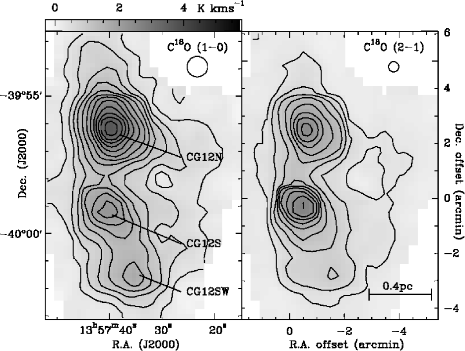
Figure 1: Maps of integrated emission of C¹⁸O (1–0) and C¹⁸O (2–1) $\int$$T_{A}^{*}$ dv from $-8$ $\mathrm{km\,s^{-1}}$ to $-4$ $\mathrm{km\,s^{-1}}$ in CG12. The lowest contour and the contour increment are 0.3 $\mathrm{K\,km\,s^{-1}}$. The SEST half power beam sizes are shown in the upper corners of the panels. Offsets from the map centre position, $13^{\mathrm{h}}57^{\mathrm{m}}43\aas@@fstack{s}1,-39\degr 58\arcmin 43\aas@@fstack{\prime\prime}3$ (J2000), are shown on the axes of the right panel. The scale tick in the lower right corner assumes a distance of 630 pc to the cloud.

White (1993) mapped the region around and south of h4636 in ¹²CO (2–1) and C¹⁸O (2–1) lines with a spatial resolution of 22″. He found a small size C¹⁸O core near the binary, and a molecular outflow with a centre close to the binary system. Further large scale $\mathrm{{}^{12}CO}$ , $\mathrm{{}^{13}CO}$ and $\mathrm{C^{18}O}$ observations with 2$\aas@@fstack{\prime}$7 resolution are presented in Yonekura et al. (1999). CG 12 contains two compact 1.2mm continuum sources, one in the direction of the $\mathrm{C^{18}O}$ core detected by White (1993) (Reipurth et al. 1996) and another one two arcminutes north of it (Haikala 2006, in preparation). The centres of the continuum sources were observed in $\mathrm{C^{18}O}$ (3–2) by Haikala et al. (2006).

Near infrared (J, H and K) images and photometry of stars in CG12 are available in the 2MASS survey and Santos et al. (1998). A deeper J, H and Ks imaging study is presented in Haikala (2006, in preparation). Far infrared emission in CG 12 is dominated by a strong point source, IRAS 13547-3944, near the binary h4636.

CG 12/NGC 5367 is an intriguing object. It has the appearance of a cometary globule, such as usually found in the outskirts of HII regions. The linear size of cometary globules, like those in the Gum nebula, are however much smaller (e.g., Reipurth 1983). The linear extent of CG12, 10 pc, is four times larger than, e.g., the archetype object CG 1. A cluster of low/intermediate mass stellar cluster is associated with CG 12. Perhaps the most curious feature of CG 12 is its location over 200 pc above the Galactic plane with no sign of other nearby dark clouds or star formation. CG 12 has not attracted much interest since the identification of the stellar cluster (Williams et al.1977) and the Hawarden & Brand (1976) cometary globule paper. The subsequent papers have either concentrated on the Herbig AeBe binary, h4636 or the cloud has been included in various surveys. The $\mathrm{{}^{12}CO}$ (2–1) and $\mathrm{C^{18}O}$ (2–1) observations by White (1993), though detailed, cover only the very centre of the cloud. What has been missing is a detailed but at the same time extended study of the dense CG 12 molecular cloud in molecular transitions sensitive to the large scale structure (cloud envelope) and to the detailed structure of the high density material (cores).

In this paper we report the mapping of the head of CG12 in the C¹⁸O (1–0) and (2–1) and in $\mathrm{{}^{13}CO}$ (1–0) lines. The $\mathrm{C^{18}O}$ emission maxima were further mapped in $\mathrm{DCO^{+}(2-1)}$, $\mathrm{H^{13}CO^{+}(1-0)}$ and CS (2–1) and (3–2). Further pointed observations with long integration time in CO (1–0) and (2–1) (and isotopologues), CS (2–1) and (3–2), $\mathrm{C^{34}S}$ (2–1), $\mathrm{H^{13}CO^{+}}$ (1–0), $\mathrm{DCO^{+}(2-1)}$ and $\mathrm{N_{2}H^{+}}$ (1–0) were made towards selected positions in the cloud.

Observations, data reduction and calibration procedures are described in Sect. 2 and the observational results in Sect 3. The new results are compared with the optical and NIR images in Sect. 4. In Sect. 5 and Appendix A Positive Matrix Factorization is used to analyze the $\mathrm{C^{18}O}$ small scale structure in the globule. In the discussion part in Sect. 6 the $\mathrm{C^{18}O}$ column densities and the cloud mass are derived and the observational and calculated results are summarized. The conclusions are drawn in Sect. 7.

2 Observations

The observations were made during various observing runs with the Swedish-ESO-Submillimetre-Telescope, SEST, at the La Silla observatory, Chile. The SEST 3mm dual polarization, single sideband (SSB), Schotky receiver was used for the $\mathrm{{}^{13}CO}$ (1-0) and CS (2-1) mapping observations. Rest of the observations were conducted with the SEST 3 and 2 mm (SESIS) and 3 and 1 mm (IRAM) dual SiS SSB receivers. The SEST high resolution 2000 channel acousto-optical spectrometer (bandwidth 86 MHz, channel width 43 kHz) was split into two halves to measure two receivers simultaneously. At the observed wavelengths, 3mm, 2mm and 1mm, the 43 kHz channel width corresponds to $\sim$0.12 $\mathrm{km\,s^{-1}}$, $\sim$0.08 $\mathrm{km\,s^{-1}}$ and $\sim$0.06 $\mathrm{km\,s^{-1}}$, respectively.

Frequency switching observing mode was used and a second order baseline was subtracted from the spectra after folding. Calibration was achieved by the chopper wheel method. All the line temperatures in this paper, if not specially noted, are in the units of $T_{A}^{*}$ , i.e. corrected to outside of the atmosphere but not for beam coupling. Typical values for the effective SSB system temperatures outside the atmosphere ranged from 200 K to 350 K. Pointing was checked regularly in continuum mode towards the nearby Centaurus A galaxy. Pointing accuracy is estimated to be better than 5″.

The observed molecular transitions, their frequencies, SEST half power beam width, HPBW, and the telescope main beam efficiency, $\eta_{\rm mb}$, at these frequencies are given in Table 1. For the CO observations only the $\mathrm{C^{18}O}$ is listed. At a distance of 630 pc the SEST HPBW at 219 GHz corresponds to 0.07 pc.

The cloud was mapped simultaneously in C¹⁸O (1–0) and C¹⁸O (2–1) transitions with a spacing of 20″ (514 positions) . The map centre was $13^{\mathrm{h}}57^{\mathrm{m}}43\aas@@fstack{s}1,-39\degr 58\arcmin 43\aas@@fstack{\prime\prime}3$ (J2000) which is $-5$″ and $\sim-$10″ in right ascension from the positions of the IRAS 13547-3944 point source and the binary h3626, respectively. The average rms of the spectra were 0.07 K and 0.09 K for $\mathrm{C^{18}O}$ (1–0) and (2–1), respectively. An approximately 8′ by 20′ area was mapped in $\mathrm{{}^{13}CO}$ using 40″ spacing (324 positions). The C¹⁸O maxima were mapped in CS (2–1), (3–2), DCO⁺(2–1) and H¹³CO⁺(1–0). Further long integration time pointed observations in CO, CS, $\mathrm{H^{13}CO^{+}}$, $\mathrm{DCO^{+}}$  $\mathrm{C^{34}S}$ and $\mathrm{N_{2}H^{+}}$ were made.

Table 1: Observed lines and telescope parameters

Line	$\nu$ [GHz]	HPBW [$\arcsec$]	$\eta_{\rm mb}$
$\mathrm{H^{13}CO^{+}}$ (1–0)	86.754	57	0.75
$\mathrm{N_{2}H^{+}}$ (1–0)	93.176	54
$\mathrm{C^{34}S}$  (2–1)	96.412	54
CS (2–1)	97.271	54
$\mathrm{C^{18}O}$ (1–0)	109.782	47	0.70
$\mathrm{DCO^{+}}$ (2–1)	144.077	34
CS (3–2)	145.904	34	0.66
$\mathrm{C^{18}O}$ (2–1)	219.560	24	0.50

3 Results

3.1 CO

The observed distributions of C¹⁸O (1–0) and C¹⁸O (2–1) line emission towards CG12 are presented in Fig. 1 (the $\int$$T_{A}^{*}$ dv in the velocity range $-$8 $\mathrm{km\,s^{-1}}$ to $-$4 $\mathrm{km\,s^{-1}}$) and Fig. 11  (C¹⁸O channel map). In both figures the grey/colour scales and the contour levels are the same for the two $\mathrm{C^{18}O}$ transitions. The offsets from the map centre position in arc minutes are shown on the axes of the right panel in Fig. 1.

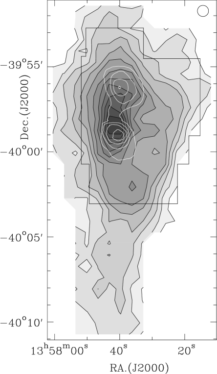
Figure 2: Map of integrated emission of ¹³C0 (1–0): $\int$$T_{A}^{*}$ dv from $-8$ $\mathrm{km\,s^{-1}}$ to $-4$ $\mathrm{km\,s^{-1}}$. The lowest contour and the contour increment is 1.2 $\mathrm{K\,km\,s^{-1}}$. The SEST half power beam size at the line frequency is shown in the upper corner. The extent of the $\mathrm{C^{18}O}$ mapping and the outline of the $\mathrm{C^{18}O}$  (2-1) emission is indicated in the overlay.

The bulk of the molecular material traced by C¹⁸O emission is distributed in a narrow North-South oriented lane with two prominent maxima. A less intense maximum is observed to the SW. Henceforth the three intensity maxima will be referred to as CG 12-N, CG 12-S and CG 12-SW. CG 12-S corresponds to the $\mathrm{C^{18}O}$  (2–1) maximum reported in White (1993).

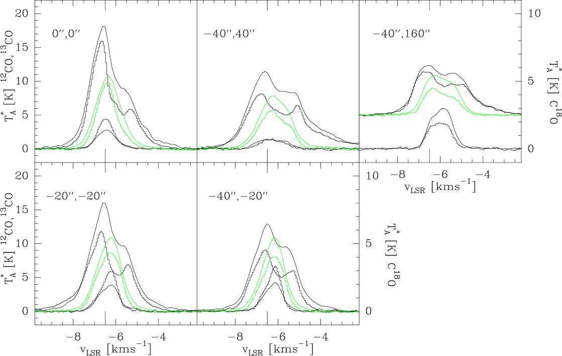
Figure 3: $\mathrm{{}^{12}CO}$ , $\mathrm{{}^{13}CO}$ and $\mathrm{C^{18}O}$ spectra observed towards five selected positions in CG 12. Offset from the map centre position is shown in arc seconds in the upper left corners of each panel. Line has been used for the (1–0) and histogram for the (2–1) transitions. The antenna temperature scale at left is for ¹²CO and ¹³CO spectra and the one on right for C¹⁸O. The velocity tick indicates velocity of $-$6.5 $\mathrm{km\,s^{-1}}$. The $\mathrm{{}^{12}CO}$ and $\mathrm{{}^{13}CO}$ spectra in position ($-$40″,160″) are offset from the zero level for clarity

The morphology of the cloud is similar in the two C¹⁸O transitions. However, there is a notable difference between the $\mathrm{C^{18}O}$ maxima. The observed C¹⁸O (1–0) emission is stronger than the C¹⁸O (2–1) emission in CG 12-N and CG 12-SW whereas in CG 12-S the opposite is the case. In CG 12-N the $\mathrm{C^{18}O}$ (1–0) line remains stronger than the (2–1) line even when expressed in the main beam brightness temperature scale.

Further details can be seen if Fig. 11 which reveals that the structure of the cloud is not as simple as Fig. 1 suggests. The most noticeable features are the following: CG 12-N is elongated in the North South direction at velocities $\leq-6.0$ $\mathrm{km\,s^{-1}}$ and in the East West direction at velocities $\geq-5.4$ $\mathrm{km\,s^{-1}}$. The position of the maximum $\mathrm{C^{18}O}$ (2–1) emission in CG 12-S moves from below the map centre position (marked with a cross in the Figure) at $-7.0$ $\mathrm{km\,s^{-1}}$ to a position 40″ west of this position at velocity $-5.9$ $\mathrm{km\,s^{-1}}$. An arc like feature connects CG 12-S and CG 12-SW at velocities from $-6.6$ $\mathrm{km\,s^{-1}}$ to $-6.2$ $\mathrm{km\,s^{-1}}$. The arc is less pronounced in the $\mathrm{C^{18}O}$ (2–1) transition.

The observed distribution of the $\mathrm{{}^{13}CO}$  (1–0) line emission towards CG12 is presented in Fig. 2. The extent of the $\mathrm{C^{18}O}$ mapping and the outline of the $\mathrm{C^{18}O}$  (2-1) emission is indicated in the overlay. The notable difference between the observed $\mathrm{C^{18}O}$ and $\mathrm{{}^{13}CO}$ emission is that there is only one $\mathrm{{}^{13}CO}$ maximum which is offset to NE from CG 12-S. In particular there is no indication of CG 12-N in the $\mathrm{{}^{13}CO}$ map.

¹²CO, ¹³CO and C¹⁸O (1–0) and (2–1) (pointed, long integration time) spectra in five selected positions in the cloud are shown in Fig. 3. The $\mathrm{{}^{12}CO}$ spectra observed at all positions in the figure are strongly self-absorbed. Therefore the $\mathrm{{}^{12}CO}$ line peak intensity, line half width and the line integral are not physically meaningful. Line wing emission due to a molecular outflow (White 1993) is seen in all $\mathrm{{}^{12}CO}$ spectra, also in the direction of CG 12-N which was not covered by the White (1993) observations.

3.2 High density tracers, mapping

In the optically thin case the critical density of the $\mathrm{C^{18}O}$ (1–0) transition is $\sim$650 $cm^{-3}$ and approximately ten times this value for the (2–1) transition (Rohlfs & Wilson (1999)). These $\mathrm{C^{18}O}$ lines are therefore excited already at low densities and their emission traces column density rather than number density. Therefore the $\mathrm{C^{18}O}$ intensity maxima were also mapped in the high density tracers (critical densities larger than $10^{5}cm^{-3}$) CS (2–1), $\mathrm{H^{13}CO^{+}(1-0)}$ and $\mathrm{DCO^{+}(2-1)}$ using 20″ spacing. A 4 by 4 point map with the same spacing was obtained in CG 12-S in the CS (3–2) line.

Contour maps of the CS (2–1), CS (3–2), H¹³CO⁺ and DCO⁺ line integral in CG 12 superposed on the $\mathrm{C^{18}O}$  (2–1) emission (grey scale) are shown in Fig. 4. CG 12-N was not mapped in CS (3–2). The CS (2–1) emission peaks at the position of the $\mathrm{C^{18}O}$ (2–1) the maximum in CG 12-S. In other molecules the maximum is shifted to SE from the $\mathrm{C^{18}O}$ maximum. As $\mathrm{DCO^{+}}$ traces high density gas the CG 12-S $\mathrm{DCO^{+}}$ maximum will be referred to as the $\mathrm{DCO^{+}}$ core.

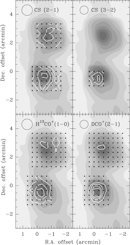
Figure 4: Contour maps of the observed CS (2–1), CS (3–2), $\mathrm{H^{13}CO^{+}(1-0)}$ and $\mathrm{DCO^{+}(2-1)}$ distributions in CG 12 superposed on a grey scale map of the $\mathrm{C^{18}O}$  (2–1) emission.   The positions observed in each molecule are indicated. The corresponding SEST beam size at the observed frequencies is indicated in the upper left corner of each panel. In the CS (2–1) and CS (3–2) maps the lowest contour value is 0.5 $\mathrm{K\,km\,s^{-1}}$ and the increments are 0.5 $\mathrm{K\,km\,s^{-1}}$ and 0.3 $\mathrm{K\,km\,s^{-1}}$, respectively. In the $\mathrm{H^{13}CO^{+}(1-0)}$ and $\mathrm{DCO^{+}(2-1)}$ maps the lowest contour value and its increment are 0.15 $\mathrm{K\,km\,s^{-1}}$. The maximum values of the CS (2–1), CS (3–2), $\mathrm{H^{13}CO^{+}(1-0)}$ and $\mathrm{DCO^{+}(2-1)}$ emission are 2.2 $\mathrm{K\,km\,s^{-1}}$, 1.3 $\mathrm{K\,km\,s^{-1}}$, 0.58 $\mathrm{K\,km\,s^{-1}}$ and 0.77 $\mathrm{K\,km\,s^{-1}}$, respectively. The offset from the map zero position is shown on the axes.

3.3 $\mathrm{C^{18}O}$ and high density tracers: pointed observations

Pointed, long integration time CS (2–1), (3–2), $\mathrm{C^{34}S}$(2–1), $\mathrm{H^{13}CO^{+}}$ (1–0), $\mathrm{DCO^{+}}$ (2–1) and $\mathrm{N_{2}H^{+}}$ (1–0) spectra in the same positions as in Fig 3 are shown in Fig. 5. The integration time of the CS (3–2) line at position ($-$40″,$-$20″) is only 2.5 minutes and is therefore noisier than the two other CS (3–2) lines. $\mathrm{N_{2}H^{+}}$ (1–0) line consists of seven hyperfine components and only the unblended $\mathrm{N_{2}H^{+}}$ (1–0) (F₁, F$=0,1\rightarrow 1,2$) component is shown in Fig. 5.

The $\mathrm{C^{34}S}$ line was observed in three positions. These spectra together with the CS (2–1) and (3–2) spectra observed at the same positions are shown in Fig. 6.

The $\mathrm{N_{2}H^{+}}$ spectra showing all the hyperfine components in the three observed positions are shown in Fig. 7. Also the hyperfine component fits (assuming optically thin emission and one velocity component) and their residuals are shown.

3.3.1 CG 12-S

Near the centre of the $\mathrm{DCO^{+}}$ core (position $-$20″,$-$20″) the $\mathrm{H^{13}CO^{+}}$, $\mathrm{DCO^{+}}$ and $\mathrm{N_{2}H^{+}}$ lines are nearly symmetric and centered at velocity $-6.5$ $\mathrm{km\,s^{-1}}$. The $\mathrm{C^{18}O}$ lines are skewed and the maximum intensity is redshifted from the $\mathrm{DCO^{+}(2-1)}$ peak velocity. Going to the West (position $-$40″, $-$20″) the redshifted side of the $\mathrm{C^{18}O}$ lines becomes more intense. Low intensity wing-like emission is observed in the $\mathrm{C^{18}O}$ and CS (2–1) lines in the direction of the $\mathrm{DCO^{+}}$ core and position (0″,0″).

The $\mathrm{N_{2}H^{+}}$ line in the position ($-$20″,$-$20″) can be fit with a single velocity component centred at $-$6.56 $\mathrm{km\,s^{-1}}$ (Fig. 7, lower panel). Due to the 0.73 $\mathrm{km\,s^{-1}}$ line half width the hyperfine components are blended and the hyperfine structure is only marginally resolved. The signal-to-noise ratio of the spectrum is not sufficient to make a meaningful fit of the line total optical depth, $\tau_{\rm tot}$. The estimated $\tau_{\rm tot}$ upper limit in this position is 5.

3.3.2 CG 12-N

In CG 12-N  (position $-$40″,160″) the $\mathrm{C^{18}O}$ lines are nearly symmetric but not gaussian. The emission from the high density tracers is weak when compared to that observed in CG 12-S.

The $\mathrm{C^{34}S}$ line was observed in two positions in CG 12-N (Fig. 6). The CS(2–1) and (3–2) line profiles in these positions are not gaussian and may be composed of two or three components. The peak intensity of the $\mathrm{C^{34}S}$ (2–1) line is redshifted with respect to the peak of the CS (3–2) line which itself is redshifted with respect to the CS (2–1) line. The latter line peaks approximately at the same velocity as the $\mathrm{C^{18}O}$ lines.

The observed ionic lines ($\mathrm{DCO^{+}}$ (2-1), $\mathrm{H^{13}CO^{+}}$ (1-0) and $\mathrm{N_{2}H^{+}}$ (1–0)) are offset +0.5 $\mathrm{km\,s^{-1}}$ in velocity with respect to the $\mathrm{C^{18}O}$ lines and peak at a velocity where especially the C¹⁸O (2–1) line intensity is low.

N₂H⁺ (1–0) was observed in the same two positions as $\mathrm{C^{34}S}$. Contrary to the CS lines, the observed $\mathrm{N_{2}H^{+}}$ lines are identical within the noise (Fig. 7, two upper panels). The SEST beam is the same at CS (2–1) and $\mathrm{N_{2}H^{+}}$ (1–0) frequencies. A hyperfine component fit to the CG 12-N $\mathrm{N_{2}H^{+}}$ lines gives a 0.65 $\mathrm{km\,s^{-1}}$ broad line at $-5.41$ $\mathrm{km\,s^{-1}}$. The estimated $\tau_{\rm tot}$ upper limit in position ($-$40″,$-$160″) is 2.

To rule out that the observed intensity/velocity structure described above is due to calibration, pointing or frequency setting problems, the observations were carefully checked by observing the C¹⁸O and the DCO⁺, H¹³CO⁺ and CS lines after each other and making pointing checks before and after observations. Also, e.g., the line pair DCO⁺ (2–1) and $\mathrm{C^{18}O}$ (1-0) could be observed simultaneously with a dual receiver, thus excluding relative pointing errors.

Figure 5: Spectra of $\mathrm{C^{18}O}$ and molecules sensitive to number density towards the same positions as shown in Fig. 3. Only the unblended hyperfine $\mathrm{N_{2}H^{+}}$  (1–0) (F₁, F$=1,0\rightarrow 1,2$) component is shown. The velocity tick indicates a velocity of $-$6.5 $\mathrm{km\,s^{-1}}$. $\mathrm{C^{18}O}$ (1–0), CS (2–1) and $\mathrm{H^{13}CO^{+}}$ lines are plotted using continuous line. The panel lower right is a blowout of the upper right panel showing only the lines tracing high number density.

Figure 6: CS (2–1), (3–2) and $\mathrm{C^{34}S}$ (1–0) spectra observed in the direction of CG 12-N (the two upper panels) and CG 12-S (the lower panel)

.

Figure 7: $\mathrm{N_{2}H^{+}}$  (1–0) spectra observed in the direction of CG 12-N (the two upper panels) and CG 12-S (the lower panel). The seven component hyperfine structure fit and the resulting residuals are shown

4 Comparison with observations at other wavelengths

The $\mathrm{C^{18}O}$  (2–1) contour map superposed on the blue SERC-J DSS image is shown in Fig. 8. The bright optical reflection nebula NGC 5367 lies in front of CG 12-S whereas CG 12-N is in the direction of an optically heavily obscured region which is clearly seen in the inset. A 1.2 mm source (Haikala 2006, in preparation) coincides with the position of the CG 12-N $\mathrm{C^{18}O}$ maximum.

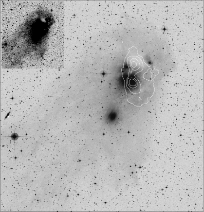
Figure 8: Contour map of the $\mathrm{C^{18}O}$  (2–1) emission superposed on the optical (DSS blue) image of NGC 5367. The image is also shown in the inset but using an intensity scale which better brings out the surface emission. The linear size of the image is 32′by 32′.

A Ks band image (Haikala 2006, in preparation) of CG 12 is shown in Fig. 9. Superposed on the image are the contours of the $\mathrm{{}^{12}CO}$ (2–1) molecular outflow line wing emission (White 1993). In the insets the $\mathrm{C^{18}O}$  (2–1) and $\mathrm{DCO^{+}}$ contour maps are superposed together with the positional uncertainty ellipses of IRAS point sources IRAS 13546-3941 and IRAS 13547-3944. IRAS 13547-3944 does not coincide with the binary h4636 (the base of the binary star emission is saturated due to the intensity scale which was chosen to emphasize the low intensity surface emission).

A cone like nebulosity with a bright head is seen projected on the $\mathrm{DCO^{+}}$ core in Fig. 9. The apex of the cone is located just off the tip of the red shifted and below the end of the blue shifted, collimated CO outflow lobes of White (1993). A compact 1.2 mm source (Haikala 2006, in preparation) coincides with the $\mathrm{DCO^{+}}$ core. The core does not have an associated point source but this could be due to the low spatial resolution of the IRAS satellite. A faint source would be masked by the strong nearby source IRAS 13547-3944. The NIR cone could be associated with the driving source of the outflow. The centre of the molecular outflow is offset from the position of IRAS 13547-3944 by $\sim$20″. It is unlikely that the point source is associated with the large outflow but it could be the driving force of the strong redshifted outflow lobe located $\sim$1′ NW of the point source nominal position.

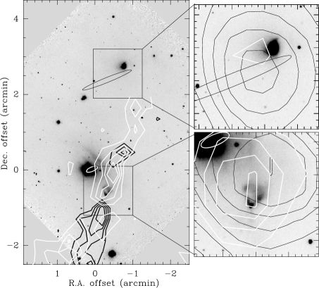
Figure 9: Ks–band image of CG-12 (Haikala 2006, in preparation). Contours of the blue (white contours) and redshifted (black) $\mathrm{{}^{12}CO}$  (2–1) line wing emission (White 1993) are also shown. The two insets show the CG 12-S and CG 12-N regions in detail. Superposed are the contours of $\mathrm{C^{18}O}$  (2–1) (black) and $\mathrm{DCO^{+}}$  (white) emission. The positional uncertainty ellipses of the IRAS point sources IRAS 13547-3944 in CG 12-S and IRAS 13546-3941 in CG 12-N are also shown.

Small areas of the size of the SEST HPBW at the $\mathrm{C^{18}O}$ (1–0) frequency in the centres of CG 12-N and CG 12-S have been mapped in the $\mathrm{C^{18}O}$ (3–2) (Haikala et al. 2006). The HPBW of the $\mathrm{C^{18}O}$ (3–2) observations is 19″ which is similar to the SEST HPBW of 24″  at the $\mathrm{C^{18}O}$ (2–1) frequency. In CG 12-S the $\mathrm{C^{18}O}$ (3–2) emission has a strong maximum in the same position as the maxima in the lower $\mathrm{C^{18}O}$ transitions. The line profile in position ($-$20″,$-$20″) agrees with the $\mathrm{C^{18}O}$ (2–1) line (Fig. 5). The $\mathrm{C^{18}O}$ (3–2) $T_{MB}$ peak line temperature in this position is, however, 10 K which is nearly twice the $\mathrm{C^{18}O}$ (2–1) $T_{MB}$ of 5.7 K. In CG 12-N (position ($-$40″,160″) the $\mathrm{C^{18}O}$ (3–2) line profile is similar to that of $\mathrm{C^{18}O}$ (1–0) but the $T_{MB}$ peak line temperature is 3 K which is lower than the corresponding values observed in $\mathrm{C^{18}O}$ (1–0) and (2–1) which are 4.3 K and 3.8 K, respectively.

5 $\mathrm{C^{18}O}$ fine scale structure

The half widths of the observed C¹⁸O lines in CG 12 cores range from 1.0 $\mathrm{km\,s^{-1}}$ (CG 12-S) to 1.3 $\mathrm{km\,s^{-1}}$ (CG 12-N). The $\mathrm{C^{18}O}$ channel-maps (Fig. 11) and observations of other molecules indicate, that the lines consist of more than one velocity component. The division of the cloud according to its appearance in the $\mathrm{C^{18}O}$ line integral maps (Fig. 1) into only three components, CG 12-N, CG 12-S and CG 12-SW, is therefore too coarse. The fine structure within the individual maxima is not seen because the lines are heavily blended in velocity.

5.1 Positive Matrix Factorization

Positive Matrix Factorization (PMF) has been used by Juvela et al. (1996) and Russeil at al. (2003) in the analysis of molecular line spectral maps. PMF assumes, that the ensemble of input spectra are composed of n individual line components (factors). Unlike the Principal Component Analysis PMF assumes that the individual components are positive. This makes the interpretation of the results more straightforward than in Principal Component Analysis where the results may contain negative components. No other assumptions are made of the shape of the factors. Each input spectrum can be reconstructed from the n PMF output factors by multiplying each factor by the weight assigned to it by PMF at the position and adding up the multiplied factors. A comparison of the results obtained with PMF analysis with those obtained using the analysis of channel maps and by the use of Principal component analysis is given Russeil at al. (2003).

PMF has been applied separately to the north and south parts of CG 12 but there is a small positional overlap between the two areas used in the analysis. The same dataset, which is shown in Fig. 11 was used in the analysis, i.e, the $\mathrm{C^{18}O}$  (2–1) data is binned to the same channel width as the $\mathrm{C^{18}O}$  (1–0) data. The PMF analysis is presented in Appendix A.

6 Discussion

6.1 $\mathrm{C^{18}O}$ as a tracer of molecular material

C¹⁸O emission is generally considered a good tracer of large scale structure of dark clouds and globules. However, $\mathrm{C^{18}O}$ photodissociation in the cloud envelopes and molecular depletion in the dense and cold cloud cores may restrict the number density interval where $\mathrm{C^{18}O}$ emission can be used as a direct measure of $\rm H_{2}$ column density (especially if the LTE approximation is used). Unlike $\mathrm{{}^{12}CO}$, the $\mathrm{C^{18}O}$ molecules are not shielded against photodissociation by strong $\rm H_{2}$ lines and further, the $\mathrm{C^{18}O}$ self-shielding is weaker than that of $\mathrm{{}^{12}CO}$. For $\mathrm{C^{18}O}$ the self-shielding is most efficient for the two lowest rotational levels with the largest populations. According to Warin et al. (1996), the consequence is that the J=1–0 transition becomes thermalized, whereas the higher transitions remain subthermally excited in the cloud envelopes. In the other extreme (pre-stellar cloud cores and protostellar envelopes) the CO molecule may vanish from gas phase because of depletion onto dust grains. Further complications in interpreting $\mathrm{C^{18}O}$ data are the possible strong gradients in the CO excitation temperature on the line of sight due to heating of the gas by newly born stars and protostellar objects. Time and temperature dependent chemistry like, e.g., deuterium fractionation, also complicates the comparison of $\mathrm{C^{18}O}$ data with that of other molecular species.

Depletion of molecules on dust grains takes place in the dense, quiescent and cold molecular cloud cores. CO and CS are among the first molecules to disappear from the gas phase but nitrogen bearing species like, e.g., $\mathrm{N_{2}H^{+}}$ and ammonia, seem to be able to resist depletion (Tafalla et al. (2002)). The $\mathrm{N_{2}H^{+}}$ and $\mathrm{DCO^{+}}$ lines in CG 12-N peak at a velocity of 5.4 $\mathrm{km\,s^{-1}}$  where the $\mathrm{C^{18}O}$ line emission is weak (Sect. 3.3). It is likely, that strong CO depletion has taken place in the gas traced by these two molecules in CG 12-N .

In CG 12-S the $\mathrm{C^{18}O}$ maximum is spatially offset from the $\mathrm{DCO^{+}}$ core. Deuterium fractionation reactions are favored in cold gas (e.g., Herbst (1982)) and therefore the relative abundance of $\mathrm{DCO^{+}}$ is enhanced in cold cloud cores. The relatively strong $\mathrm{DCO^{+}}$ emission observed in CG 12-S, the $\mathrm{DCO^{+}}$ core, could indicate that fractionation has indeed taken place. If the molecules in CG 12-S were heavily depleted in the cold $\mathrm{DCO^{+}}$ core one would not expect CS (3–2) or $\mathrm{H^{13}CO^{+}}$ to outline the core like they do (also $\mathrm{DCO^{+}}$ will be finally depleted).

The observed $\mathrm{{}^{12}CO}$ (1–0) and (2–1) line temperatures in CG 12-S (Fig. 3) are high. The lines are self reversed so the actual line peak temperatures must be even higher. This indicates that the CO excitation temperature is in excess of 30 K in the part of the cloud which is traced by the observed $\mathrm{{}^{12}CO}$ emission. White (1993) suggests that either h4636 or IRAS 13547-3944 is the heating source. The $\mathrm{{}^{12}CO}$ and $\mathrm{{}^{13}CO}$ optical depth is high and unlike $\mathrm{C^{18}O}$ these CO isotopoloques are likely to trace only the surface of the molecular cloud associated with CG 12. The observed $\mathrm{C^{18}O}$ (3–2) $T_{MB}$  peak temperature of 11 K in CG 12-S also points at a high $\mathrm{C^{18}O}$ excitation temperature (Haikala et al. 2006). However, the observed relative $\mathrm{C^{18}O}$ (2–1) and (1–0) line intensities in CG 12-S are not compatible with $\mathrm{C^{18}O}$ $T_{ex}$ values higher than 20 K.

6.2 PMF: The interpretation

One should be cautious in interpreting the PMF results. Even though the fit to the $\mathrm{C^{18}O}$ (1–0) and (2–1) data is good, all the PMF factors do not necessarily describe real cloud components. The structure of the cloud can, however, be discussed with some confidence when the PMF fit results are considered with the information provided by other available molecular line, mm continuum and NIR-FIR data.

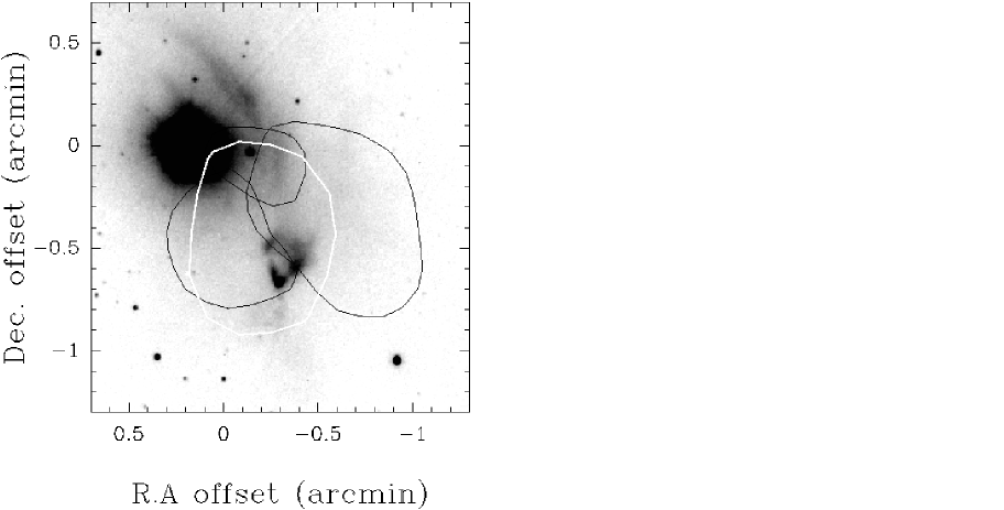
Figure 10: The CG 12-S $\mathrm{C^{18}O}$ (2–1) 1s, 2s and 3s (from East to West) factor peak emission positions (0.8 K $\mathrm{km\,s^{-1}}$ contours) and $\mathrm{DCO^{+}}$ core position  (white) superposed on the SOFI Ks band image. Offsets from the map zero position are shown in arcminutes. The SEST beam at the $\mathrm{C^{18}O}$  (2–1) frequency is 0.37 arcminutes

6.2.1 CG 12-S

The location of the CG 12-S $\mathrm{C^{18}O}$ (2–1) PMF factor maxima relative to the NIR cone (and the mm continuum source) in the centre of the $\mathrm{DCO^{+}}$ core is shown in Fig. 10. From East to West the factors are 1s, 2s and 3s. The centres of the maxima differ in position by about one SEST beam size at 220 GHz, 24″.

The data would seem to implicate that CG 12-S is fragmented into three individual cores. If this were the case one would expect that the 2s factor would coincide with the $\mathrm{DCO^{+}}$ core because the 2s centre of line velocity is the same as that of $\mathrm{DCO^{+}}$. Even though the 3s factor is the strongest in CG 12-S it is detected only as an asymmetry in the $\mathrm{DCO^{+}}$ and CS lines in Figs. 5 and 6. CO is ubiquitous and easily excited and therefore it can be detected at much lower densities than the high density tracers, $\mathrm{DCO^{+}}$ and CS (3–2), which trace the $\mathrm{DCO^{+}}$ core. The bulk of the observed $\mathrm{C^{18}O}$ emission may have its origin in the part of the cloud where the density is lower and the excitation temperature higher than in the $\mathrm{DCO^{+}}$ core.

This leads to a model where most of the observed $\mathrm{C^{18}O}$ emission traces rather the surface of the dense and cold cloud core (the $\mathrm{DCO^{+}}$ core) or a separate, adjacent cloud component, than the core itself. The observed CS (2–1) distribution, which is similar to $\mathrm{C^{18}O}$ in CG 12-S (Fig. 4), is in accord with this model. Much of the observed CS (2–1) emission is known to originate in cloud envelopes and not in the dense cores. The CS (3–2) effective critical density is higher than that of CS (2–1) and therefore it traces the dense gas deeper in the cloud than CS (2–1).

The possible interaction of the collimated molecular outflow detected by White (1993) with the cloud core further complicates the interpretation of the molecular line data. The centre of the outflow is located in the direction of the $\mathrm{DCO^{+}}$ core and it is not unlikely that the outflow can produce weak $\mathrm{C^{18}O}$ line wings and that it can raise the CO excitation temperature locally. Weak line wings are also observed in the CS (2–1) line in Fig. 5. It is argued that the weak $\mathrm{C^{18}O}$ red and blue shifted line wing emission near the $\mathrm{DCO^{+}}$ core is produced by the interaction of the collimated molecular outflow with the parent cloud. The line wings would be described by the PMF factors 1s and 4s. For the latter factor this would consists only of the emission immediately to the west of the $\mathrm{DCO^{+}}$ core.

The CG 12-S $\mathrm{C^{18}O}$ (3–2) map in Haikala et al. (2006) covers only the very centre of CG 12-S. The $\mathrm{C^{18}O}$ (3–2) line peak velocity and the intensity distribution is in accordance with the elongated shape of the 3s component in Fig. 10. The maximum of the 3s factor is compact and lies on the outflow axis only $\sim$20″ away from the apex of the NIR cone (Fig. 9), the putative position of the outflow driving source. This suggest, that the high 3s $\mathrm{C^{18}O}$ line intensities and the molecular outflow could be connected.

6.2.2 CG 12-N

PMF produces a seemingly straightforward solution for CG 12-N. However, the available data from molecules other than $\mathrm{C^{18}O}$ and the 1.2 mm continuum emission deny such a simple solution. As argued in Sect. 6.1 it is likely that the cloud component traced by $\mathrm{DCO^{+}}$ and $\mathrm{N_{2}H^{+}}$ is heavily depleted. If this is the case $\mathrm{C^{18}O}$ only probes the undepleted part of CG 12-N.

6.3 Cloud physical properties

A straightforward division of the CG 12 molecular cloud into three homogeneous components, CG 12-N, CG 12-S and CG 12-SW, is not possible. The good velocity resolution and the high signal to noise ratio of the data allows one to divide the $\mathrm{C^{18}O}$ data into separate components. However, the derivation of the cloud or core physical properties calls for a detailed three dimensional non-LTE model which takes into account both the molecular depletion, the varying density and excitation conditions. Such a model is beyond the scope of this paper and will be left for the future. The LTE-approximation approach is used instead of a sophisticated model to make a zeroth order estimate of the masses of the three $\mathrm{C^{18}O}$ maxima, CG 12-N, CG 12-S and CG 12-SW. An average $\mathrm{C^{18}O}$ excitation temperature for each maximum is estimated using the observed relative $\mathrm{C^{18}O}$ (2–1) and (1–0) line intensities.

6.3.1 Mass and column density estimation

The observed $T_{A}^{*}$ line temperatures were converted into main beam temperatures using the beam efficiencies in Table LABEL:figure:table1. The $\mathrm{C^{18}O}$ excitation temperatures were estimated from the $\mathrm{C^{18}O}$ (1–0) and (2–1) data assuming optically thin $\mathrm{C^{18}O}$ emission and LTE. This assumes that the observed emission in both transitions originates in the same volume of gas at a constant excitation temperature. The observed $\mathrm{C^{18}O}$ line $T_{MB}$(2–1)/ $T_{MB}$(1–0) ratio is 1.8 in CG 12-S, compatible with an excitation temperature near 15 K. In CG 12-N and CG 12-SW this ratio is one or less indicating excitation temperatures of the order of 10 K.

The masses of CG 12-N, CG 12-S and CG 12-SW are calculated without dividing them into smaller components. The spectra between declination offsets (including the limits) $-$120″ and +60″ were assigned to CG 12-S. The spectra above and below these limits were assigned to CG 12-N and CG 12-SW, respectively. An average $\mathrm{C^{18}O}$ excitation temperature of 10 K is now assumed for CG 12-N and CG 12-SW and 15 K for CG 12-S. The adopted $\mathrm{C^{18}O}$ abundance is 2.0 $10^{-7}$. This results in calculated total masses of   34, 96, and 110 $\mathrm{M}_{\odot}$ for CG 12-SW, CG 12-S and CG 12-N, respectively, when $\mathrm{C^{18}O}$ (1–0) data is used. If $\mathrm{C^{18}O}$ (2–1) data is used the masses are 14, 49 and 53 $\mathrm{M}_{\odot}$. The maximum $T_{MB}$  line integrals can be used to estimate the $\rm H_{2}$ column densities in the corresponding beams. The calculated maximum column densities in the $\mathrm{C^{18}O}$ (1–0) beam are 1.3 $10^{22}$, 1.8 $10^{22}$ and 2.7 $10^{22}$ $cm^{-2}$ for CG 12-SW, CG 12-S and CG 12-N, respectively. For the $\mathrm{C^{18}O}$ (2–1) beam the corresponding values are 6.4 $10^{21}$, 1.6 $10^{22}$ and 1.8 $10^{22}$ $cm^{-2}$.

The masses calculated from the $\mathrm{C^{18}O}$ (1–0) data are approximately twice higher than from the (2–1) data. The LTE approximation assumes that all the $\mathrm{C^{18}O}$ rotational states are thermalized. However, according to Warin et al. (1996) only the lowest $\mathrm{C^{18}O}$ rotational state is thermalized in dark clouds and the higher states are subthermally excited. The subthermal excitation would be stronger in the relatively low density cloud envelope than in the more dense core. The subthermal level population leads to an underestimation of the cloud mass when calculated from the $\mathrm{C^{18}O}$ (2–1) data. This could be a partial explanation for the large discrepancy between the masses calculated using $\mathrm{C^{18}O}$ (1–0) and (2–1) data.

Strong $\mathrm{C^{18}O}$ (3–2) emission (maximum $T_{MB}$ $\sim$11 K) distributed similar to the 3s PMF factor was detected by Haikala et al. (2006) in the centre of CG 12-S . The $\mathrm{C^{18}O}$ (3–2) data was modelled with a compact (60″ to 80″ diameter) and hot (80 K $\lesssim$$T_{ex}$$\lesssim$ 200 K) optically thin clump of $\sim$ 1.6 $\mathrm{M}_{\odot}$. The high temperature was derived from the $T_{MB}$ ($\mathrm{C^{18}O}$ (3–2))/$T_{MB}$ ($\mathrm{C^{18}O}$ (2–1)) ratio. However, $T_{MB}$ ($\mathrm{C^{18}O}$ (2–1))/$T_{MB}$ ($\mathrm{C^{18}O}$ (1–0)) ratio for the CG 12-S PMF factor 3s is not compatible with such a high temperature. This could be due to, e.g., contribution from a subthermally excited cool cloud envelope to the $\mathrm{C^{18}O}$ (1–0) emission. The LTE mass calculated from the $\mathrm{C^{18}O}$ (2–1) 3s component within the area modelled in Haikala et al. (2006) is 4.1 $\mathrm{M}_{\odot}$ when a $T_{ex}$ of 15 K is assumed. The discrepancy in the calculated excitation temperatures and masses highlights the uncertainties when LTE approximation is used and only data of the two lowest $\mathrm{C^{18}O}$ transitions are available. In contrast to CG 12-S the $\mathrm{C^{18}O}$ $T_{ex}$ and the LTE mass of CG 12-N correspond well to the modelled values using the the three transitions (Haikala et al 2006).

6.4 Summary

The analysis of the spectral lines presented above deliver a complicated picture of CG 12. Even though the spectral lines are relatively narrow the analysis reveals a rich structure in line shape and velocity. Probable depletion of molecules on dust grains in CG 12-N further complicates the interpretation. The cloud parameters derived using the LTE analysis are highly uncertain. However, if the molecular line observations are combined with the available optical, NIR, FIR and mm continuum data the cloud structure can be discussed with some confidence.

6.4.1 CG 12-N

CG 12-N harbors a compact, cold mm source and the detected relatively weak molecular emission in high density tracers is probably associated with this source. Much of the molecular material associated with this cloud component is likely to be highly depleted onto dust. The observed strong $\mathrm{C^{18}O}$ emission towards CG 12-N originates therefore in the envelope of this depleted core or in a separate entity seen in the same line of sight. $\mathrm{{}^{12}CO}$ observed in the direction of CG 12-N has line wing emission indicating molecular outflow. It is not known if this outflow is connected to the outflow in CG 12-S or if it is local and originates in CG 12-N .

6.4.2 CG 12-S

The bulk of the observed $\mathrm{C^{18}O}$ emission does not trace the gas associated with the compact cloud core detected in $\mathrm{H^{13}CO^{+}}$, $\mathrm{DCO^{+}}$ and CS (3–2) lines. Most likely the $\mathrm{C^{18}O}$ emission traces only the surface of this core. The moderate $\mathrm{C^{18}O}$ line wing emission, probably due to interaction of the highly collimated molecular outflow with the surrounding gas, further complicates the interpretation.

The molecular line data presented in this paper combined with the molecular outflow data from White (1993), the NIR imaging and mm dust continuum data (Haikala 2006, in preparation) shows that the outflow centre coincides with the mm continuum source and the NIR cone in the centre of the $\mathrm{DCO^{+}}$ core. The strong point source IRAS 13547–3944 is offset from the mm source and from h4636. This point source could, however, be the driving source for the strong redshifted outflow lobe north of CG 12-S.

6.4.3 CG 12-SW

CG12-SW is inconspicuous when compared to the two stronger $\mathrm{C^{18}O}$ maxima. No signs of star formation have been found in its direction and it is therefore either still in pre-star formation phase or its density-temperature structure is such that no star formation will take place. The arc like feature which connects CG 12-S and CG 12-SW at velocities from $-6.6$ $\mathrm{km\,s^{-1}}$ to $-6.2$ $\mathrm{km\,s^{-1}}$ in Fig. 11 suggests that CG 12-SW might be connected with CG 12-S.

7 Conclusions

We have performed a detailed, high signal-to-noise ratio, mm line study of CG 12 in various molecular transitions, principally of C¹⁸O (1–0) and C¹⁸O (2–1), as well as in molecular lines probing dense material, and have obtained the following results:

1. The C¹⁸O line emission is distributed in a 10$\arcmin$ North-South elongated lane with two strong, compact maxima, CG 12-N and CG 12-S, and a weaker maximum, CG 12-SW.

2. High density tracers CS (2–1), (3-2), $\mathrm{DCO^{+}}$ and $\mathrm{H^{13}CO^{+}}$ are detected in both strong $\mathrm{C^{18}O}$ maxima. Emission from these molecules is weak in CG 12-N but in CG 12-S it defines a compact core (referred to as $\mathrm{DCO^{+}}$ core) which is spatially offset from the $\mathrm{C^{18}O}$ maximum.

3. The emission from the high density tracers in CG 12-N takes place at a velocity where emission from $\mathrm{C^{18}O}$ is weak. The molecules associated with the cloud component detected in high density tracers are likely to be heavily depleted.

4. Positive Matrix Factorization was applied to study the cloud $\mathrm{C^{18}O}$ fine scale structure. The observed strong $\mathrm{C^{18}O}$ emission in CG 12-N (PMF factor 2n) originates in the envelope of the depleted cloud component or in a separate entity seen in the same line of sight. In CG 12-S the most intense PMF factor 3s traces warm gas on the surface of the $\mathrm{DCO^{+}}$ core or a separate adjacent cloud component.

5. The driving source of the collimated molecular outflow detected by White (1993) lies in the $\mathrm{DCO^{+}}$ core.

6. The average $\mathrm{C^{18}O}$ LTE mass is $\sim$80 M_☉ for CG 12-N, $\sim$70 M_☉ for CG 12-S and $\sim$20 M_☉ for CG 12-SW. These numbers can only be considered as a zeroth order estimate because of the uncertainty in defining the $\mathrm{C^{18}O}$ excitation temperature and possible molecular depletion in the $\mathrm{C^{18}O}$ maxima.

7. If the distance to CG 12, 630 pc, is correct the linear size and the mass of this cometary globule approaches that of a typical low mass star forming region like eg. Chamaeleon I.

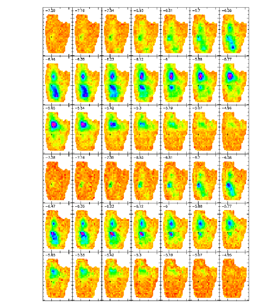
Figure 11: $T_{A}^{*}$ channel map of the C¹⁸O (1–0) emission (upper three rows) and C¹⁸O (2–1) (lower three rows). The colour scale is the same for both transitions. The LSR velocity is indicated in the upper left corners of the panels. Each pixel corresponds to a single observed position but the C¹⁸O (2–1) data is binned in this figure to the same channel width as the (1–0) transition, 0.116 $\mathrm{km\,s^{-1}}$. The highest intensity in the panels is $\sim 3.0$ K. The cross in the panels is located in the map centre position.

Appendix A Positive Matrix Factorization analysis of CG 12

A.1 CG 12-N

The results of the PMF, assuming three factors, to observed $\mathrm{C^{18}O}$  (1–0) and (2–1) data in CG 12-N are shown in Figs. 12 and 13. The uppermost panels show the three fitted PMF factors. The area under each factor is normalized to one. The histogram superposed on the rightmost factor in Fig 13 indicates the velocity resolution of the input data. The intensity distribution of the PMF factors in CG 12-N are shown in the lower three panels.

The PMF reproduces well the velocity structure displayed in Fig. 11. The fits to the $\mathrm{C^{18}O}$  (1–0) and (2–1) data are independent of each other. Therefore it is encouraging that the PMF output factors for both $\mathrm{C^{18}O}$ transitions are similar in velocity and in spatial distribution. Because of the unambiguity of the fits for both transitions the factors, centered at $-6.6$, $-5.9$ and $-5.4$ $\mathrm{km\,s^{-1}}$, are referred to in the following as 1n, 2n and 3n, respectively.

Figure 12: Upper panel: the basic spectral profiles (factors) calculated by the PMF in CG 12-N  (three factor fit), $\mathrm{C^{18}O}$ (1–0) data. Lower panels: maps of the weights of the basic factors. The lowest contour level and increment are 0.2 $\mathrm{K\,km\,s^{-1}}$. Offsets from the centre position of the original $\mathrm{C^{18}O}$ map are shown in arcminutes on the x and y axes.

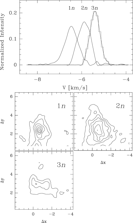
Figure 13: As Fig. 12 but for $\mathrm{C^{18}O}$ (2–1) data. Factor 3n in the upper panel has been plotted also as a histogram to indicate velocity resolution of the input/output spectra.

The PMF factors, 1n, 2n and 3n, are distributed in a north-south oriented ridge, in a pear shaped body and a narrow east-west ridge, respectively. The 3n factor lies at the velocity where the emission from the $\mathrm{H^{13}CO^{+}}$, $\mathrm{DCO^{+}}$, and $\mathrm{N_{2}H^{+}}$ is at maximum. Even though this factor is not readily evident in the individual spectra PMF finds it in both $\mathrm{C^{18}O}$ transitions. Factors 2n and 3n are symmetric but factor 1n has blue and redshifted wing like emission, especially in the (1–0) transition. According to the PMF fit the high $T_{A}^{*}$ (C¹⁸O (1–0))/$T_{A}^{*}$ (C¹⁸O (2–1)) ratio observed in the direction of CG 12-N is due to the factor 2n.

If the number of factors in the PMF is chosen to be four PMF divides in essence the factor 1n into two, leaving the two other factors untouched. The spatial distribution of the split up factors is similar to that of the 1n in the three-factor PMF. If the number of factors is further increased to five the result is similar to that with four factors plus a fifth factor which has nearly zero intensity, ’empty’ field, in the map. The three factors are therefore sufficient to produce the velocity structure evident in Fig. 11 and increasing the number of factors does not improve the fit significantly.

A.2 CG 12-S and CG 12-SW

The results of the PMF fits, assuming four factors, to both observed $\mathrm{C^{18}O}$ transitions in CG 12-S are shown in Figs. 14 and 15. The location of the $\mathrm{DCO^{+}}$ core is shown with a dashed contour in the figures. The factors, centered at $-6.8$, $-6.4$, $-6.2$ and $-5.8$ $\mathrm{km\,s^{-1}}$, will be referred to as 1s to 4s, respectively.

The most redshifted factor 4s covers the very northern part of the region and is close in velocity to the 2n factor in CG 12-N. It is natural to consider that this factor is due to emission extending from CG 12-N to CG 12-S. Also the very faint emission observed in the northern part of the field in other three factors is at least partly due to emission from CG 12-N.

The emission from the most blueshifted factor 1s is concentrated just below the (0,0) position. The 2s factor represents the arc seen in Fig. 11 which connects CG 12-S and CG 12-SW . There is a small size local maximum in the $\mathrm{C^{18}O}$  (2–1) 2s factor north of the $\mathrm{DCO^{+}}$ core. Even though this local maximum is not seen in the $\mathrm{C^{18}O}$  (1–0) 2s factor, there is extended emission at its location. The southern part of the arc is more intense in the (1–0) transition than in the (2–1). The maximum of the southern extension coincides with CG 12-SW. The emission from the 3s factor peaks west of the $\mathrm{DCO^{+}}$ core and is seen in both transitions.

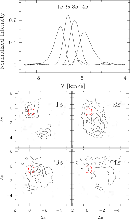
Figure 14: Upper panel: the basic spectral profiles calculated by the PMF in CG 12-S  (four factor fit), $\mathrm{C^{18}O}$ (1–0) data. Lower panels: the maps of the intensity of the basic factors. The factor numbers correspond to the numbers in the upper panel. The lowest contour level and increment is 0.2 $\mathrm{K\,km\,s^{-1}}$. The dashed contour outlines the $\mathrm{DCO^{+}}$ core.

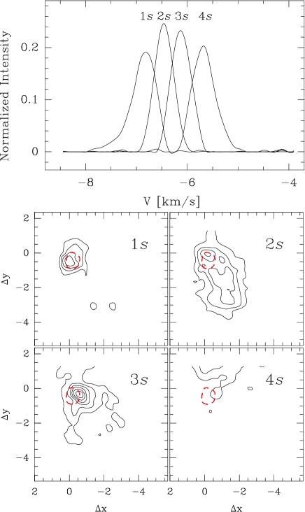
Figure 15: As Fig. 14 but for $\mathrm{C^{18}O}$ (2–1) data.

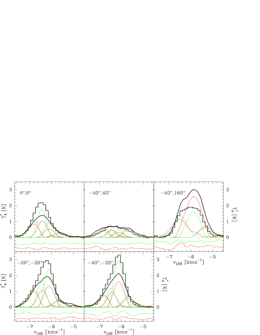
Figure 16: The PMF fit to the $\mathrm{C^{18}O}$ lines in the selected positions positions in Fig. 5. The observed $\mathrm{C^{18}O}$ (2–1) and (1–0) lines are plotted with a heavy histogram and line, respectively. The green and red lines show the fitted PMF $\mathrm{C^{18}O}$ (2–1) and (1–0) factors, respectively. The residuals of the fits are shown in the lower part of each panel.

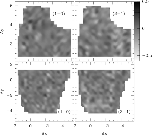
Figure 17: The PMF fit residuals in the $\mathrm{K\,km\,s^{-1}}$scale.

A.3 Individual line profiles

The PMF fits to the $\mathrm{C^{18}O}$ lines in the same selected positions as in Fig. 5 are shown in Fig. 16. The residuals obtained by subtracting the added up PMF factors from the observed lines are shown below the lines in the figure. A grey scale map of all the PMF fit residuals is shown in Fig. 17. One should stress that, unlike a gaussian multicomponent fit to a single spectrum, PMF fits, in this case 3 (CG 12-N) or 4 (CG 12-S) factors into all the input spectra simultaneously. Neither the shape nor the velocity of the factors is fixed in the fit. The two $\mathrm{C^{18}O}$ transitions were fit separately and PMF could have used factors differing in profile and velocity for the two transitions. The fitted PMF factors are, however, similar both in shape and velocity. The residuals shown in Figs. 16 and 17 are small and demonstrate that PMF produces a good fit to the data.

The largest residual in Fig. 16 takes place in the blue shifted side of the $\mathrm{C^{18}O}$  (1–0) line in the centre of CG 12-N  (position $-$40″,160″). This would imply that the blue shifted wing of factor $\mathrm{C^{18}O}$ (1–0) 1n is too strong. A closer comparison of the input data and PMF results reveals that similar deviations take place for three other $\mathrm{C^{18}O}$  (1–0) spectra around the position above. The $\mathrm{C^{18}O}$  (1–0) line profiles farther away from the CG 12-N centre actually do have a more prominent blue shifted wing than the four above mentioned spectra. The large number of spectra with good fits outweighs the less optimal fit for the spectra in the centre of CG 12-N. The residuals shown in Fig. 16 for the remaining four spectra in CG 12-S are smaller than in position ($-$40″,160″).