Optical properties and spatial distribution
of MgII absorbers from SDSS image stacking

Abstract

We present a statistical analysis of the photometric properties and spatial distribution of more than 2,800 MgII absorbers with $0.37<z<1$ and rest equivalent width $W_{0}(\lambda 2796)>0.8$Å detected in SDSS quasar spectra. Using an improved image stacking technique, we measure the cross-correlation between MgII gas and light (in the $g$, $r$, $i$ and $z$-bands) from 10 to 200 kpc and infer the light-weighted impact parameter distribution of MgII absorbers. Such a quantity is well described by a power-law with an index that strongly depends on absorption rest equivalent width $W_{0}$, ranging from $\sim-1$ for $W_{0}\lesssim 1$Å  to $\sim-2$ for $W_{0}\gtrsim 1.5$Å.

At redshift $0.37<z_{abs}\leq 0.55$, we find the average luminosity enclosed within 100 kpc around MgII absorbers to be $M_{g}=-20.65\pm 0.11$ mag, which is $\sim 0.5~{}L_{g}^{\star}$. The global luminosity-weighted colors are typical of present-day intermediate type galaxies. We then investigate these colors as a function of MgII rest equivalent width and find that they follow the track between spiral and elliptical galaxies in color space: while the light of weaker absorbers originates mostly from red passive galaxies, stronger systems display the colors of blue star-forming galaxies. Based on these observations, we argue that the origin of strong MgII absorber systems might be better explained by models of metal-enriched gas outflows from star-forming/bursting galaxies.

Our analysis does not show any redshift dependence for both impact parameter and rest-frame colors up to $z=1$. However, we do observe a brightening of the absorbers related light at high redshift ($\sim 50\%$ from $z_{abs}\sim 0.4$ to 1). We argue that MgII absorbers are a phenomenon typical of a given evolutionary phase that more massive galaxies experience earlier than less massive ones, in a downsizing fashion.

This analysis provides us with robust and quantitative constraints of interest for further modeling of the gas distribution around galaxies. As a side product we also show that the stacking technique allows us to detect the light of quasar hosts and their environment.

1. Introduction

Quasar absorption lines provide us with a unique tool to probe the gas content in the Universe with a sensitivity that does not depend on redshift. In order to use this information for investigating galaxy formation and evolution, characterizing the underlying population of galaxies seen in absorption is an important task to achieve.

In 1969, Bahcall & Spitzer suggested that metal absorption lines seen in quasar spectra are induced by large halos of gas around galaxies extending up to a hundred kpc. Since then, the study of quasar absorption lines has become an active field of investigation, but fundamental questions regarding the nature of this gas and its distribution around galaxies still remain.

Studies of absorber-galaxy connections began with the investigation of MgII systems. Such a choice results from a practical constraint: among the dominant ions in HI gas, MgII has the longest-wavelength resonance transition at the doublet $\lambda\lambda 2796.35,2803.53$. Several studies showed that MgII arises in gas spanning more than five decades of neutral hydrogen column density (Bergeron & Stasinska, 1986; Steidel & Sargent, 1992; Churchill et al., 2000), and at a similar time the first galaxies responsible for some metal absorption features were identified (Bergeron, 1986; Bergeron et al., 1987; Cristiani, 1987; Bergeron & Boissé, 1991). Steidel et al. (1994) then built a sample of 58 identified MgII systems and found that various types of galaxies with $\sim L^{\star}$ luminosities exhibit MgII absorption up to a radius of $R\sim 50h^{-1}$ kpc. For a review of results regarding the connection between MgII absorbers and galaxies see Churchill et al. (2005a). It is also interesting to mention that Bowen et al. (2006) recently reported the detection of MgII absorption around quasars.

While the connection between galaxies and metal absorbers has been clearly established, the origin of the absorbing gas and its properties remains unclear. Whether these absorption lines trace gas being accreted by a galaxy or outflowing from it is still a matter of debate. Recently the SDSS database has provided us with significantly larger samples of absorbers (by two orders of magnitude), allowing us to accurately measure a number of statistical properties such as the redshift distribution, $dN/dz$, and the distribution of absorber rest equivalent widths, $dN/dW_{0}$, which is now measured over more than a decade in $W_{0}$ (Nestor et al., 2005; Prochter et al., 2006). Unfortunately, physical models or numerical simulations reproducing these observations are still lacking. While efforts on the theoretical side are needed, additional statistical observational constraints are required, especially to characterize the spatial distribution of the gas around galaxies and their corresponding optical properties.

Previous attempts to constrain such properties of MgII absorbers have relied on deep imaging and spectroscopic follow-up of (arbitrarily faint) galaxies in the quasar field in order to identify a potential galaxy responsible for the absorption seen in the quasar spectrum. Such expensive studies have been limited to samples of a few tens of quasars. Moreover recent results have shown discrepancies in the inferred distributions of absorber impact parameters. Whereas Steidel et al. (1994) claimed that $\sim L^{\star}$ galaxies are surrounded by MgII halos extending up to $R\sim 50h^{-1}$ kpc, Churchill et al. (2005a) recently showed that a more systematic analysis reveals the same type of absorption up to $R\sim 100h^{-1}$ kpc in a number of cases. The different results apparently arise from different ways of preselecting the candidate galaxies for the spectroscopic follow-up. Furthermore, it is interesting to note that the recent detections of MgII around quasars (Bowen et al., 2006) reach similar distances. Estimating the distribution of absorber impact parameters without the use of any assumption is therefore needed.

It should be emphasized that the identification of a galaxy responsible for a given absorption feature is in general not a well defined process. Indeed it is always possible that an object fainter than the limiting magnitude, such as a dwarf galaxy, gives rise to the absorbing gas, or that more than one galaxy has a redshift consistent with that of the absorber system which is likely to happen in group environments. A well-defined quantity that can be obtained from observations and modeled theoretically is the cross-correlation between absorbers and the measured light within a given radius: $\langle W_{0}\,L\rangle(\theta)$.

In Zibetti et al. (2005a) we proposed a new approach to measure the systematic photometric properties of large samples of absorbing systems, which combines statistical analysis of both spectroscopic and imaging datasets of the Sloan Digital Sky Survey (hereafter SDSS York et al., 2000). As MgII lines can only be detected in SDSS spectra at $z\gtrsim 0.4$, the absorbing galaxies are only marginally detected in individual SDSS images at the lowest redshifts, and below the noise level otherwise. However, they do produce systematic light excesses around the background QSOs. Such excesses can be detected with a statistical analysis consisting of stacking a large number of absorbed QSO images. After having demonstrated the feasibility of this technique with EDR data (Zibetti et al., 2005a), we now extend our analysis to the SDSS DR4 sample, i.e., a dataset about twenty times larger.

Stacking analysis has the intrinsic limitation of only probing the mean or median value of a quantity for which the underlying distribution is not necessarily known. However, it can lead to detections of low-level signals not detectable otherwise. Moreover, one can also investigate the dependence of an observed quantity $O$ as a function of a set of parameters that describe a given sample. Some properties of the underlying distribution giving rise to $<O>$ can therefore be inferred.

Stacking approaches have provided us with valuable results in a number of areas. For example, Bartelmann & White (2003) have demonstrated that stacking of ROSAT All-Sky Survey X-ray images of high redshift clusters detected in the SDSS can be used to derive their mean X-ray properties. Zibetti et al. (2005b) detected low levels of intracluster light by stacking SDSS cluster images, while Lin & Mohr (2004) measured their infrared (IR) luminosity by coadding 2MASS data. In the context of galaxies, Hogg et al. (1997) constrained the IR signal from faint galaxies using stacked Keck data. Similarly, Brandt et al. (2001) measured the mean X-ray flux of Lyman Break galaxies, Zibetti et al. (2004) characterized the very low-surface brightness diffuse light in galaxy halos and, more recently, White et al. (2006) constrained the radio properties of SDSS quasars down to the nanoJansky level. In spectroscopic studies, stacking techniques have been extensively used to look for weak signals. Composite spectra of SDSS quasars were recently used to detect weak absorption lines as well as dust reddening effects that are are well below the noise level in individual spectra (Nestor et al., 2003; Ménard et al., 2005; York et al., 2006).

In order to emphasize the power of the stacking technique using the SDSS, it is instructive to compare the sensitivity that can be reached with respect to that of classical pointed observations. In the present study we make use of SDSS imaging data which is obtained from a 2.5 meter telescope, using a drift-scan technique giving rise to an exposure time of about one minute. The samples of quasars with and without absorbers used for the stacking analysis include approximately 2,500 and 10,000 objects respectively. The careful analysis of the corresponding 0.5 Terabyte of imaging data allows us to reach equivalent exposure times of about 40 and 160 hours respectively, i.e., 4 and 16 nights of observations with the SDSS telescope. Such numbers imply that, as long as systematic effects are small, detecting faint levels of light from high-redshift becomes feasible.

In this paper we present the results of a stacking analysis aimed at characterizing the light associated with MgII absorbers and investigating its properties as a function of absorber rest equivalent width and redshift. As we will show, the sensitivity achieved with this technique even allows us to detect the light from the high-redshift quasar hosts. The paper is organized as follows: in §2 we present our sample of MgII absorbers; in §3 we describe the image processing and the technique adopted to extract photometric information from the stack images; in §4 we analyze the surface brightness profiles of the light in excess around absorbed QSOs and derive the luminosity weighted impact parameter distribution of the MgII systems around galaxies; §5 is devoted to the interpretation of the integral photometry in terms of rest-frame SEDs and luminosity; in §6 we briefly discuss a possible unified scenario for the interpretation of the results; finally, in §7 we present a schematic summary of the paper.

“Standard” cosmological parameters are assumed throughout the paper, i.e., $\Omega_{tot}=1.0$, $\Omega_{\Lambda}=0.7$, and $h=0.7$.

2. The data

2.1. QSOs with MgII absorbers

We use the sample of MgII absorber systems compiled with the method presented in Nestor et al. (2005) and based on SDSS DR4 data (Adelman-McCarthy et al., 2006). In this section we briefly summarize the main steps involved in the absorption line detection procedure. For more details we refer the reader to Nestor et al. (2005).

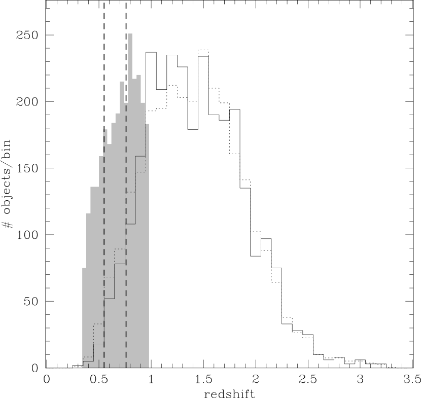
Figure 1.— Left panel: redshift distributions of MgII absorbers with $W_{0}>0.8\mathrm{\AA}$ used in this analysis (shaded histogram), of their background quasars (solid line) and of the complete population of reference quasars (dashed line). The latter is rescaled by a factor 4 to allow a direct comparison with the population of absorbed quasars. The vertical dashed lines mark the boundaries between the three bins in absorbers’ redshifts. Right panel: distribution of absorber rest equivalent widths. The vertical dashed lines separate the three bins in absorption strength.

All QSO spectra from the SDSS DR4 database (see Richards et al. 2002 for a definition of the SDSS QSO sample, also Schneider et al. 2005) were analyzed, regardless of QSO magnitude. The continuum-normalized SDSS QSO spectra were searched for MgII $\lambda\lambda 2796,2803$ doublets using an optimal extraction method employing a Gaussian line-profile to measure each rest equivalent width $W_{0}$. All candidates were interactively checked for false detections, a satisfactory continuum fit, blends with absorption lines from other systems, and special cases. The identification of Mg II doublets required the detection of the $\lambda 2796$ line and at least one additional line, the most convenient being the $\lambda 2803$ doublet partner. A 5$\sigma$ significance level was required for all $\lambda 2796$ lines, as well as a $3\sigma$ significance level for the corresponding $\lambda 2803$ lines. Only systems 0.1c blueward of the quasar redshift and redward of Lyman $\alpha$ emission were accepted. For simplicity, systems with separations of less than 500 km/s were considered as a single system. We note that MgII absorption lines are in general saturated, and in these cases no column density information can be directly extracted from $W_{0}(\lambda 2796)$. Given the typical S/N of SDSS quasar spectra, most of the detected MgII absorption lines have $W_{0}>0.8\;\mathrm{\AA}$. Weaker systems can occasionally be detected in the spectra of bright quasars but are significantly less numerous. As our technique requires a large number of absorbers we will only consider the stronger ones, i.e., $W_{0}>0.8\;\mathrm{\AA}$.

In this sample, multiple absorbers detected in the same quasar spectrum are found in $\sim 15\%$ of the systems. In order to ease the interpretation of our analysis, we select quasars with only one strong absorber detected in their spectrum. Finally, we restrict our analysis to MgII systems with $z<1$. After excluding a few tens of QSOs for which poor imaging data is available (mainly because of very bright saturated stars close by), the sample of absorbed QSOs includes 2844 objects. Their properties are summarized in Figure 1: the left panel shows the redshift distribution of the selected sample of MgII absorbers (shaded histogram) and their background quasars (solid line). The right panel presents the distribution of absorber rest equivalent widths.

2.2. Reference QSOs

In order to use a control sample in our analysis we need to select a population of quasars without absorbers. A number of criteria must be applied to ensure the selection of an unbiased sample: the two quasar populations must have the same redshift and apparent magnitude distributions, and must present the same absorption-line detectability. The selection of the reference quasar population is therefore defined as follows: for each quasar with a detected absorber with rest equivalent width $W_{0}$ and redshift $z_{abs}$, we randomly look for a quasar without any detected absorber above $W_{0}(\lambda 2796)=0.8\,$Å such that:

• they have similar redshifts: $\Delta z<0.1$;

• their magnitudes do not differ significantly: $\Delta m_{i}<0.5$;

• the absorption line is detectable in the reference spectrum, i.e., the S/N of the reference spectrum at the corresponding wavelength is high enough to detect the MgII $\lambda 2796$ line at the required level of significance. Such a requirement translates into $W_{min}(QSO_{ref},z_{abs})<W_{0}$, where $W_{min}$ is the minimum equivalent width that can be detected by the line finder at the corresponding wavelength.

The quasars selected in this way are called reference quasars in the following. Our selection procedure ensures that if similar absorbers were present in front of the selected reference quasars, we would have been able to detect them. In order to improve the noise properties of our analysis we select four independent reference quasars for each quasar with an absorber, resulting in a total of 11,376 objects.

2.3. Definition of absorbers sub-samples

The complete sample of MgII absorbers used in this study spans a large range in $z_{abs}$ (from 0.37 to 1.00), where substantial wavelength shift occurs. In fact, at the lowest redshift, $z_{abs}=0.37$, the 4000Å break feature lies in the observed $r$-band, whereas at $z_{abs}=1.00$ it occurs in the observed $z$-band. Moreover, the distance modulus between $z_{abs}=0.37$ and $z_{abs}=1.00$ increases by 2.6 mag, thus making low-$z_{abs}$ absorbing galaxies the dominant sources of signal in the overall stack. Therefore, in the following analysis we will consider three $z_{abs}$ bins: $0.37\leq z_{abs}<0.55$ (“low-redshift” sub-sample), $0.55\leq z_{abs}<0.76$ (“intermediate-redshift”), and $0.76\leq z_{abs}<1.00$ (“high-redshift”). The boundaries of this binning in $z_{abs}$ are indicated by the vertical dashed lines in the left panel of Figure 1. Possible dependence of the photometric and spatial properties on the absorption strength will be investigated by further splitting each $z_{abs}$ subsample into three different $W_{0}(\lambda 2796)$ subsamples: $0.8\mathrm{\AA}\leq W_{0}<1.12\mathrm{\AA}$ (“low-$W_{0}$” systems), $1.12\mathrm{\AA}\leq W_{0}<1.58\mathrm{\AA}$ (“intermediate-$W_{0}$” systems), and $W_{0}\geq 1.58\mathrm{\AA}$ (“high-$W_{0}$” systems). The boundaries of these bins are also shown as vertical dashed lines in the right panel of fig. 1. Finally, it is important to note that very strong systems ($W_{0}\gtrsim 3$Å ) are not expected to contribute significantly to our results as they are substantially less numerous than weaker ones.

3. Image processing and stack photometry

As indicated above (see also Zibetti et al., 2005a), our approach makes use of the fact that the galaxies linked to an absorbing system statistically produce an excess of surface brightness (SB) around the absorbed QSOs with respect to unabsorbed ones. Such a SB excess can be measured to obtain both global photometric quantities for the absorbing galaxies in different bands and the spatial distribution of the light of the absorbing galaxies, from which the impact parameter distribution of absorbing gas clouds can be derived.

In this section we describe the techniques that allow us to optimally integrate and measure the flux distribution of all and only the galaxies that cross-correlate with the presence of an absorber. By “optimally” we mean that any source of noise is minimized. In this measurement we are faced with three main sources of noise: (i) the intrinsic photon noise, which is fixed by the number of stacked images and their depth, (ii) the “background” signal produced by stars and galaxies which are not correlated with the absorbers, and (iii) the light from the QSO itself. While the intrinsic photon noise appears to be sufficiently low for a few hundred SDSS images and absorbers up to $z=1$ or more, the signal from background sources and the brightness mismatch which is allowed between absorbed and reference QSOs, although small, produce a noise which is orders of magnitude larger than the signal to be detected. These two sources of noise must be drastically reduced by applying accurate masking and QSO/Point Spread Function (PSF) subtraction algorithms on each image as described in the next two sections §§3.1 and 3.2.

The stacking and subsequent photometric analysis is conducted simultaneously in the four bands for which most of the flux is expected, i.e. $g$, $r$, $i$, and $z$. We use the so-called SDSS “corrected frame” images (fpC’s), which are bias subtracted and flat-field corrected, but preserve the original background signal. The error computation takes into account not only formal photometric uncertainties, but also sample variance and error correlation between different quantities in different bands. This is described in detail in §3.3.

3.1. Masking algorithm

The goal of the masking algorithm is to mask out any region of the image frame where flux is contributed by sources that have negligible probability of being a galaxy at the redshift of the absorber, $z_{abs}$. As a preliminary step, the light of the QSO is removed from a working copy of the image. This is done by subtracting the so-called postage-stamp image of the QSO output by the SDSS PHOTO pipeline (Lupton et al., 2001), in which the QSO is optimally de-blended from all surrounding sources. SExtractor (Bertin & Arnouts, 1996, V.2.3.2) is then run on the QSO-subtracted image to obtain a segmentation image and a catalogue of all sources detected $1\sigma$ above the local background over a minimum area of 10 pixels. The SExtractor’s segmentation image is used as base for the final mask. Only segments (i.e., groups of pixels) attributed to sources that are too bright to be a galaxy at $z_{abs}$ are kept in the mask.

For the mask thresholds, we adopt the fluxes derived for an unobscured, metal poor stellar population produced in a 10 Myr long burst, observed right after the end of the burst itself, with rest-frame $g$-band absolute magnitude $M_{g,\mathrm{threshold}}=-22.4~{}\mathrm{mag}$ (as computed by the code of Bruzual & Charlot, 2003), observed at $z_{abs}$. The flux-limited masks are computed separately in $g$-, $r$- and $i$-band, that roughly correspond to the rest-frame $g$- and $u$-bands in the redshift range spanned by the absorbers in our sample. The choice of this very “blue”, UV-bright SED is motivated by the need to avoid the exclusion of UV-bright galaxies, while keeping the flux thresholds relatively low in order to minimize the contamination by bright interlopers. Compared to the field luminosity function (LF) in a similar redshift range (cf. Gabasch et al., 2004), our flux thresholds are $\sim 1$ mag brighter than $M^{\star}$ in the rest-frame $g$-band, and $\sim 1.8$ mag brighter in $u$. We make sure that the exclusion of galaxies at the very bright end of the LF does not affect our results by performing the stacking using a more conservative value of $M_{g,\mathrm{threshold}}=-23.9~{}\mathrm{mag}$ (i.e. 1.5 mag brighter than previously assumed). While the noise from bright interlopers increases significantly, no systematic effect results from this change in the masks. Therefore, all the analysis of this paper is conducted on images masked with $M_{g,\mathrm{threshold}}=-22.4~{}\mathrm{mag}$. For illustration, we plot the apparent $r$-band threshold magnitude as a function of the absorber’s redshift (solid line) in Figure 2. The dotted line displays the magnitude of a $M_{g}=M_{g}^{\star}$ galaxy for an intermediate (Sbc) SED template. The choice of a UV-bright template yields flux thresholds that become increasingly brighter than “normal” $M_{g}^{\star}$ galaxies at increasingly higher redshift.

It is worth noting that at low redshift some absorbing galaxies can possibly be detected in the SDSS images: in fact, the SDSS photometric sample has a completeness larger than 95% (for point sources) at $r<22.2$ mag and thus would allow to detect objects as faint as $M_{g}=M_{g}^{\star}$ up to $z=0.65$, and 10 times fainter than that at $z=0.37$ (an analysis of galaxy number counts will be presented in a forthcoming paper). However, at $z_{abs}\gtrsim 0.7$ the detection of individual galaxies is completely precluded and only the stacking technique is able to reach the required sensitivity.

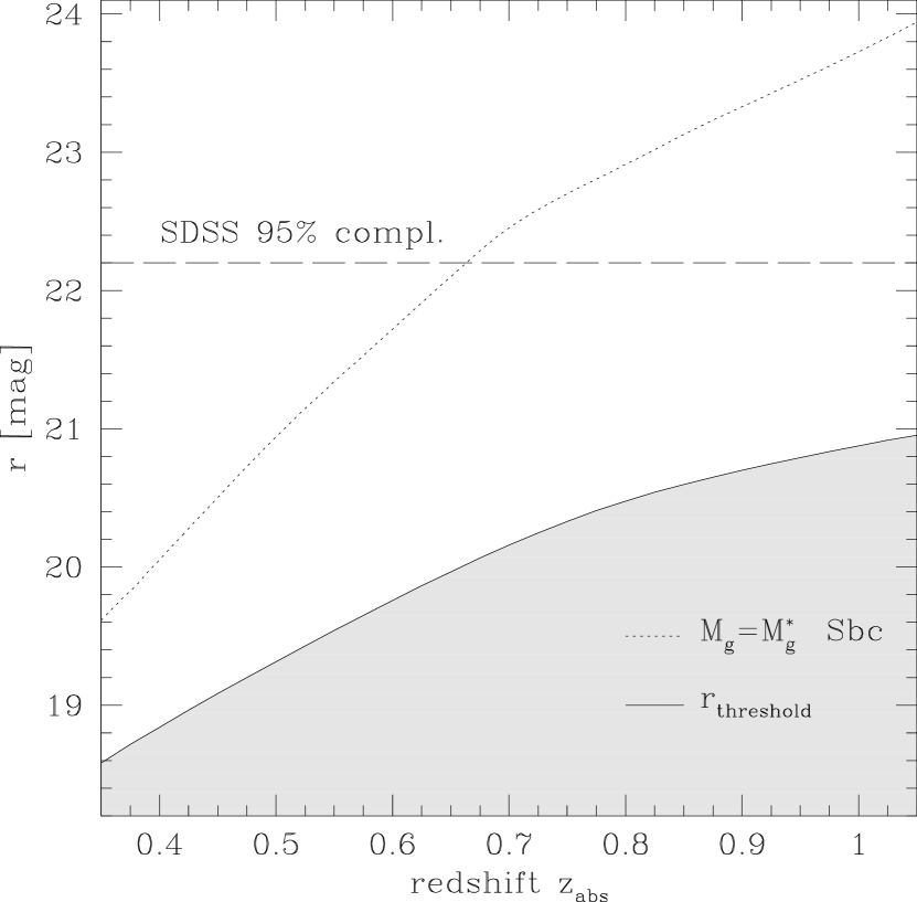
Figure 2.— The threshold magnitude for the masks in $r$-band as a function of the absorber’s redshift $z_{abs}$ (solid line), compared to the apparent magnitude of a “normal” (Sbc SED template) $M_{g}=M_{g}^{\star}$ galaxy (dotted line). The horizontal long dashed line is the magnitude where completeness of the SDSS photometric catalog drops below 95% (point sources).

In the second step, we build a mask where all stars brighter than 21.0 mag in $r$ are covered with a circular patch of radius $R=1.2\times a_{25}+3$ (in pixels), where $a_{25}$ is the median of the isophotal semi-major axis at 25 mag arcsec^-2 in $g$, $r$, and $i$. For saturated stars, $a_{25}$ is replaced by three times its value, in order to avoid the extended halos of scattered light that surround these stars. For this step we entirely rely on the SDSS-DR4 photometric catalogs (PhotoPrimary table) in order to ensure optimal star/galaxy separation (see Ivezić et al., 2002).

Finally, the flux-limited masks in the three bands and the star mask are combined into a final mask, where a pixel is masked if and only if it is masked in any of the input masks (logical or).

3.2. QSO’s PSF subtraction

In very high S/N images, like the stacked images, the spread light of a QSO can be detected out to angular distances of a few tens of arcsecond and still contribute a non-negligible fraction of the azimuthally averaged SB linked to the absorbers. In order to suppress this contribution with the best possible accuracy, the SB distribution of the QSO is estimated from the high S/N PSF of bright, unsaturated stars. More specifically, for each QSO we look for a star that fulfills the following requirements. (i) The star must not be saturated, nor fainter than 17 mag ($r$ band); stars with interpolated pixels, cosmic rays, or flagged for any photometry defect are rejected, as well as those stars whose centers happen to lie less than 5 pixels apart from any mask in the frame (see below how PSF star frames are masked). (ii) The star must have been observed during the same run as the QSO, in the same SDSS camera column, and within 10 arcmin angular separation from the QSO. These two criteria, (i) and (ii), ensure that the PSF is photometrically accurate and it is taken in observing conditions that are consistent with those of the QSO. Among the stars selected in this way, the one that best matches (iii) the size (as determined by the second moment of the light distribution) and colors ($g-r$ and $r-i$) of the QSO is chosen as representative of the QSO’s PSF. This last selection aims at minimizing the effects of the space/time and color dependence of the PSF. In fact, it must be noted that QSOs are on average bluer than stars and therefore, have broader PSFs at any given position, on average. The selection at point (iii) minimizes this effect and, at the same time, compensates for it by exploiting the spatial variation of the PSF. The stars selected to model the PSF have median $r\sim 15.7$ mag, and span the range between 13.4 and 17 mag. The median difference in color between QSOs and the corresponding stars is $-0.28$ mag (rms 0.21) in $g-r$ and $-0.06$ mag (rms 0.16) in $r-i$. The distribution of difference in size is centered at 0, with 0.16 pixels rms.

The masking algorithm described above (§3.1) is then applied to each selected reference star; however, no lower flux threshold is applied and all SExtracted sources are retained in the masks. The subtraction of the PSF frame from the QSO frame is only possible for pixels that are unmasked in both frames. Thus, in order to limit the loss of effective detection area around the QSOs, we “restore” as many as possible masked pixels in the PSF frame in the following way. The PSF frame is virtually divided into four quadrants centered on the reference star. Each masked pixel is then replaced by the average of all (if any) unmasked pixels at axisymmetric positions in the other three quadrants. If none of the symmetric pixels is unmasked, the pixel is kept masked. This “symmetrization” process is very effective and results in no more than 0.05% of the area masked in 95% of the PSF frames.

The normalization of the PSF to the QSO, necessary before the subtraction can be done, is computed using the PSF magnitudes from the SDSS-DR4.

3.3. The stacking and photometry procedures

Before all images are actually stacked, we rescale them to the same physical scale at the redshift of the absorber, $z_{abs}$. This is determined such that at the lowest redshift, $z_{abs}=0.37$, the original SDSS pixel scale is preserved (0.396 arcsec pixel^-1); the resulting common pixel scale is thus 2.016 kpc pixel^-1. Pixel intensity is accordingly rescaled in order to conserve the total flux in any object. The images of reference QSOs are rescaled according to the redshift of the absorber in the corresponding absorbed QSO. PSF stars are rescaled with the same geometry as their corresponding QSO.

As individual images contribute to the final stacked image only with their unmasked regions, it is mandatory that all images are accurately background subtracted to avoid spatial background fluctuation in the final stacked image that might strongly reduce the photometric accuracy. A constant background level in each image (QSOs and stars) is computed as the median of the unmasked pixel values within an annulus between 400 and 500 kpc. Two $\sigma$-clipping iterations with $\pm 3\sigma$ cut are performed to exclude the faint sources that are left unmasked by the masking algorithm (see above, §3.1).

All images are also intensity rescaled in order to match a common photometric calibration (according to the SDSS photometric standard defined by Fukugita et al., 1996; Smith et al., 2002), that includes the correction for Galactic extinction. More specifically, the calibrated pixel intensity $I_{calib}$ is derived from the raw pixel intensity in the fpC $I_{raw}$ according to the following equation:

$$I_{calib}=I_{raw}\cdot\frac{f_{20,\mathrm{ref}}}{f_{20}}\cdot 10^{0.4\cdot A_{\lambda}}$$ (1)

where $f_{20}$ and $f_{20,\mathrm{ref}}$ are the pixel counts corresponding to 20 mag (observed) in the fpC original frame and in the final reference photometric system, respectively. $A_{\lambda}$ (in mag) is the galactic attenuation in the working pass-band, computed from the Schlegel et al. (1998) dust distribution map.

The final stacked image in each band, for any given sample of QSOs (either absorbed or reference), is computed such that the resulting intensity at any pixel is the simple average of the net PSF-subtracted counts over all corresponding pixels which are unmasked in the individual images:

$$I_{stacked}=\frac{\sum_{i=1}^{N}mask(i)\times(I_{QSO,i}-I_{PSF,i})}{\sum_{i=1}^{N}mask(i)}$$ (2)

where $I_{stacked}$ is the intensity of a given stacked pixel, $I_{QSO,i}$ and $I_{PSF,i}$ are the calibrated, background-subtracted intensities of the QSO and PSF frames at the corresponding pixel in the $i^{th}$ image, and $mask(i)$ equals 1 if the pixel is unmasked in both the QSO and the PSF image, 0 otherwise. It is worth mentioning that, at a given position on a stack image, only 6 to 11% of the individual images are masked in the low-$z_{abs}$ bin and even less at higher redshift. The final intensity, $I_{stacked}$, is therefore a reliable estimate of the average value. A careful re-determination of the (residual) background level is done on the final stacked image in an annulus between 350 and 500 kpc. Circular aperture photometry is then performed, by simply averaging the pixel intensities in a series of circular annuli.

For the purpose of determining uncertainties that take into account not only formal photometric errors, but also the effects of sample variance and the correlation between different apertures and bands, the full covariance matrix is computed by means of a jackknife algorithm. For any given subsample of $N$ QSOs, the stacking and photometric measurements in the four bands are repeated $N$ times, leaving out a different QSO each time. The covariance matrix of the aperture photometry fluxes obtained from these $N$ realizations is then multiplied by $N-1$ to give the sample covariance matrix. All the errors relative to the photometric quantities derived from the primary aperture fluxes, such as integrated fluxes, colors, and profile shape parameterizations, are computed using this covariance matrix.

Absorbed and reference QSOs are stacked and analyzed separately as far as primary aperture photometry is concerned. However, all the results that will be presented and discussed in the following sections are obtained from net (i.e., absorbed$-$reference QSOs) aperture photometry. For the error estimates of the derived quantities, absorbed and reference QSOs are treated as independent datasets, thus the combined covariance matrices have null cross terms. We note that this assumption is correct only as a first order approximation; as we will discuss below in §4.1 and Appendix A, there are systematic effects in the stacked reference QSOs that depend on the redshift and magnitude of the QSO, thus making the absorbed and reference samples correlated. Neglecting such second-order error correlation results in slightly over-estimating errors on the final net photometry, especially within the seeing radius (i.e., the radius that corresponds to the FWHM of the PSF image).

All the stacking and photometric measurements described in this subsection and in the following sections are performed using a dedicated package of programs and utilities, which are developed in C language by S.Z. The package relies on the cfitsio libraries (Pence, 1999) for input/output interface and makes use of a number of Numerical Recipes routines (Press et al., 1992). The analysis presented in this paper results from the processing of 0.5 Terabyte of imaging data.

4. The spatial distribution of MgII absorbing galaxies

In this Section we present an analysis of the surface brightness distribution of the excess light around absorbed QSOs and infer from that the spatial distribution of absorbing galaxies with respect to the MgII systems probed by the QSOs sight-lines. In particular, in §4.1 we present the SB profiles extracted from the stack images, and parameterize their shape as a function of the absorption rest equivalent width, $W_{0}(\lambda 2796)$, and absorption redshift, $z_{abs}$. In §4.2 we will show that the SB profile is directly related to the impact parameter distribution weighted by the luminosity of the absorbing galaxy. Such a distribution will be explicitly derived and discussed in §4.3.

4.1. Stack images and surface brightness profiles

In Figure 3 we report an example of typical final stack images for the absorbed QSOs (left panel) and for the corresponding control sample of reference QSOs (right panel). More specifically, this is the $r$-band stack for the low $z_{abs}$ sample that includes all $W_{0}$. The two panels reproduce a region of 600$\times$600 kpc² projected at $z_{abs}$, centered on the QSOs. The grey level intensity maps the surface brightness linearly. The corresponding levels, expressed in physical units of apparent magnitudes per projected kpc², are indicated by the vertical color bar between the two panels. The infinity level ($\infty$) indicates the background signal.

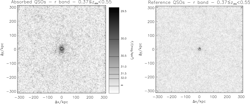
Figure 3.— The $r$-band stack images of absorbed (left panel) and corresponding reference QSOs (right panel) in the redshift range $0.37\leq z_{abs}<0.55$. The sample of reference quasars is four times larger which results in a lower noise level. Both images are PSF-subtracted and are visualized with the same color scale, as indicated by the color bar marked in units of magnitudes per kpc² ($\infty$ corresponds to the background level). The excess of light around the absorbed QSOs is apparent.

In both panels, we note that the intensity of the very central pixels is zero, within the typical background noise uncertainties. This is obtained by construction, by subtracting the PSF from each individual stacked image. The fact that these central pixels are zeroed to such high accuracy is indicative of the good quality of our PSF subtraction algorithm. What is most important to notice in Figure 3 is the SB excess around the QSOs, beyond the very central pixels. Although an excess is seen in both panels, it is apparent that the SB excess around absorbed QSOs is much more intense and extended than around the reference QSOs; it can be seen, even by eye, that the excess around the absorbed QSOs extends well beyond 50 kpc, whereas nothing is apparent around the reference QSOs beyond 10-15 kpc. This effect is even more significant if one considers that the reference QSO image results from 4 times as many QSOs as in the absorbed QSO image (see §2.2), and therefore has twice as low background noise.

The SB excess observed around the reference QSOs is a systematic effect which is mainly caused by the emission of the QSO’s host galaxy/environment. We analyze the origin of this effect in greater detail in appendix A. Regarding the measurement of the light of absorbing galaxies, we can treat the SB excess found around reference QSOs as a pure systematic additive contribution, which is inherent to any subsample of QSOs with a given redshift and magnitude distribution. Therefore, for each subsample of absorbed QSOs, the final stack image (SB profile) of the corresponding reference QSOs is subtracted from the absorbers’ one to obtain a net image (SB profile).

Next we analyze the SB distribution of the galaxies responsible for the MgII absorption by extracting one-dimensional SB profiles from circular annuli, within which the average SB is computed. The spacing between subsequent apertures is chosen to ensure adequate S/N in all apertures; this results in a progression that increases slightly faster than a geometric one.

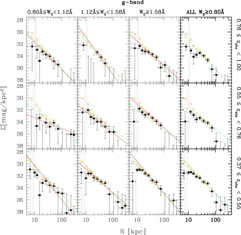
Figure 4.— The $g$-band surface brightness profiles of the light around absorbed QSOs, in different bins of redshift $z_{abs}$ (indicated by the labels on the right-hand side) and rest-frame equivalent width of the 2796Å line (labels along the top of the figure). Black filled dots with error bars represent the net SB, i.e., after subtracting the residual systematic contribution measured from the reference QSOs inside 50 kpc. The orange open circles with error bars show the SB prior to the subtraction of the SB of the reference sample. The dashed green line is the same in all four panels of each row, and displays the best power-law fit for the sample including all $W_{0}(\lambda 2796)$ in that $z_{abs}$ bin. The power-law fits for the three $W_{0}(\lambda 2796)$ subsamples in each redshift interval are shown by the red solid lines. In each panel, vertical dotted lines mark the distance corresponding to the 1.4″ average seeing (FWHM) at the minimum and maximum redshift in the subsample.

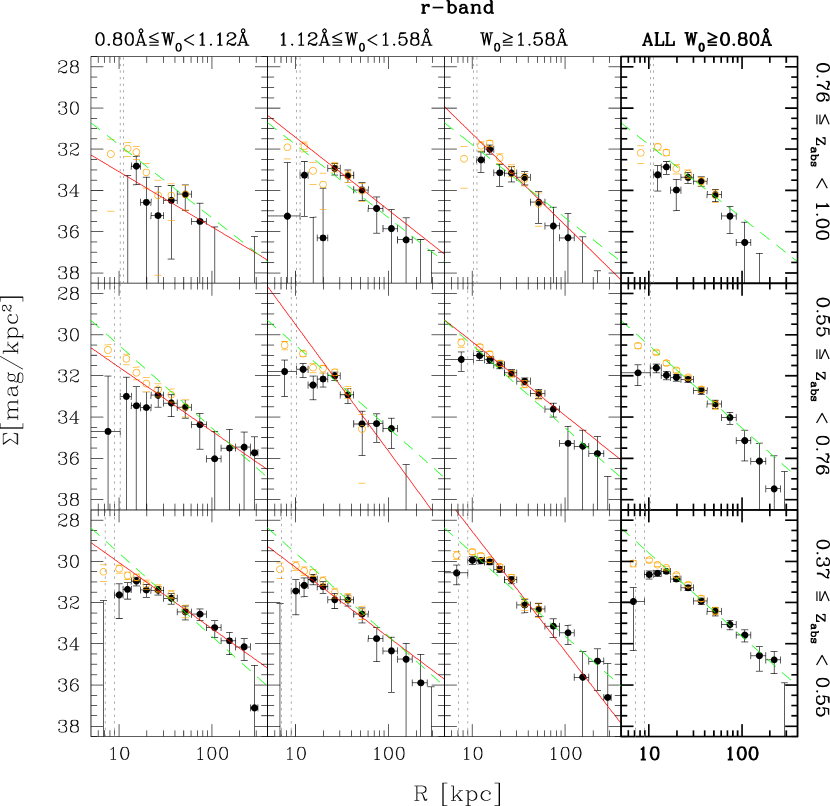
Figure 5.— Same as Figure 4, but for the $r$-band.

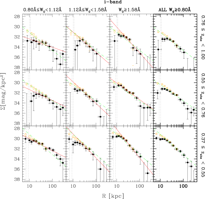
Figure 6.— Same as Figure 4, but for the $i$-band.

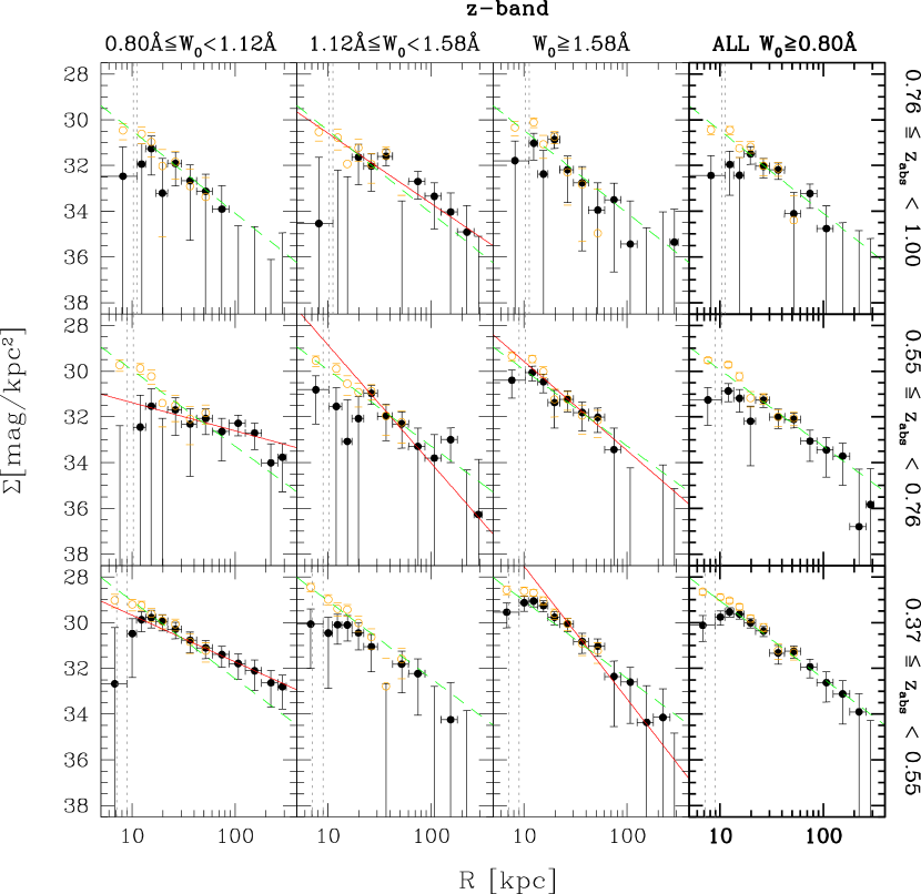
Figure 7.— Same as Figure 4, but for the $z$-band. Note that for three out of the nine $W_{0}$ subsamples no power-law fits (red lines) are reported, because the large uncertainties make the fit meaningless.

The SB profiles of the absorbers in all our subsamples are presented in Figures 4 to 7, for the $g$, $r$, $i$, and $z$ band, respectively. Each of these figures is organized in twelve panels: three rows corresponding to the three $z_{abs}$-bins (from the lowest in the bottom row to the highest in the top one), and four columns for the low-, intermediate- and high-$W_{0}$ systems, plus the total of the $z_{abs}$-bin (“all”), from left to the right. The impact parameter $R$ is reported on the x-axis in logarithmic scale, while the surface brightness is given on the y-axis in units of apparent magnitudes per projected kpc². The net SB profile is shown by the black filled dots with error bars. Vertical error bars represent the jackknife estimate of the SB uncertainty computed as above (§3.3), while the horizontal error bars just mark the width of the radial bin. The orange open circles with upper and lower ticks indicate the uncorrected SB determination and relative jackknife uncertainty, prior to the subtraction of the systematic excess measured from the reference QSOs sample. It must be noted that beyond 50 kpc no subtraction is performed (hence no orange points) as the reference stack images are completely consistent with zero at this impact parameter, and the subtraction would just increase the noise in the net profile.

As a preliminary sanity check, we note that the signal decreases from the lowest to the highest $z_{abs}$ bin by roughly 2 mag, which is consistent with the cosmological dimming expected for the covered redshift range. The first important result that we can extract from Figures 4 to 7 is that there is light that cross-correlates with the MgII absorbing clouds out to 100-200 kpc projected distance. This clearly indicates that MgII absorption systems probe the intergalactic medium out to quite large galactocentric distances, and may possibly arise in complex galaxy environments.

It must be noted that the PSF subtraction artificially introduces the constraint $\mathrm{SB}=0$ within the first resolution element (corresponding to the seeing). In Figure 4, the two vertical short-dashed lines in grey reported in each panel show, at the lowest and highest $z_{abs}$ in the bin, the value of 1.4″ which corresponds to the median seeing (FWHM) in SDSS images. Due to the above normalization we expect the signal to be strongly decreased within this radius ($\sim 10$kpc), and significant deviations from the “true” SB profile to occur out to twice this distance from the QSO ($\sim 20$kpc) as a result of the breadth of the seeing distribution in our images.

The SB profiles between $R=20$ kpc and $R=100$ kpc in all bands are generally well approximated by a single power-law with index ranging from $-1$ to $-2.5$. Between 10 and 20 kpc (roughly corresponding to one to two times the median seeing value at all redshifts) we observe a break and a deficit with respect to the powerlaw, which can be mostly ascribed to the central normalization. However, real departures from a powerlaw profile in the inner 20 kpc cannot be excluded based on the present analysis. Also, it is worth noting that previous studies show that very few galaxies, if any, are associated with MgII absorbers at impact parameters $<10$ kpc (Steidel et al., 1994; Churchill et al., 2005a). Thus the signal that we miss from the central part of the profile is probably negligible. Beyond 100 kpc the photometric uncertainties are too large to derive any reliable information about the profile shape, although significant detections are obtained in several bands and bins.

Power-law fits of the form

$$S(R)=S(\overline{R}){\left(\frac{R}{\overline{R}}\right)}^{\alpha}$$ (3)

are performed in the impact parameter range $20~{}\mathrm{kpc}<R<100~{}\mathrm{kpc}$ by minimizing the $\chi^{2}$ computed using the full data covariance matrix. The slopes, $\alpha$, for each absorber bin are reported in Table 1 (columns 2-5, for each band respectively), along with their upper and lower confidence limits (1-$\sigma$), which are obtained from the 2-dimensional $\chi^{2}$ distribution in the $S(\overline{R})-\alpha$ parameter space. Column 6 reports the weighted average of the slopes in the four bands, with relative error. The best fitting power-laws are also shown in the panels of Figure 4 to 7. They are shown in red for the three EW bins and with a dashed green line for the “All”-EW panels. The fit to the “All”-EW sample is also reported as a dashed green line in all other panels to facilitate a prompt comparison between different subsamples.

Looking at the “All”-EW samples we observe that, within the quoted uncertainties, all profiles in the four observed bands and in the three redshift bins are consistent with a common slope, $\alpha$, between $-1.4$ and $-1.6$. There is no evidence for any redshift evolution of the power-law slope for the average SB distribution of absorbers related galaxies between $z_{abs}=0.37$ and 1. This is confirmed and better constrained by the weighted average of the slopes in the four bands reported in column 6 of Table 1: their values are consistent within 1-$\sigma~{}(\leq 0.17)$ among the three $z_{abs}$ bins.

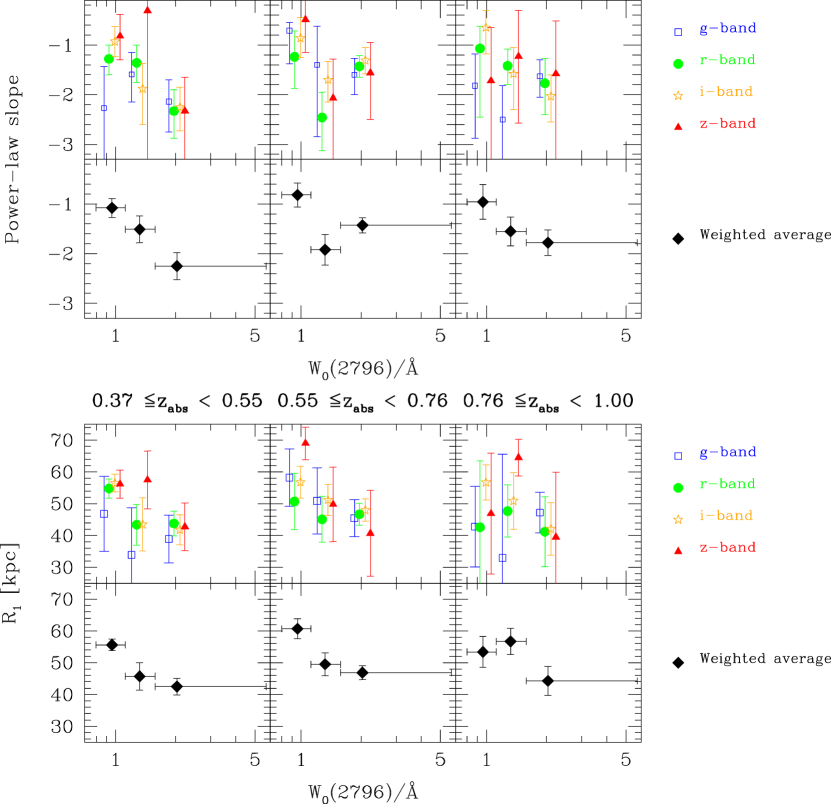
Figure 8.— The correlation between the shape of the surface brightness profiles and the absorption strength. In the top panels, the slope of the best fit powerlaw slope ($20~{}\mathrm{kpc}<R<100~{}\mathrm{kpc}$) is plotted against the absorption strength, for the three $z_{abs}$ bins, as indicate by the labels in the middle. Blue open squares, green filled circles, orange empty stars, and red filled triangles are shown in the upper row for the $g$-, $r$-, $i$-, and $z$-band respectively. The black filled diamond in the lower row is the weighted average of the four bands. The horizontal error bars show the extent of each EW bin. The bottom panels are the same as the top ones, but for the first moment of the SB distribution $R_{1}$ (see text).

A second interesting result that emerges from Figure 4 to 7 can be derived by comparing different EW bins, especially in the most sensitive $r$ and $i$ bands for the low-$z_{abs}$ systems. It is apparent that the high-$W_{0}$ MgII systems have systematically steeper power-law profiles than the weaker systems. Despite the relatively large uncertainty of our slope measurements, this trend is clear in the low-$z_{abs}$ bin from the values reported in Table 1. We also plot these values in the top panels of Figure 8, where different symbols represent the measurements in the four bands as a function of the absorption strength, binned as defined in §2.3. The three columns of panels are for the three $z_{abs}$ bins. The large filled diamonds in the lower row represent the weighted average of the four bands, while the values for the different bands are shown in the upper row. At the lowest $z_{abs}$ the trend of steepening of the profile with absorption strength is unambiguously detected in $r$ and $i$ and statistically confirmed by the weighted averages. The power-law slope steepens from $-1.1$ in the weakest systems, to $-2.3$ in the strongest. Similar trends (in particular for the weighted averages) are seen at higher redshift too.

We further investigate the systematic variation of the surface brightness profiles as a function of the absorption strength in a model independent, non-parametric way, by means of the first moment of the SB distribution in $R$. This is defined as:

$$R_{1}=\frac{\int\limits_{10~{}\mathrm{kpc}}^{100~{}\mathrm{kpc}}S(R)~{}R^{2}~{}dR}{\int\limits_{10~{}\mathrm{kpc}}^{100~{}\mathrm{kpc}}S(R)~{}R~{}dR}$$ (4)

$R_{1}$ is thus given in kpc and can take any value between 10 and 100 (see above in this section why 10 kpc is chosen as lower limit). As we will demonstrate in the next §4.2, $R_{1}$ can be interpreted as the luminosity-weighted average impact parameter of MgII absorbing galaxies. Small values of $R_{1}$ characterize centrally concentrated light profiles, while less concentrated profiles have larger $R_{1}$. The values of $R_{1}$ computed for the four bands and their statistical errors are reported in columns 7 to 10 of table 1, for all bins; the weighted average among the four bands is reported in column 11. We note that $R_{1}$ is remarkably constant among different redshift. For “All” EW $<R_{1}>$ is 48 kpc. However, for strong systems this value decreases to 43 kpc (at low-$z_{abs}$, similar at higher redshift) while it approaches 60 kpc for the low-$W_{0}$ systems. As for the power-law index, we also plot these values in fig. 8 (bottom panels). Again, these plots confirm that stronger systems have more centrally concentrated profiles. The effect appears statistically significant at low and intermediate $z_{abs}$, especially when the weighted average of the four bands is considered. For the highest redshift bin the trend is much more uncertain because of the lower S/N, but is still consistent with the lower redshift samples.

4.2. From surface brightness profiles to the impact parameter distribution of MgII systems

In this section we provide a derivation of the link between the surface brightness profiles obtained from the stacked images and the impact parameter distribution of the MgII absorbing clouds. First, we demonstrate that if each MgII absorber is linked to only one galaxy, then the SB at any radius $R$ is proportional to the luminosity weighted impact parameter distribution.

Let us consider initially the case of galaxies with fixed luminosity $\bar{L}$, surrounded by MgII absorbing clouds resulting in a probability of producing an absorption along the sight-line

$$dP(R,\bar{L})=p(R,\bar{L})~{}dA,$$ (5)

where $p(R,\bar{L})$ is the differential probability per unit area at given luminosity $\bar{L}$, which we assume to be independent of position angle. Although this assumption might not be verified for single galaxies, it is always automatically realized in the case of stacked images. Let us now consider a set of QSOs homogeneously distributed in sight-lines around $\bar{L}$ galaxies. The number of QSOs that are actually absorbed at given impact parameter $R$ is thus given by

$$dN_{abs}(R,\bar{L}) = N_{abs}(\bar{L})~{}dP(R,\bar{L})$$ (6)

$$= 2\pi N_{abs}(\bar{L})p(R,\bar{L})~{}R~{}dR,$$ (7)

where $N_{abs}(\bar{L})$ is the total number of QSOs with detected absorption. If we now stack all the absorbed lines-of-sight, we find the azimuthally averaged surface brightness:

$$SB(R,\bar{L})=\frac{dN_{abs}(R,\bar{L})\cdot\bar{L}}{2\pi~{}R~{}dR\cdot N_{abs}(\bar{L})}.$$ (8)

This is valid in the limit that the effective extent of each galaxy is significantly smaller than $R$. As galaxies with $L\sim L^{\star}$ have typical effective radii of the order of 3 kpc, at $R\gtrsim 10$ kpc Equation 8 is a fair approximation. Substituting Equation 7 into this expression we see that the area from the probability cancels out with the normalization of the azimuthal average and we have

$$SB(R,\bar{L})=\bar{L}\cdot p(R,\bar{L})\,.$$ (9)

Therefore, the SB profiles presented in the previous figures are directly proportional to the probability of producing absorption at a given distance from a galaxy. If we now consider contributions from galaxies of different luminosities, we can write

$$SB(R)=\int L~{}\frac{dp(R,L)}{dL}~{}dL,$$ (10)

that is to say that the SB at any radius $R$ is proportional to the luminosity-weighted impact parameter distribution.

In order to take into account the effect of satellite galaxies, or environment if a MgII absorber is associated with more than one galaxy (for example in a group), we can extend the argument that leads to Equation 9. Let now $\bar{L}$ be the luminosity of the brightest associated galaxy and $R$ measure the impact parameter from it. The presence of secondary galaxies increases the total luminosity per absorber and produces a spatially extended contribution to the average SB. By defining $K_{\bar{L}}(R)$ as the average surface brightness around the location of an $\bar{L}$ galaxy, including all its satellites and possible companions, and normalized dividing by $\bar{L}$, we can then rewrite Equation 9 as

$$SB(R,\bar{L})=C_{\bar{L}}\cdot\bar{L}\cdot(p(R,\bar{L})\otimes K_{\bar{L}}(R))$$ (11)

where the $C_{\bar{L}}$ accounts for the increased total luminosity per absorber and $p(\bar{L},R)$ is convolved with $K_{\bar{L}}(R)$. Finally, integrating over luminosity we obtain the analogous of Equation 10 for multiple associated galaxies

$$SB(R)=\int C_{L}\cdot L\frac{d(p(R,L)\otimes K_{L}(R))}{dL}~{}dL$$ (12)

It is immediately seen that this last equation simplifies to Equation 10 when $C_{L}=1$ and $K_{L}(R)=\delta_{\mathrm{Dirac}}(R)$ for every $L$, i.e., when there is only one associated galaxy per absorber, with negligible spatial extent.

4.2.1 How many galaxies per absorber?

Although the association of an individual galaxy with an absorber is a somewhat ill-defined procedure, in order to interpret the SB profiles and especially the SEDs, it is highly relevant to understand how many (bright) galaxies per absorber contribute to the cross-correlating light. Preliminary results by Ménard et al. (in preparation) indicate that at $z_{abs}<0.6$ there is on average one bright galaxy detected in excess within $\sim 100$ kpc around absorbed QSOs in comparison to reference QSOs. As we will show in §5, the average total luminosity $<C_{L}\cdot L>$ (within 100 kpc, in the low-$z_{abs}$ bin) is $m_{r}=-21.5~{}(\pm 0.2)$ or $\approx 2.8\times 10^{10}L_{\odot,r}$, corresponding to the $L^{\star}_{r}$ of the local field luminosity function in the SDSS by Blanton et al. (2003) (we adopt Blanton et al., 2005, to convert from magnitudes in the z=0.1 system to the rest-frame). If we compare this value to the LF at $z\sim 0.5$, then this luminosity corresponds to $0.5~{}L^{\star}$ (e.g. in COMBO-17, Wolf et al., 2003). Such a relatively low luminosity inside a 100 kpc circle shows that, on average, strong MgII absorbers with $0.8$Å $<W_{0}\lesssim 3$Å do not reside in dense galaxy environments. This statement however cannot be proved for stronger systems (with $W_{0}\gtrsim 3$Å) alone as their relative contribution to the signal is substantially lower.

Therefore, in the following we will interpret the SB profile $SB(R)$ to first order approximation as the luminosity weighted average probability of intercepting an absorber at a given impact parameter $R$ from a bright galaxy. Regarding the corresponding spectral energy distribution (SED), the inclusion of small companions and satellite galaxies in the integrated light is expected to have a minor influence on our estimates of total luminosity and spectral properties. In practice we will treat such properties as the properties of a single absorbing galaxy.

4.3. The impact parameter distribution of MgII absorbers

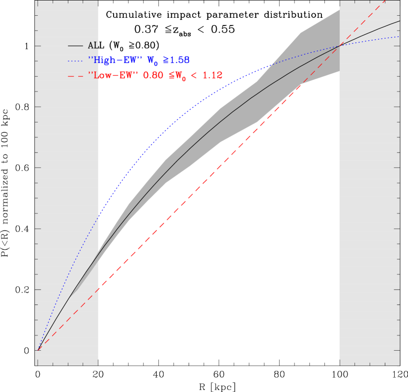
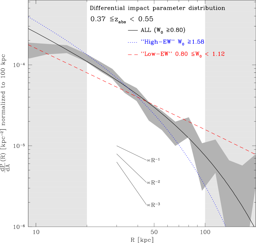
Figure 9.— Luminosity-weighted impact parameter distributions for the low $z_{abs}$ sample, normalized between 0 and 100 kpc. The left panel shows the cumulative probability of observing a galaxy at impact parameter $<R$ from an MgII-absorbed QSO (see Equation 13). The three lines are the $\tanh$ analytic fits to the distributions for all (black solid line), high-$W_{0}$ (blue dotted line), and low-$W_{0}$ (red dashed line) systems. The dark grey shaded area represents the 1-$\sigma$ confidence interval empirically derived from the photometry for the whole low-$z_{abs}$ sample. Data points in the regions shaded in light grey were excluded from the fit. The right panel reports the differential probability $\frac{dP}{dA}(R)$, as analytically derived from the cumulative one. Different line styles and shadings represent the same quantities as in the left panel. Three lines with different logarithmic slopes are also plotted for easy comparison.

Based on the arguments presented in the previous paragraphs, we translate the observed SB distributions around the absorbed QSOs into a luminosity weighted probability of intercepting an MgII-absorbing system at a given impact parameter from a galaxy. In differential form this is directly given by the SB profiles (see §4.1), modulo an arbitrary normalization factor. As already noted, simple power laws are able reproduce the SB profiles, and hence also the differential probability profiles, reasonably well. Here we introduce the integral form

$$P(<R)=\int\limits_{0}^{R}2\pi~{}R^{\prime}~{}dR^{\prime}\int L\frac{dp(R^{\prime},L)}{dL}dL$$ (13)

where $P(<R)$ is the luminosity weighted probability of measuring an impact parameter between 0 and $R$. This form of cumulative probability distribution is particularly useful for defining characteristic scale lengths. According to Equations 5 and 10, this is simply proportional to the apparent luminosity integrated between $0$ and $R$, $F(<R)$. The proportionality factor between the two distributions is just given by the total integral flux.

Observationally, however, we are faced to two limitations. At large radii small background uncertainties yield huge uncertainties in the estimate of the total integral flux. Therefore we are forced to limit the flux integral to an arbitrary large radius where the background level uncertainty is negligible. This is chosen as 100 kpc, which implies that the impact parameter distribution will be normalized to 1 between 0 and 100 kpc. The second limitation is that at small radii ($R\lesssim~{}10$-20 kpc) the finite size of the PSF does not allow a reliable estimate of the flux (see §4.1), and therefore we can produce flux growth curves only from 10-20 kpc outwards.

We overcome this problem by extrapolating the growth curve to $R=0$ using an analytic fit to the empirical growth curve. Only the conservative range between 20 and 100 kpc is used. As a convenient fitting function we choose an hyperbolic tangent generalized as follows:

$$F(R)=\alpha\tanh[\beta\cdot(R-\delta)]+\gamma$$ (14)

From this fit we can derive the (extrapolated) total flux between 0 and 100 kpc $F_{100}\equiv F(100)-F(0)$, and hence express

$$P(<R)=c_{1}\tanh[c_{2}\cdot(R-c_{3})]+c_{4},$$ (15)

where

$$c_{1}=\alpha/F_{100}$$ (16)

$$c_{2}=\beta$$ (17)

$$c_{3}=\delta$$ (18)

$$c_{4}\equiv c_{1}\cdot\tanh(c_{2}\cdot c_{3}).$$ (19)

The $i$-band photometry in the low-redshift sample is used to derive the cumulative impact parameter distribution $P(<R)$. Thus what we present here is weighted on the rest-frame $g$-band light. In table 2 we report the four coefficients of the analytic formula given in Equation 15 for several bins of $W_{0}$. These analytic expressions are meant to be handy representations for the $P(<R)$ extracted from a robust statistical analysis. No physical model is implied. However, the reader should be aware that below 20 kpc these formulae are extrapolated and that the normalization within 100 kpc is arbitrary.

In the left panel of Figure 9, $P(<R)$ is plotted for all EWs as a solid line. The dark grey shaded area is the 1-$\sigma$ confidence region for $P(<R)$ as it is directly derived from the $i$-band (roughly rest-frame $g$-band) flux growth curve of the entire sample at low redshift. The integral impact parameter distributions for the low- and high-$W_{0}$ systems are overplotted in the same panel with dashed red and dotted blue lines, respectively. Again, the higher concentration of stronger systems is evident. This is also quantified by the values of $R_{50}$ and $R_{90}$ reported in Table 2 that represent the distances from the “parent” galaxy within which the probability of finding an absorber system is 50 and 90% respectively (as computed from Equation 15).

Table 2Parameters of the impact parameter distribution $P(<R)$ ($0.37\leq z_{abs}<0.55$)

$W_{0}(\lambda 2796)$	$c_{1}$	$c_{2}$	$c_{3}$	$c_{4}$	$R_{50}$	$R_{90}$
		kpc-1	kpc		kpc	kpc
All	7.900	$7.275\cdot 10^{-3}$	$-163.91$	$-6.567$	34.6	81.4
low-$W_{0}$	13.555	$7.406\cdot 10^{-4}$	$-29.98$	$-0.301$	49.9	90.0
high-$W_{0}$	11.177	$1.359\cdot 10^{-2}$	$-109.89$	$-10.103$	23.9	68.5

In the right panel of Figure 9, we differentiate $P(<R)$ to derive the differential impact parameter distribution $\frac{dP}{dA}(R)$. As in the left panel, the different lines represent the three EW samples. The dark grey shaded area in this plot shows the normalized SB profile (1-$\sigma$ confidence level) for the “All-EW” sample. The agreement with the corresponding analytic curve (black solid line) is remarkable and extends even beyond the fitted range; this testifies to the goodness of the fit.

Three lines of different logarithmic slopes are also plotted in figure 9 (right panel); they can be compared with the lines representing the analytic $\tanh$ fit, and with the power-law best fit slopes reported in Table 1, column 4.

It is instructive to compare our results with previous studies on MgII impact parameters. For this, the main sample available in the literature is that of Steidel et al. (1994) with about 50 “identified” MgII absorbing galaxies of which 70% have spectroscopic redshifts. As described in Steidel (1995), the global picture that arose from their study implies that bright galaxies are surrounded by a halo of gas detectable through strong MgII absorption lines up to about 40 kpc. More specifically, using several quasar sightlines without any strong MgII absorption feature, Steidel (1995) derived that the size of MgII halos follows $R(L_{K})\simeq\,38\,h^{-1}\,(L_{K}/L_{K}^{*})^{0.15}$ kpc. It is interesting to note that the mean impact parameters inferred from his study are similar (although systematically lower) than the ones obtained in our analysis.

However, whereas Steidel et al. did not report detections of galaxy impact parameters larger than 40 $h^{-1}$ kpc, we find a significant SB signal up to about 200 kpc. More specifically we find a similar amount of correlated light on scales $r<50$ kpc and $50<r<100$ kpc. As recently pointed out by Churchill et al. (2005a) the study performed by Steidel et al. suffered from several selection biases. For example, once a galaxy was identified at the absorber redshift, no further redshifts were determined in the field thus discarding the possible detection of several galaxies contributing to the absorption. Moreover galaxies were targeted depending on their colors and magnitudes, and spectroscopy was performed beginning with the smallest impact parameters. Churchill et al. have started to reinvestigate some of these absorber systems more systematically. They have reported several mis-identifications. Their preliminary results show the existence of more than one galaxy at the absorber redshift in some cases, as well as a number of impact parameters as large as 80 kpc.

In light of these results, it is worth emphasizing the power of our stacking approach and its ability in producing unbiased results over a range of impact parameters that are hardly accessible with any other “classical” method. Our analysis provides us with a well-defined cross-correlation between gas and light: $\langle W_{0}(\phi)\,L(\phi+\theta)\rangle$. Trying to identify a galaxy responsible for the absorption is not awell-defined process. On the one hand, there can very well be galaxies at smaller impact parameters that are too faint to be detected. On the other, MgII clouds could be at such large distances from the associated galaxy that confusion can arise due to galaxy clustering. Correlation functions (using a stacking technique or galaxy number counts) are needed in order to probe the statistical properties of connections between absorption and emission properties.

5. Integral photometric properties of MgII absorbing galaxies

In this section we focus on the integrated absorbers’ light, with the aim of characterizing the absorber-related galaxies in terms of spectral energy distribution (SED) and total optical luminosity. Our approach consists of comparing the observed fluxes with suitably transformed galaxy templates observed in the local Universe. Our approach and the subsequent interpretation are based on the assumption that there are galaxies in the local Universe whose SED closely resembles the average SED of the galaxies connected to the MgII absorbers at $z\gtrsim 0.4$. Moreover we assume that evolution within a redshift interval $\Delta z=0.2$ is negligible (which will be verified as shown below). We begin by selecting 39 nearby galaxies spanning the whole range of morphology, star formation history and current activity, for which good quality spectral coverage from the UV to the near IR is provided by Calzetti et al. (1994), McQuade et al. (1995), and Storchi-Bergmann et al. (1995). Let us now consider a given sample of $N$ absorbers and its redshift distribution $\{z_{abs,i}\}_{i=1,N}$. For each template SED, we compute the effective SED which would be observed if all absorbing galaxies had this same template spectrum and the same absolute magnitude in the rest-frame.

The expected effective flux density at the observed wavelength $\lambda$ is then given by:

$$f_{\mathrm{eff}}(\lambda)=\frac{10^{-0.4\Delta M}}{N}\sum\limits_{i=1}^{N}\frac{f_{0}(\lambda/(1+z_{abs,i}))}{1+z_{abs,i}}\times 10^{-0.4\mu(z_{abs,i})}$$ (20)

where $f_{0}$ is the flux density of the template observed at the canonical distance of 10 pc with a fixed absolute magnitude $M_{0}$, $N$ is the number of absorbers in the sample, $\mu(z_{abs,i})$ is the distance modulus corresponding the given absorber redshift, and $\Delta M$ is the difference between the actual absolute magnitude of the absorbing galaxies (which is assumed to be the same for the all absorbers in the sub-sample) and $M_{0}$. $\Delta M$ is treated as a free normalization parameter in the following. From the effective SED, synthetic observed-frame flux densities in the four bands are computed and compared to the observed fluxes from the stacking, using the standard definition of $\chi^{2}$ for correlated errors:

$$\chi^{2}=\sum\limits_{b=g,r,i,z}\sum\limits_{b^{\prime}=g,r,i,z}\Delta f_{b}\hat{\sigma}_{b,b^{\prime}}\Delta f_{b^{\prime}}$$ (21)

where $\Delta f_{b}$ are the differences between the observed and the effective template fluxes, and $\hat{\sigma}_{b,b^{\prime}}$ is the inverse covariance matrix of the observed fluxes in the four bands. For each template, we determine the normalization factor $\Delta M$ that minimizes the $\chi^{2}$, and consider this minimum $\chi^{2}$ as a measure of the goodness of the fit attainable with that given template.

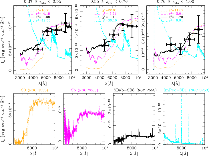
Figure 10.— Illustration of the SED fitting technique. In the bottom row we plot the rest-frame spectra (UV to near-IR) of four galaxies which are representative of the whole range of galaxy SEDs, from the early types (to the left) to the late and star-bursting types (to the right). The flux normalization is arbitrary. In the top panels the filled dots with error bars display the flux density in the four SDSS bands (observed frame) for the three $z_{abs}$ bins (low is to the left and high to the right). The horizontal error bars span the filter band-width. The lines represent the best-fit renormalized spectra computed by convolving the redshifted templates of the bottom row with the redshift distribution of the absorbers (see text for details). The line styles and colors are the same as in the bottom panels. The $\chi^{2}$ of each model is reported as well. Note how much better the intermediate type templates (NGC 7552 in particular) match the observational data at all redshifts.

Table 3Integral photometry and colors

$W_{0}(2796)$ bin	Radial range	Integral flux (mag)				Color (mag)
		g	r	i	z	g-r	r-i	i-z
$0.37\leq z_{abs}<0.55$
Low-$W_{0}$	10– 50 kpc	$23.50^{+0.49}_{-0.34}$	$22.00^{+0.21}_{-0.17}$	$21.40^{+0.21}_{-0.17}$	$20.82^{+0.29}_{-0.23}$	$1.50\pm 0.34$	$0.60\pm 0.12$	$0.57\pm 0.23$
	50–100 kpc	$23.88^{+\inf}_{-0.77}$	$21.81^{+0.30}_{-0.24}$	$21.12^{+0.29}_{-0.23}$	$20.52^{+0.53}_{-0.36}$	$2.08\pm 0.99$	$0.69\pm 0.18$	$0.60\pm 0.39$
	10–100 kpc	$22.92^{+0.88}_{-0.48}$	$21.14^{+0.21}_{-0.18}$	$20.50^{+0.22}_{-0.18}$	$19.91^{+0.36}_{-0.27}$	$1.78\pm 0.53$	$0.65\pm 0.13$	$0.59\pm 0.29$
Intermediate-$W_{0}$	10– 50 kpc	$22.95^{+0.28}_{-0.22}$	$22.18^{+0.24}_{-0.19}$	$21.88^{+0.30}_{-0.24}$	$22.02^{+1.26}_{-0.57}$	$0.76\pm 0.22$	$0.31\pm 0.19$	$-0.14\pm 0.67$
	50–100 kpc	$24.38^{+\inf}_{-1.04}$	$22.71^{+0.73}_{-0.43}$	$22.27^{+0.96}_{-0.50}$	$21.25^{+1.15}_{-0.55}$	$1.67\pm 1.60$	$0.44\pm 0.48$	$1.02\pm 0.78$
	10–100 kpc	$22.69^{+0.64}_{-0.40}$	$21.66^{+0.29}_{-0.23}$	$21.30^{+0.41}_{-0.30}$	$20.81^{+0.95}_{-0.50}$	$1.03\pm 0.44$	$0.36\pm 0.26$	$0.49\pm 0.61$
High-$W_{0}$	10– 50 kpc	$22.54^{+0.19}_{-0.16}$	$21.58^{+0.14}_{-0.13}$	$21.09^{+0.14}_{-0.13}$	$20.59^{+0.22}_{-0.18}$	$0.97\pm 0.14$	$0.48\pm 0.08$	$0.50\pm 0.18$
	50–100 kpc	$23.34^{+1.08}_{-0.53}$	$22.13^{+0.41}_{-0.30}$	$21.85^{+0.54}_{-0.36}$	$21.35^{+1.24}_{-0.56}$	$1.21\pm 0.59$	$0.28\pm 0.31$	$0.50\pm 0.70$
	10–100 kpc	$22.12^{+0.35}_{-0.26}$	$21.07^{+0.19}_{-0.16}$	$20.65^{+0.21}_{-0.17}$	$20.15^{+0.39}_{-0.29}$	$1.05\pm 0.25$	$0.41\pm 0.14$	$0.50\pm 0.31$
All	10– 50 kpc	$22.89^{+0.15}_{-0.13}$	$21.86^{+0.10}_{-0.09}$	$21.39^{+0.11}_{-0.10}$	$20.97^{+0.18}_{-0.15}$	$1.03\pm 0.11$	$0.47\pm 0.07$	$0.42\pm 0.15$
	50–100 kpc	$23.75^{+0.82}_{-0.46}$	$22.16^{+0.22}_{-0.18}$	$21.67^{+0.25}_{-0.20}$	$21.00^{+0.40}_{-0.29}$	$1.59\pm 0.50$	$0.49\pm 0.16$	$0.67\pm 0.32$
	10–100 kpc	$22.49^{+0.27}_{-0.21}$	$21.25^{+0.12}_{-0.11}$	$20.77^{+0.14}_{-0.12}$	$20.23^{+0.24}_{-0.20}$	$1.24\pm 0.21$	$0.48\pm 0.09$	$0.54\pm 0.21$
$0.55\leq z_{abs}<0.76$
low-$W_{0}$	10– 50 kpc	$24.64^{+1.15}_{-0.54}$	$23.48^{+0.45}_{-0.32}$	$22.83^{+0.41}_{-0.30}$	$22.60^{+1.18}_{-0.55}$	$1.16\pm 0.60$	$0.65\pm 0.29$	$0.23\pm 0.70$
	50–100 kpc	$24.07^{+1.31}_{-0.58}$	$23.61^{+1.27}_{-0.57}$	$22.43^{+0.53}_{-0.35}$	$21.19^{+0.52}_{-0.35}$	$0.45\pm 0.80$	$1.18\pm 0.59$	$1.24\pm 0.51$
	10–100 kpc	$23.56^{+0.98}_{-0.51}$	$22.79^{+0.59}_{-0.38}$	$21.86^{+0.38}_{-0.28}$	$20.93^{+0.54}_{-0.36}$	$0.77\pm 0.59$	$0.93\pm 0.35$	$0.93\pm 0.47$
Intermediate-$W_{0}$	10– 50 kpc	$24.14^{+0.54}_{-0.36}$	$22.90^{+0.23}_{-0.19}$	$22.28^{+0.23}_{-0.19}$	$22.02^{+0.51}_{-0.35}$	$1.23\pm 0.38$	$0.62\pm 0.17$	$0.26\pm 0.39$
	50–100 kpc	$24.30^{+2.40}_{-0.69}$	$23.73^{+1.26}_{-0.57}$	$22.51^{+0.56}_{-0.37}$	$22.34^{+4.20}_{-0.74}$	$0.56\pm 1.01$	$1.22\pm 0.59$	$0.17\pm 1.09$
	10–100 kpc	$23.46^{+0.85}_{-0.47}$	$22.49^{+0.36}_{-0.27}$	$21.64^{+0.29}_{-0.23}$	$21.42^{+0.81}_{-0.46}$	$0.97\pm 0.57$	$0.85\pm 0.25$	$0.22\pm 0.60$
High-$W_{0}$	10– 50 kpc	$23.35^{+0.21}_{-0.18}$	$22.33^{+0.12}_{-0.11}$	$21.81^{+0.13}_{-0.12}$	$21.74^{+0.37}_{-0.28}$	$1.02\pm 0.17$	$0.51\pm 0.10$	$0.07\pm 0.30$
	50–100 kpc	$23.78^{+0.67}_{-0.41}$	$22.71^{+0.35}_{-0.26}$	$22.08^{+0.35}_{-0.27}$	$22.39^{+\inf}_{-0.79}$	$1.08\pm 0.47$	$0.63\pm 0.26$	$-0.31\pm 1.11$
	10–100 kpc	$22.79^{+0.31}_{-0.24}$	$21.75^{+0.17}_{-0.15}$	$21.19^{+0.18}_{-0.16}$	$21.27^{+0.73}_{-0.43}$	$1.05\pm 0.25$	$0.56\pm 0.14$	$-0.08\pm 0.52$
All	10– 50 kpc	$23.88^{+0.21}_{-0.18}$	$22.79^{+0.11}_{-0.10}$	$22.22^{+0.12}_{-0.10}$	$22.06^{+0.28}_{-0.22}$	$1.10\pm 0.17$	$0.57\pm 0.09$	$0.16\pm 0.24$
	50–100 kpc	$24.01^{+0.50}_{-0.34}$	$23.21^{+0.32}_{-0.25}$	$22.31^{+0.24}_{-0.19}$	$21.81^{+0.50}_{-0.34}$	$0.80\pm 0.39$	$0.90\pm 0.22$	$0.50\pm 0.41$
	10–100 kpc	$23.19^{+0.29}_{-0.23}$	$22.23^{+0.16}_{-0.14}$	$21.51^{+0.14}_{-0.13}$	$21.17^{+0.33}_{-0.25}$	$0.97\pm 0.23$	$0.72\pm 0.12$	$0.34\pm 0.29$
$0.76\leq z_{abs}<1.00$
low-$W_{0}$	10– 50 kpc	$24.26^{+0.43}_{-0.31}$	$24.53^{+1.10}_{-0.54}$	$23.23^{+0.41}_{-0.30}$	$22.65^{+0.77}_{-0.45}$	$-0.27\pm 0.66$	$1.30\pm 0.57$	$0.58\pm 0.56$
	50–100 kpc	$24.87^{+\inf}_{-0.78}$	$24.95^{+\inf}_{-1.03}$	$23.03^{+0.77}_{-0.44}$	$23.11^{+\inf}_{-1.02}$	$-0.08\pm 1.80$	$1.91\pm 1.47$	$-0.08\pm 1.63$
	10–100 kpc	$23.77^{+0.80}_{-0.45}$	$23.97^{+2.30}_{-0.69}$	$22.38^{+0.50}_{-0.34}$	$22.10^{+1.76}_{-0.64}$	$-0.20\pm 0.95$	$1.59\pm 0.78$	$0.27\pm 0.85$
Intermediate-$W_{0}$	10– 50 kpc	$24.52^{+0.50}_{-0.34}$	$23.82^{+0.33}_{-0.25}$	$23.59^{+0.51}_{-0.35}$	$22.65^{+0.67}_{-0.41}$	$0.70\pm 0.39$	$0.23\pm 0.37$	$0.94\pm 0.58$
	50–100 kpc	$...^{+...}_{-...}$	$24.13^{+1.27}_{-0.57}$	$23.55^{+1.30}_{-0.57}$	$21.94^{+0.78}_{-0.45}$	$...\pm...$	$0.58\pm 0.73$	$1.61\pm 0.85$
	10–100 kpc	$24.57^{+9.19}_{-0.75}$	$23.21^{+0.53}_{-0.35}$	$22.82^{+0.67}_{-0.41}$	$21.48^{+0.61}_{-0.39}$	$1.37\pm 1.01$	$0.39\pm 0.44$	$1.33\pm 0.62$
High-$W_{0}$	10– 50 kpc	$23.90^{+0.25}_{-0.20}$	$23.74^{+0.29}_{-0.23}$	$22.75^{+0.21}_{-0.17}$	$22.52^{+0.58}_{-0.38}$	$0.16\pm 0.27$	$0.99\pm 0.24$	$0.23\pm 0.45$
	50–100 kpc	$24.24^{+0.80}_{-0.46}$	$24.47^{+2.39}_{-0.69}$	$23.87^{+2.71}_{-0.71}$	$23.43^{+\inf}_{-1.14}$	$-0.23\pm 0.90$	$0.59\pm 0.99$	$0.44\pm 2.17$
	10–100 kpc	$23.30^{+0.38}_{-0.28}$	$23.29^{+0.51}_{-0.35}$	$22.42^{+0.41}_{-0.30}$	$22.13^{+1.46}_{-0.60}$	$0.01\pm 0.40$	$0.87\pm 0.37$	$0.29\pm 0.85$
All	10– 50 kpc	$24.19^{+0.19}_{-0.16}$	$23.94^{+0.22}_{-0.18}$	$23.12^{+0.17}_{-0.15}$	$22.59^{+0.33}_{-0.25}$	$0.24\pm 0.21$	$0.82\pm 0.18$	$0.53\pm 0.29$
	50–100 kpc	$24.96^{+1.04}_{-0.52}$	$24.39^{+0.77}_{-0.45}$	$23.44^{+0.52}_{-0.35}$	$22.60^{+0.83}_{-0.47}$	$0.57\pm 0.71$	$0.94\pm 0.48$	$0.84\pm 0.65$
	10–100 kpc	$23.75^{+0.35}_{-0.26}$	$23.39^{+0.33}_{-0.25}$	$22.52^{+0.26}_{-0.21}$	$21.84^{+0.46}_{-0.32}$	$0.36\pm 0.33$	$0.87\pm 0.25$	$0.68\pm 0.40$

We illustrate the main results of this analysis in Figure 10. Here we consider the three $z_{abs}$ subsamples. In the three panels in the top row the observed flux densities, derived from the integrated magnitudes between 10 and 100 kpc (see table 3) in the three $z_{abs}$ bins, are reported as the orange filled dots with error-bars (the horizontal error-bars represent the effective width of each passband). For the sake of illustration, we now consider only four SED templates that are representive of the whole range of galaxies. Their rest-frame spectra are shown in the four panels of the bottom row. From left to the right, we consider:
a) a typical early-type spectrum (from the S0 galaxy NGC 1553), characterized by a very suppressed UV flux, strong 4000 Å  break and metal lines, and flat shape at $\lambda>6000$ Å.
b) the spectrum of an intermediate spiral galaxy (from the Sb galaxy NGC 7083), which is characterized by stronger UV flux, a weaker 4000 Å  break, weak emission lines, and very moderate blue slope in the continuum at $\lambda>6000$ Å.
c) an early type spiral (NGC7552, SBab) which is undergoing a starburst, partially attenuated by dust (StarBurst class 6 in the atlas of Calzetti et al., 1994); the unattenuated blue continuum longward of the 4000 Å  break and the strong emission lines coming from the star-burst coexist with a strong 4000 Å  break and strongly suppressed UV flux, typical of the unextincted old stellar population.
d) Finally, the fourth panel shows the spectrum of an unextincted starburst galaxy (NGC 5253, starburst class 1 in the atlas of Calzetti et al., 1994), which is characterized by blue optical continuum, strong emission lines, and highly enhanced UV flux.

These four spectra are redshifted and convolved with the distribution of $z_{abs}$ and normalized to the observed data points as explained above. The results are reported in the three top panels of Figure 10, where different line styles and colors code the four original spectra. We also report the $\chi^{2}$ relative to each model. It is apparent that the two extreme templates (passive early type and pure star burst) completely fail to reproduce the observations at any redshift. Good fits are obtained only with the intermediate types, with the best results coming from the intermediate spiral with partially obscured starburst. This latter young component appears to be particularly required in order to reproduce the observed “jump” due to the 4000 Å  break, which in addition, is required to be weaker than in a normal Sb galaxy. A striking result from Figure 10 is also the fact that the same template is the best fit to the observed fluxes at all redshifts. In other words, we do not observe any significant evolution in the average SED of galaxies associated with MgII absorbers from $z=0.4$ to $z=1$, which validates our assumption of negligible redshift evolution.

From FIgure 10 we also note that the SDSS bands mainly constrain the rest-frame $u$ and $g$ flux. In the highest redshift bin the situation is even more extreme, as the $g$-, $r$-, and $i$-bands sample the flux blue-wards of the 4000 Å  break, while the $z$-band is not very sensitive; this results in a very poor constraint to the global properties of the stellar populations, and in an over-sensitivity to the effects of dust attenuation in the rest-frame UV at $z_{abs}\gtrsim 0.6$.

5.1. SED fitting analysis

We now extend our analysis, using the complete library of the 39 UV-optical spectra selected as reported above, to assess the previous result statistically, and in terms of rest-frame colors and luminosities. All templates are classified by morphology (according to NED) and their rest-frame colors, $u-g$, $g-r$, $r-i$, are synthesized from the spectrum. The distribution of the templates in this 3-dimensional color space is plotted in Figures 11 and 12, for different absorber subsamples, respectively. In each of these figures, the morphological type of the SED template, from Elliptical-S0 to Irregular/Blue Compact Dwarf galaxies, is coded according to the symbol shape (from circles to triangles) and color, whereas the size scales inversely to the $\chi^{2}$, as indicated in the legend. The best-fit model is identified by the cross-hairs; all models that result in $\chi^{2}<6$ (or a $\chi^{2}$ per degree of freedom less than 2) are identified by the open symbols, while other models are represented by the filled ones.

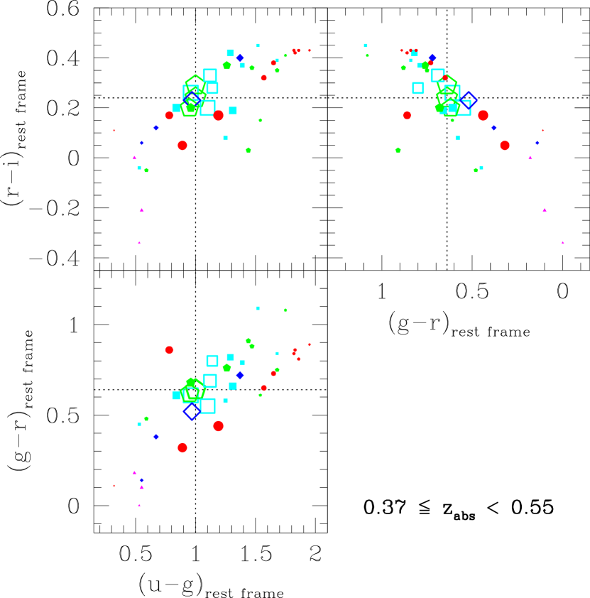
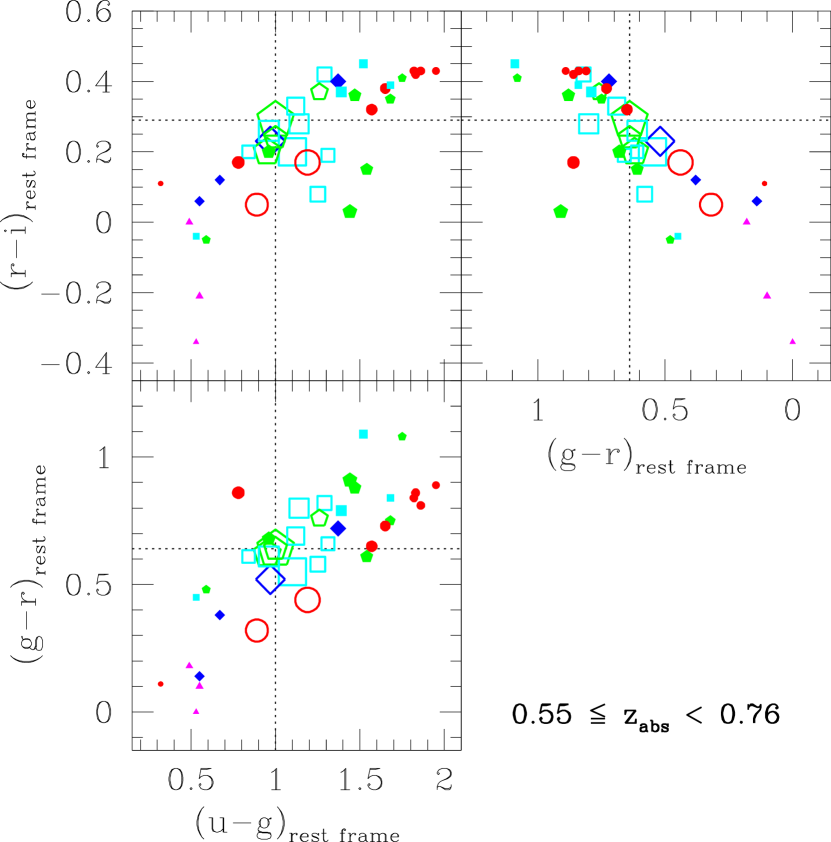
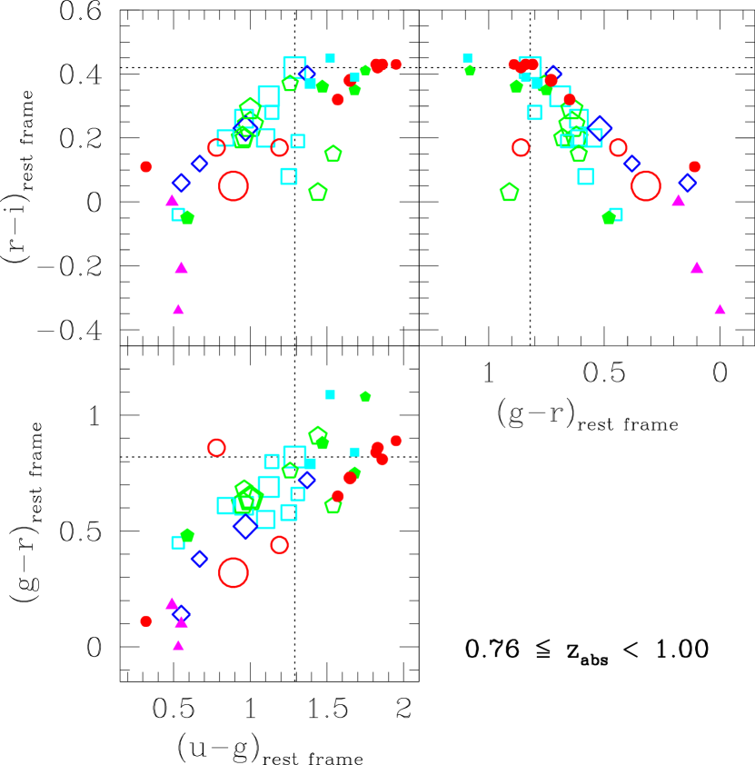
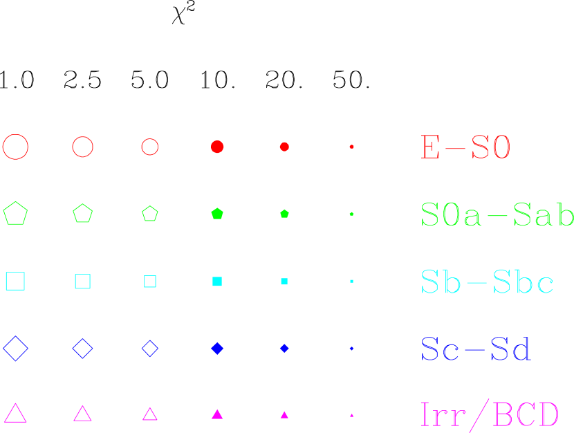
Figure 11.— “Goodness of fit” distribution in the rest-frame color space for the three $z_{abs}$ samples. Each point represents a template galaxy spectrum (taken from Calzetti et al., 1994; McQuade et al., 1995; Storchi-Bergmann et al., 1995), whose corresponding morphology is coded by its shape and color, as indicated in the legend. The size of the symbol is inversely related to the $\chi^{2}$ of the template, as from legend. The best fitting template is marked by the cross-hairs, while all templates yielding $\chi^{2}<6$ (our confidence limit, see in the text for details) are coded with open symbols. All other templates are shown as filled symbols.

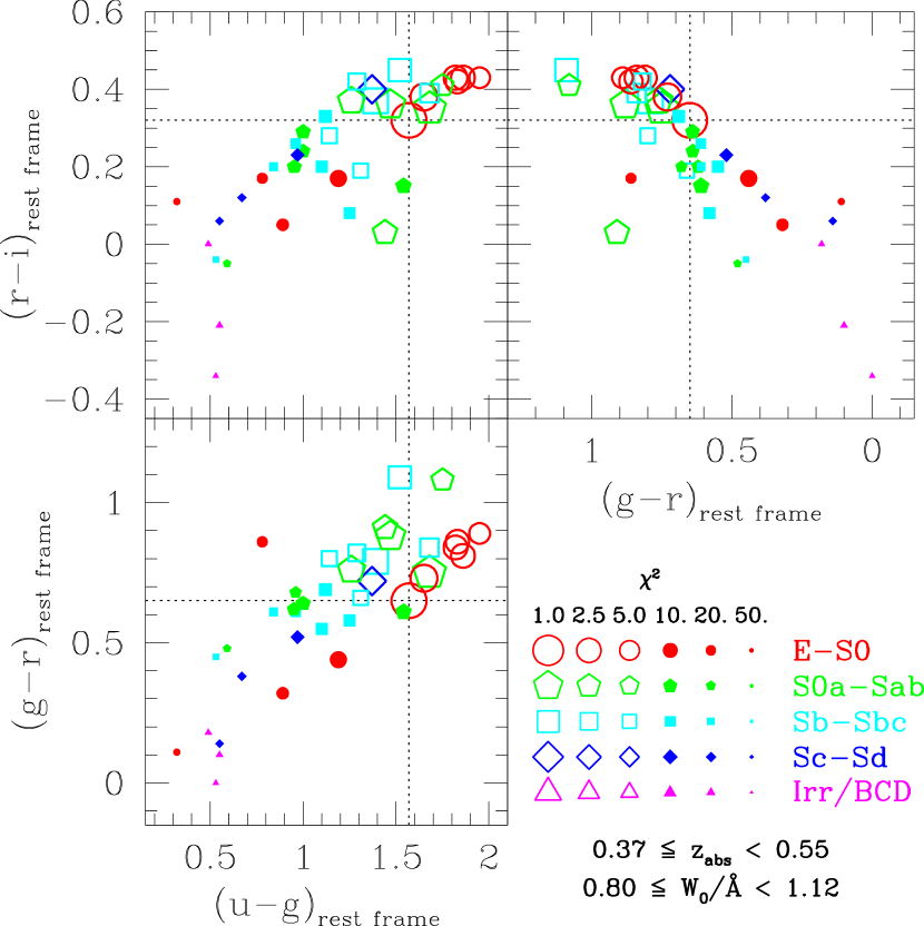
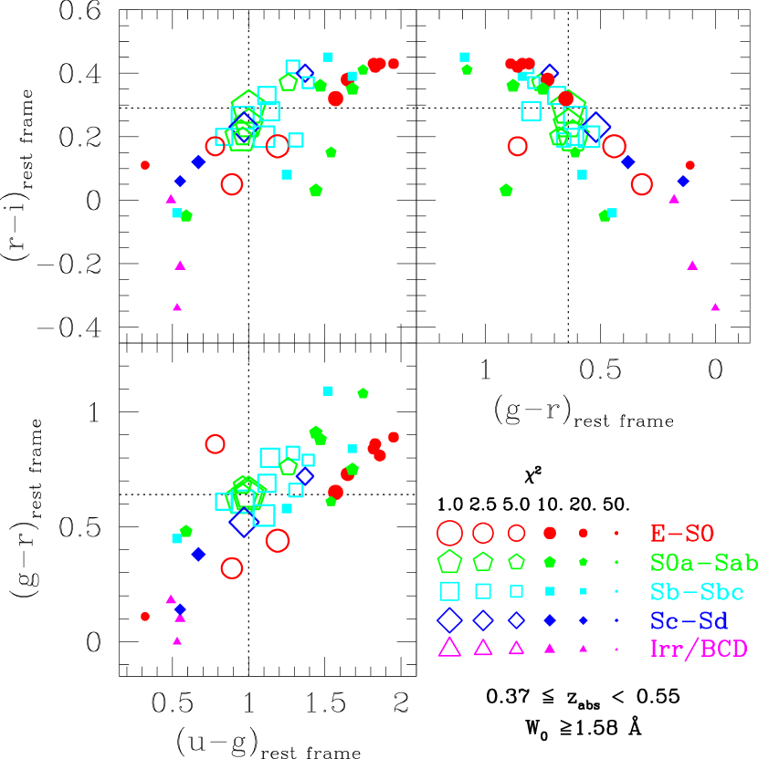
Figure 12.— “Goodness of fit” distribution in the rest-frame color space for the two extreme bin of EW at low $z_{abs}$: the results for the ‘low-$W_{0}$ systems are shown in the left panel, high-$W_{0}$ systems are shown on the right. Plotted quantities are the same as Figure 11.

We immediately observe that the rest-frame $u-g$ color, and, to a lesser extent, the $g-r$ are well constrained by our observations, and indicate that the average SED of the absorbing galaxies is consistent with intermediate-type spiral galaxies (Sab to Sbc) of the local Universe at all studied redshifts (Figure 11). We consider the colors of the best-fit model as best estimates of the rest-frame colors and $\chi^{2}=6$ as a confidence limit, and report these values in columns 2, 3, and 4 of Table 4. We conclude that in the entire redshift range 0.36$<z<$1.0 the average SED of the absorbing galaxies is characterized by rest-frame colors $u-g=1.1\pm 0.2$, $g-r=0.8\pm 0.2$, and $r-i=0.3\pm 0.1$.

Table 4Rest-frame colors and luminosities

$W_{0}(2796)$ bin	$u-g$	$g-r$	$r-i$	$u$	$g$	$r$	$i$	$\delta M$
	mag	mag	mag	mag	mag	mag	mag	mag
(1)	(2)	(3)	(4)	(5)	(6)	(7)	(8)	(9)
$0.37\leq z_{abs}<0.55$
All ($<100$ kpc)	$1.14^{+.25}_{-.19}$	$0.80^{+.02}_{-.36}$	$0.28^{+.14}_{-.11}$	$-19.57$	$-20.65$	$-21.45$	$-21.73$	$0.11$
All ($<50$ kpc)	$1.00^{+.14}_{-.05}$	$0.64^{+.16}_{-.12}$	$0.24^{+.09}_{-.04}$	$-19.02$	$-20.02$	$-20.66$	$-20.90$	$0.09$
low-$W_{0}$ ($<100$ kpc)	$1.57^{+.38}_{-.43}$	$0.65^{+.44}_{-.00}$	$0.32^{+.13}_{-.29}$	$-19.37$	$-20.94$	$-21.59$	$-21.91$	$0.17$
high-$W_{0}$ ($<100$ kpc)	$1.00^{+.39}_{-.22}$	$0.64^{+.22}_{-.32}$	$0.29^{+.13}_{-.24}$	$-19.71$	$-20.71$	$-21.35$	$-21.64$	$0.17$
$0.55\leq z_{abs}<0.76$
All ($<100$ kpc)	$1.00^{+.31}_{-.16}$	$0.64^{+.18}_{-.32}$	$0.29^{+.13}_{-.14}$	$-19.92$	$-20.92$	$-21.56$	$-21.85$	$0.12$
$0.76\leq z_{abs}<1.00$
All ($<100$ kpc)	$1.29^{+.25}_{-.29}$	$0.82^{+.09}_{-.68}$	$0.42^{+.00}_{-.46}$	$-19.90$	$-21.19$	$-22.01$	$-22.43$	$0.20$

By applying the same kind of analysis to the two subsamples of low-$W_{0}$ (Figure 12 left panel) and high-$W_{0}$ systems (Figure 12 right panel) at low redshift, we observe significant differences between the two classes; i.e., the colors of low-$W_{0}$ systems are best fitted by the template of an elliptical galaxy and the high-$W_{0}$ systems appear to be significantly bluer. This is shown quantitatively in Table 4 where we can see strong differences in $u-g$ between the two subsamples. At low redshift high-$W_{0}$ systems are about 0.6 mag bluer than low-$W_{0}$ ones. At higher redshift the signal is too weak to perform a similar analysis.

The difference between the SEDs of low- and high-$W_{0}$ systems is particularly well illustrated in Figure 13, where we plot the best fitting SEDs for the three bins of $W_{0}$ at low redshift. The top half of each panel reproduces the observed photometric data points overlaid on the convolved and normalized template spectrum, while the bottom half displays the original template spectrum. It is apparent that the weakest systems are best reproduced by a red passive template, while at $W_{0}\gtrsim 1.1$Å the SED closely resembles those of local actively star-forming galaxies.

From the fitting of the SED we also derive the normalization factor, which enables us to compute rest-frame luminosities in different bands. As mentioned above, the best constraints are obtained for the rest-frame $u-$ and $g-$ band fluxes, which correspond to the central and most sensitive $r$- and $i$-band in the observed frame. The uncertainty in these fluxes is driven mainly by the photometric errors. On the other hand, the rest-frame $r-$ and $i-$ band fluxes are extrapolated with the aid of the template SED, and therefore are subject to the additional uncertainty of the choice of the SED template. This is clearly the major source of error in the reddest rest-frame bands at high redshift. In Table 4, we report the rest-frame absolute magnitudes in $u$, $g$, $r$, and $i$ in columns 5, 6, 7, and 8, respectively, for different absorber subsamples. The uncertainty in the normalization factor, which is given purely by the photometric error, is given in column 9. This is computed as the variation of the normalization factor which is required to increase the value of $\chi^{2}$ by 1 with respect to the minimum while adopting the best fit template. All the following considerations are made using photometric quantities integrated between 10 and 100 kpc. Looking at the rest-frame luminosity in $u$ and $g$ as a function of redshift we note a significant trend with higher redshift systems having higher luminosity; the increase is roughly 30 to 50% from $z\sim 0.4$ to $z\sim 0.9$. It must be noted that such a luminosity evolution has a negligible impact on our interpretation of colors within each $z_{abs}$ bin; in fact, taking luminosity evolution into account changes the observed-frame colors synthesized from the model SEDs by 0.02 mag at most for intermediate galaxy spectral types.

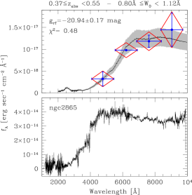
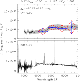
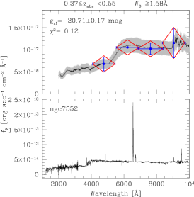
Figure 13.— The best fitting templates for the three $W_{0}$ bins at low redshift, from the weakest systems (to the left) to the strongest ones (to the right). In each graph, the rest-frame template spectrum is plotted in the bottom panel, with some arbitrary intensity normalization, and identified by the NGC name of the galaxy. The top panels show the measured photometric points (red diamonds, whose vertical extent indicates the absolute photometric error in each band individually) overlaid on the convolved and re-normalized template spectrum (see text for details). The blue points with error bars show the error relative to the $r$-band data points. The shaded area is the 1-$\sigma$ confidence range allowed for the normalization. The best fitting rest-frame $g$ magnitude is also reported, along with the (non-reduced) $\chi^{2}$.

It is worth noting here that luminosities and colors are scale-dependent. This effect is illustrated in Table 4 where we report the colors and luminosities for the low-$z_{abs}$ sample measured between 10 and 50 kpc. With respect to the total quantities the rest-frame luminosities are lowered by 0.45 ($u$-band) to 0.83 mag ($i$-band), while the colors are systematically bluer. This color gradient is primarily a consequence of the fact that strong systems, which are also bluer, are more concentrated and dominate the total light in the inner tens of kpc.

5.2. The SED and luminosity of MgII absorbing galaxies in context

At the beginning of this section we presented an interpretation of the colors of the absorbing galaxies in terms of local galaxy spectral templates. We showed that the average SED is typical of intermediate type galaxies, with both old stellar populations and a starburst component. This mix varies going from low- to high-$W_{0}$ absorbers, with the latter having an enhanced starburst component. It is interesting to note that, in a different context, Kacprzak et al. (2006) have recently obtained a result that goes in this same direction, showing a positive correlation between $W_{0}$ and the ratio between the asymmetry parameter, $A$, and impact parameter for a sample of 24 intermediate redshift absorbing galaxies. By interpreting $A$ as an index of galaxy “activity”, the observed correlation is fully consistent with our finding that higher $W_{0}$ absorbers are associated with galaxies having a smaller impact parameter and a more “active” SED (in the sense of star formation). The correlation between star formation and EW is further supported by the observation, reported by Nestor et al. (2005), that strong systems occur with a relatively higher frequency at high redshift $\gtrsim 1$, thus paralleling the evolution of the cosmic star formation rate.

No evidence is found for significant redshift evolution of the average SED. This is an argument in favor of the thesis that MgII absorption systems trace a well defined evolutionary phase of galaxies, rather than just a particular class of halos or galaxies in a fixed mass range.

In order to characterize this evolutionary phase in the cosmological context, we compare the average colors and luminosities of the absorbing galaxies with a well-understood sample of $I+B$-band selected galaxies from the FORS Deep Field survey (hereafter FDF, Heidt et al., 2003). In addition to multi-band photometry from the $U$ to the $K_{S}$-band, the FDF catalogs provide the photometric redshift of each galaxy and the best fitting SED template (see Bender et al., 2001). These can then be used to derive the rest-frame photometric properties of the galaxy, and to convert the observed magnitudes into the SDSS photometric system. We select all galaxies with absolute rest-frame $i$-band magnitudes brighter than $-17.0$, and split the sample into the same three redshift bins adopted for the absorbers.

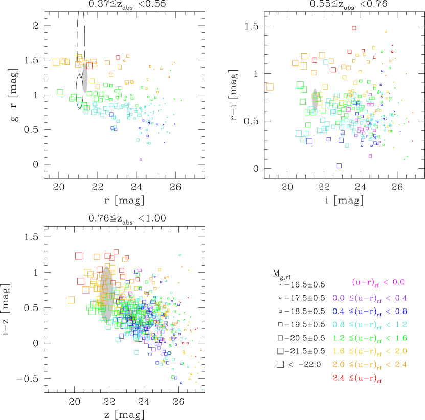
Figure 14.— The observed frame color-magnitude diagram (CMD) of galaxies selected from the FORS Deep Field (FDF), compared to our absorbers stack photometry in the three redshift bins. Points are FDF galaxies coded to indicate their rest-frame absolute $g$-band magnitude (size) and rest-frame $u-r$ color (color), as shown in the legend. The shaded ellipse is the 1-$\sigma$ confidence interval for color/magnitude of our stack photometry for the “All-” EW sample. In the low-$z_{abs}$ panel (upper left) we also display the fiducial estimates for the low- and high-$W_{0}$ absorber sub-samples with the dashed and solid ellipses, respectively.

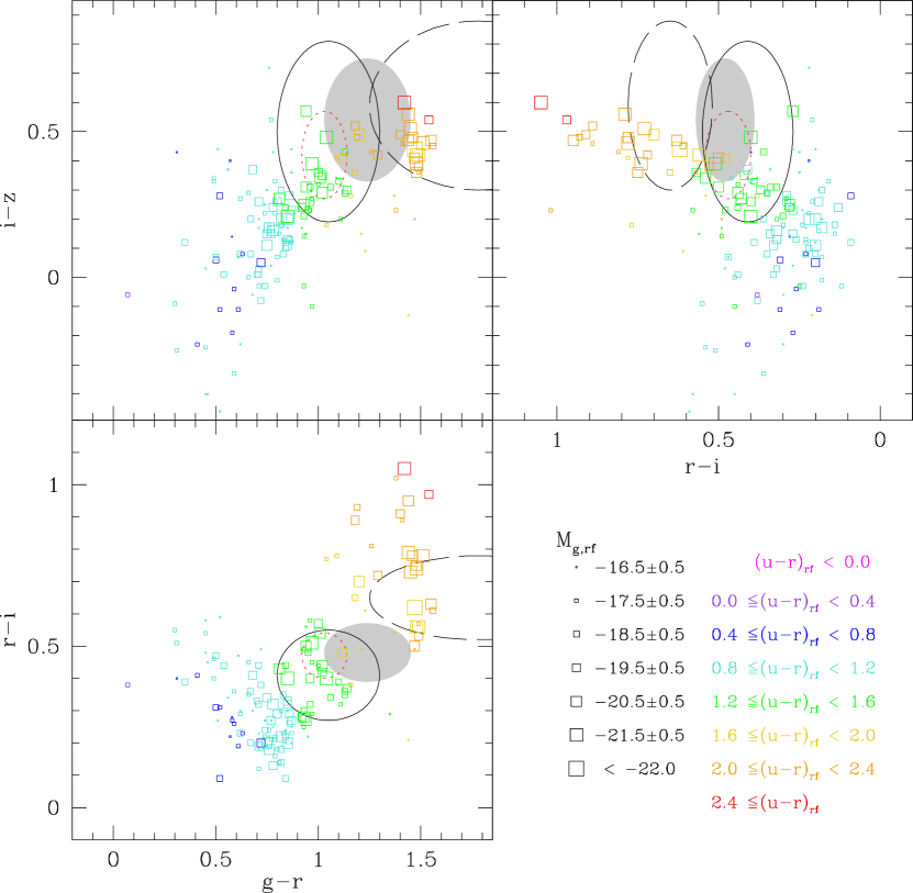
Figure 15.— The three projections of FDF galaxies in the observed frame $(g-r)$-$(r-i)$-$(i-z)$ observed color space, compared to our absorbers stack photometry in the low-$z_{abs}$ bin ($0.37\leq z_{abs}<0.55$). As in Figure 14, points are FDF galaxies coded to indicate their rest-frame absolute $g$-band magnitude (size) and rest-frame $u-r$ color (color), as shown in the legend. The shaded ellipse is the 1-$\sigma$ confidence interval for colors from our stack photometry for the “All” EW sample. High- and low-$W_{0}$ absorber sub-samples are shown with the solid and dashed ellipses, respectively. The red dotted ellipse is used to display the colors in the limited range 10-50 kpc.

Figure 14 shows the observed-frame color-magnitude diagram (CMD) of the FDF galaxies in the three redshift bins. Observed-frame bands and colors for different redshifts are chosen so as to correspond to similar rest-frame spectral regions, namely, the magnitude on the x-axis samples the flux at $\sim 4500$Å, while the color on the y-axis roughly corresponds to rest-frame $u-g$ in all three panels. The size of the square is indicative of the absolute $g$-band luminosity of each FDF galaxy (as shown in the figure legend), while the color of the symbol codes the rest-frame $u-r$, which is particularly suited to separate late- from early-type galaxies (e.g. Baldry et al., 2004). The photometric measurements relative to our absorbers, including all $W_{0}$, are indicated by the grey shaded ellipses in each panel, with the shaded area representing the 1-$\sigma$ confidence limits. For the low-$z_{abs}$ bin (upper left panel) we also overplot the two ellipses relative to the high-$W_{0}$ systems (solid line) and the low-$W_{0}$ ones (dashed line). Note that we always refer to photometric quantities within the 100 kpc aperture, unless specified otherwise.

It appears that the average colors of the absorbing galaxies are intermediate between the very red ones ($(u-r)_{rf}\geq 1.6$) of passive galaxies on the red sequence (the ridge of yellow-red points visible in the two top panels of Figure 14) and the bluer colors, that characterize star forming spirals of intermediate luminosity. This, again, is seen at all redshifts. We can thus conclude that the average colors of the absorbing galaxies are intermediate not only in absolute sense (as we already saw from the fit of local SED templates), but also relative to the galaxies of similar luminosity at the same redshift. Figure 14 also supports the idea that MgII absorbers reside in halos hosting a $L\lesssim L^{\star}$ galaxy. In fact, if the total observed luminosity arose from a large number of low-luminosity galaxies, then we would expect much bluer colors than observed. Conversely, we note that the estimated absolute magnitude of the absorbing galaxies ($M_{i,rf}\sim-21.7$) is perfectly consistent with those of galaxies sharing the same region of the color-magnitude diagram.

Figure 14, and the low-$z_{abs}$ panel in particular, at first glance suggests that the absorbing galaxies could be those rare galaxies that populate the so-called “green valley” between the red sequence of passive galaxies and the blue sequence of the star-forming ones. In turn, this would imply that the galaxies linked to MgII absorbers are a kind of transition type that live in this phase for a very limited amount of time (on the order of a few hundred Myr). Alternatively, the intermediate color of the total sample may result from a kind of “morphological mix” of passive and actively star-forming galaxies. At the beginning of this §5 we noted that high-$W_{0}$ absorbers are linked to bluer and more star-forming galaxies than the low-$W_{0}$ systems. In Figure 14 the location of two ellipses for the high- and low-$W_{0}$ systems actually show that a systematic change in galaxy properties occurs as a function of $W_{0}$: while high-$W_{0}$ systems occupy the locus of luminous star-forming spirals, the low-$W_{0}$ ones overlap with passive red-sequence objects. In order to investigate whether the two classes of absorbers reflect the color bimodality of the overall galaxy population we can use the three projections of the $(g-r)$-$(r-i)$-$(i-z)$ color space. Figure 15 shows these distributions for the FDF galaxies in the low $z_{abs}$ bin, with the same symbols and conventions used in Figure 14 and reported in the legend. As in Figure 14, the shaded ellipse represents the confidence region for the complete low-$z_{abs}$ sample, while the solid and dashed ellipses are the confidence contours for the high- and low-$W_{0}$ subsamples, respectively. In addition, we also report a red dotted ellipse to represent the colors of the total low-$z_{abs}$ sample, but within the smaller aperture $10<R<50$ kpc. The $(r-i)$-$(g-r)$ projection of the color space appears particularly suited to divide between red, passive galaxies and blue, active ones. The average colors of the total sample fall exactly in between the two clouds, but now stronger systems are clearly separated from the weaker ones: the stronger systems have colors typical of star-forming spirals, while the weaker ones overlap only with passive galaxies. It should be noted that intermediate-$W_{0}$ absorbers have the same colors as stronger ones, thus indicating that the transition between active and passive types must be quite sharp and occurs at $W_{0}\sim 1$Å. This result indicates that absorbing galaxies are likely to be representative of a large range of normal galaxies with $L\lesssim L^{\star}$, whose color bimodality is also reproduced. Also, absorbers weaker than $\sim 1$Å are most likely associated with galaxies that have already moved to a phase of passive evolution, while stronger systems mainly reside in halos where the primary galaxy is still blue and actively star-forming. It is interesting to note that the link between color bimodality and EW holds also when so-called weak systems ($W_{0}<0.3$Å) are considered. Using 7 absorbers with WFPC2/HST imaging and spectroscopic spatial coverage Churchill et al. (2006) have recently shown that passive galaxies are also associated with such weak absorbers. Moreover, the clustering analysis conducted by Bouché et al. (2006) shows a similar tendency, i.e., weaker systems appear to be more clustered than stronger ones, which suggests that they are related to redder galaxies. However, while the trend is reproduced, the large dark matter halo masses inferred by their analysis for the low-EW systems differ from the $\lesssim L^{\star}$ luminosities found in the present study.

It should be noted that the average colors, and hence their interpretation in terms of spectral types, is dependent on the choice of the impact parameter limits. If one just considers the luminosity-weighted average color of absorbing galaxies within 50 kpc, instead of 100 kpc, bluer colors are obtained (as shown by the red ellipses in Figure 15, leading to the wrong conclusion that passive galaxies are much less abundant among the absorbers. Our extensive photometry represents a clear advantage in this sense, with respect to most of the previous spectro-photometric surveys that could cover only a limited range of impact parameters.

Finally, we have also observed a trend of increasing rest-frame luminosity with redshift (30 to 50% more luminous from $z\sim 0.4$ to 0.9). If we interpret the presence of MgII absorbers as indicative of a given evolutionary phase for a galaxy, this luminosity evolution can be seen as another phenomenon of downsizing, i.e., the occurrence of a given evolutionary phase is delayed in smaller galaxies.

6. Interpretation

In this section we attempt to interpret the observational results reported in this paper. We briefly discuss possible scenarios that may reproduce the spatial and photometric measurements presented above, encouraging detailed modeling in these directions.

In §4.2 we presented measurements of a spatial cross-correlation between MgII absorption and light, i.e., galaxies, and we have shown that such a quantity is related to a light weighted distribution of impact parameters. As explained above such observational results provide us with robust statistical constraints as they do not make use of any assumption about the nature, impact parameter and number of galaxies responsible for the absorption. Moreover, the large number of absorption systems analyzed (about 600 to 1250 in each redshift bin) allows us to measure the gas-light correlation up to about 200 kpc. It is important to note that the effects of galaxy clustering becomes increasingly important as we consider larger scales. The gas detected in absorption can be “related” to a given galaxy which can be closely surrounded by a number of neighbors. As recently shown by Churchill et al. (2005b) this has led to several misidentifications in the past.

Clustering effects are inherent to any statistical spatial studies and must be taken into account for interpreting results. Over the last few years, galaxy-galaxy lensing studies have illustrated this fact. This weak lensing technique provides us with a cross-correlation between mass and light. Studies have shown that the galaxy masses inferred from this technique have a significant contribution from their environment (Mandelbaum et al., 2006). Similar effects are expected for gas-light cross-correlations.

As we showed in §4.2, the slope of the spatial cross-correlation between gas and light strongly depends on the strength of the MgII absorbers. This change of slope can be due either to a clustering of the gas around galaxies being a function of $W_{0}$ or to a change in the galactic environment. Detailed modeling using, for example, the halo-model approach will be required to accurately interpret these results.

Regarding the photometric properties of the light found in the vicinity of MgII absorbers, we have shown that stronger absorbers are related to bluer galaxies. We have found that systems with $W_{0}\gtrsim 1$Å  have colors matching those of star-forming galaxies with $L\lesssim L^{\star}$. Similar results based on different techniques were reported in previous studies (e.g. Guillemin & Bergeron, 1997; Churchill et al., 1999). Bond et al. (2001) have also argued that the strong MgII systems can arise from the “blow out” of gaseous super-bubbles that are produced by supernovae explosions in starbursting regions. Based on kinematic studies of the MgII lines, Prochter et al. (2006) have recently brought new evidence that “the strong MgII phenomenon primarily arises from feedback processes in relatively low mass galactic halos related to star formation.” Our results on systems with $W_{0}\gtrsim 1$Å  indeed provide a statistically robust support to their conclusion, as far as the mass and the star-formation activity are concerned. We have shown that systems with $W_{0}\gtrsim 1.5$Å  are found to be in the direct vicinity of a galaxy: 50% of the associated light is within 25 kpc. Given typical super-wind expansion velocities of a few 100 km sec${}^{-1}\sim 1$ kpc Myr^-1 (Heckman et al., 2000), the MgII clouds have enough time to reach their observed location while the starburst is still active (assuming that the duration of the burst is of the order of 10 Myr). On the other hand we have shown that MgII systems weaker than $\sim 1.1$Å are found at larger impact parameter (50% of the galaxy light is beyond 50 kpc from the MgII system), and are predominantly associated with reddish and passive galaxies. A possible explanation may be that these weaker systems are also older, i.e., observed a longer period of time after their outflow from the parent galaxy. These MgII systems thus have had time to travel farther away from the galaxy, and in the meanwhile the burst has finished and the galaxy has turned into a passive red one. The interaction of the clouds with the intergalactic medium might explain the lower $W_{0}$; on long time-scales the MgII clouds can be eroded by hotter intergalactic gas and the multiple components that give rise to large $W_{0}$ are separated and diluted. Depending on the actual duration of the burst, we can estimate the time-scale to turn the SED of the high-$W_{0}$ absorbing galaxies into those of the weaker ones as something ranging from a few hundred Myr to 1 or 2 Gyr. Hence, the process of dilution of the MgII clouds has to become effective on the same time-scale, and the expansion speed at distances larger than 25 kpc must progressively slow down to roughly $30~{}\mathrm{kpc}/1~{}\mathrm{Gyr}\simeq 3~{}\mathrm{km}~{}\mathrm{sec}^{-1}$, in order to explain the broader distribution of impact parameters for weaker systems.

In contrast to outflow models, Mo & Miralda-Escude (1996) introduced a model in which metal absorption lines are related to gas infalling onto a galaxy which then triggers star formation. In such a scenario, weak systems are associated with galaxies that still have to accrete gas and trigger a (new) episode of star formation. In contrast, strong systems can be associated with the gas that is being accreted onto a galaxy and transformed into stars. The infall model therefore explains the anti-correlation between EW and impact parameter and also the correlation between blue colors and EW. In this model, weak absorbing galaxies must be interpreted as (the end of) a quiescent phase that precedes a new substantial burst of star formation, that will probably turn the galaxy back into a star-forming spiral. The minimum duration of this quiescent phase can be estimated to be 1-2 Gyr, i.e., the time to turn a galaxy red after a substantial episode of star formation, consistent with the observed mean SED of weak systems. However, such a kind of star formation history (SFH), with intense bursts interleaved with long quiescent periods, appears to be quite rare for $L\lesssim L^{\star}$ galaxies (corresponding to the integrated light found within 100 kpc of MgII absorbers). Such galaxies generally experience smooth continuous SFHs (Kauffmann et al., 2003). If such an interpretation can be confirmed quantitatively, it will show that the simple infall model does not contain the necessary mechanisms to reproduce the observed trends between the luminosity-weighted quantities and $W_{0}$.

6.1. Implications for DLA systems

Damped Lyman-$\alpha$ systems (DLAs) are believed to host most of the hydrogen in the Universe and provide the reservoir for star formation. As shown by Rao et al. (2006), strong MgII absorbers are often associated with DLAs and the correlation between the two increases as a function of $W_{0}(MgII)$. It is interesting to note that Rao et al. (2006) found that the mean $N_{HI}$ is roughly constant for MgII absorbers with $W_{0}\gtrsim 0.6$ Å  but dramatically decreases for weaker systems. This result is similar to the color change found between low- and high-$W_{0}$ systems: redder galaxies are expected to have converted a significant fraction of the available neutral hydrogen into stars. Moreover, while the colors of MgII absorbing galaxies appear to be similar in the range $W_{0}\gtrsim 1$Å, we detected a transition scale at $W_{0}\sim 1$Å, below which the colors become significantly redder. It would be of great interest to investigate whether other properties of metal absorbers or Lyman-$\alpha$ systems are seen to change around the scale of $W_{0}(MgII)\sim 0.6-1$Å. Understanding the origin of this value would give us important insights into the nature and properties of the gas in and around galaxies.

We can also note that, as the fraction of DLAs in MgII selected systems increases as a function of $W_{0}(MgII)$, our results suggest that stronger DLAs are expected to be associated with bluer galaxies, and more specifically, with more star forming galaxies.

7. Summary and conclusions

In this paper we present a statistical analysis that allows us to constrain the mean photometric properties of MgII absorbing galaxies and the impact parameter distribution of the gas. By stacking a large number of PSF-subtracted images of quasars with absorbers and comparing them with similar but non-absorbed quasars we isolate the excess light associated with MgII absorber systems and investigate its properties. Contrary to a number of previous studies which attempted to identify individual absorbing galaxies, our method measures a more general (and well defined) cross-correlation between gas and light, and does not use any assumption about the extent of the gas and/or a redshift interval within which the galaxy can be found. Moreover, it is directly applicable to large samples, and can probe large scales. In the present study we use a sample of about 2,800 quasar sightlines with one strong MgII absorber ($W_{0}(\lambda 2796)>0.8$ Å) and a control sample of more than 11,000 reference quasars extracted from SDSS DR4. The large number of systems allows us to study the properties of the absorbing galaxies as a function of redshift and rest equivalent width ($W_{0}$), thus partly compensating the loss of information inherent to any stacking procedure. Our results are as follows:

• We obtain significant detections of cross-correlations between MgII gas and light out to $\sim 200$ kpc scales. We show that the surface brightness (SB) distribution of such light is directly proportional to the impact parameter distribution of MgII systems around absorbing galaxies, weighted by galaxy luminosity.

• Over the range 20-100 kpc, the SB profiles or impact parameter distributions are well described by power laws with an index $\alpha$ that strongly depends on the rest equivalent width of the absorbers; $\alpha\simeq-1$ for low-EW systems ($0.8\mathrm{\AA}\leq W_{0}<1.12\mathrm{\AA}$), while $\alpha\simeq-2$ for high-EW systems ($W_{0}\geq 1.58\mathrm{\AA}$). More accurate fitting formulae are also provided in §4.3.

At low redshift, i.e. $0.37<z_{abs}\leq 0.55$, where the S/N is high enough, we find that

• the mean luminosity enclosed within $10$ kpc $<r<100$ kpc is $M_{g}=-20.65\pm 0.11$ for the global sample, which is $\sim 0.5~{}L_{g}^{\star}$ of the field luminosity function in the same redshift regime.

• The spectral energy distribution of stronger systems appears to be significantly bluer. MgII systems with $W_{0}>1$Å are, on average, characterized by an SED typical of star-forming/bursting galaxies, while the light of weaker systems is dominated by passive red galaxies (although they might not dominate the number counts).

Moreover, considering the entire redshift range $0.37<z<1.0$, we find:

• no detectable evolution with redshift of both spatial distribution and global average SED, which is always well fitted by intermediate type spirals. This suggests that MgII systems trace similar galaxies or a similar evolutionary phase of galaxies.

• The rest-frame optical luminosity increases by $\sim 50\%$ from $z\sim 0.4$ to $z\lesssim 1$. This phenomenon is reminiscent of the so-called downsizing which is observed in a number of indicators of galaxy activity.

We have discussed possible interpretations of these observations including inflowing/outflowing gas and clustering effects. While detailed modeling will be required to robustly test each model, we point out that a scenario in which metal-enriched gas outflows from star-forming/bursting galaxies is in qualitative agreement with several types of trends seen in the data.

The observational results presented in this paper, namely the cross-correlation between MgII gas and light and the mean colors of absorbing galaxies, provide robust statistical constraints of great interest for further modeling the gas distribution around galaxies. They will help produce a comprehensive and consistent picture of galaxy formation in both absorption and emission.

As a side-product of this study, we have shown that our stacking technique is able to detect the light of QSO hosts and their environment, thus opening new exciting perspectives for the study of the relationships between QSOs and galaxy formation.

Table 1Shape parameters of the absorbers’ SB profiles

$W_{0}(2796)$ bin	Powerlaw slope $\alpha$					First moment $R_{1}/\mathrm{kpc}$
	$g$	$r$	$i$	$z$	$<\alpha>$	$g$	$r$	$i$	$z$	$<R_{1}>$
(1)	(2)	(3)	(4)	(5)	(6)	(7)	(8)	(9)	(10)	(11)
$0.37\leq z_{abs}<0.55$
All	$-1.90^{+0.28}_{-0.37}$	$-1.62^{+0.19}_{-0.21}$	$-1.59^{+0.22}_{-0.23}$	$-1.36^{+0.33}_{-0.44}$	$-1.62\pm 0.13$	$39.2\pm 6.1$	$47.4\pm 2.4$	$47.8\pm 2.7$	$51.0\pm 3.8$	$47.6\pm 1.6$
low-$W_{0}$	$-2.27^{+0.84}_{-1.73}$	$-1.28^{+0.28}_{-0.32}$	$-0.93^{+0.30}_{-0.30}$	$-0.82^{+0.44}_{-0.48}$	$-1.08\pm 0.19$	$46.8\pm 11.8$	$54.8\pm 3.0$	$56.5\pm 2.8$	$56.2\pm 4.4$	$55.6\pm 1.8$
Intermediate-$W_{0}$	$-1.59^{+0.44}_{-0.56}$	$-1.36^{+0.36}_{-0.39}$	$-1.88^{+0.51}_{-0.72}$	$-0.31^{+0.49}_{-3.69}$	$-1.51\pm 0.27$	$33.9\pm 14.8$	$43.4\pm 6.4$	$43.5\pm 8.4$	$57.5\pm 9.1$	$45.7\pm 4.3$
High-$W_{0}$	$-2.14^{+0.44}_{-0.61}$	$-2.33^{+0.43}_{-0.55}$	$-2.25^{+0.40}_{-0.48}$	$-2.33^{+0.68}_{-1.30}$	$-2.25\pm 0.27$	$38.9\pm 7.5$	$43.8\pm 3.9$	$41.8\pm 4.7$	$42.8\pm 7.5$	$42.5\pm 2.6$
$0.55\leq z_{abs}<0.76$
All	$-1.32^{+0.30}_{-0.35}$	$-1.61^{+0.21}_{-0.22}$	$-1.26^{+0.16}_{-0.19}$	$-1.34^{+0.36}_{-0.44}$	$-1.38\pm 0.12$	$49.9\pm 4.6$	$47.2\pm 3.2$	$51.1\pm 2.5$	$55.0\pm 4.5$	$50.4\pm 1.7$
Low-$W_{0}$	$-0.71^{+0.16}_{-0.67}$	$-1.24^{+0.52}_{-0.63}$	$-0.86^{+0.41}_{-0.39}$	$-0.49^{+0.52}_{-0.66}$	$-0.82\pm 0.24$	$58.2\pm 9.0$	$50.7\pm 8.8$	$56.8\pm 5.0$	$69.0\pm 5.1$	$60.7\pm 3.1$
Intermediate-$W_{0}$	$-1.40^{+0.78}_{-1.45}$	$-2.46^{+0.51}_{-0.67}$	$-1.70^{+0.37}_{-0.45}$	$-2.07^{+0.79}_{-1.41}$	$-1.92\pm 0.31$	$50.9\pm 10.4$	$45.1\pm 7.2$	$51.2\pm 4.9$	$49.8\pm 11.7$	$49.5\pm 3.6$
High-$W_{0}$	$-1.60^{+0.33}_{-0.40}$	$-1.43^{+0.21}_{-0.22}$	$-1.31^{+0.26}_{-0.27}$	$-1.56^{+0.61}_{-0.94}$	$-1.43\pm 0.15$	$45.5\pm 5.8$	$46.7\pm 3.4$	$48.0\pm 3.5$	$40.7\pm 13.5$	$46.9\pm 2.2$
$0.76\leq z_{abs}<1.00$
All	$-1.92^{+0.30}_{-0.38}$	$-1.42^{+0.27}_{-0.30}$	$-1.42^{+0.27}_{-0.31}$	$-1.45^{+0.57}_{-0.80}$	$-1.55\pm 0.17$	$43.6\pm 6.6$	$44.8\pm 6.4$	$49.6\pm 4.3$	$53.3\pm 6.3$	$48.3\pm 2.8$
Low-$W_{0}$	$-1.82^{+0.64}_{-1.06}$	$-1.07^{+0.45}_{-1.38}$	$-0.65^{+0.35}_{-0.53}$	$-1.72^{+1.07}_{-2.28}$	$-0.96\pm 0.35$	$42.8\pm 12.7$	$42.6\pm 20.9$	$56.7\pm 5.5$	$46.9\pm 19.0$	$53.4\pm 4.8$
Intermediate-$W_{0}$	$-2.50^{+0.68}_{-1.15}$	$-1.42^{+0.34}_{-0.38}$	$-1.58^{+0.53}_{-0.72}$	$-1.23^{+0.93}_{-1.34}$	$-1.55\pm 0.29$	$33.0\pm 32.6$	$47.7\pm 8.2$	$50.9\pm 8.9$	$64.5\pm 5.8$	$56.7\pm 4.1$
High-$W_{0}$	$-1.63^{+0.33}_{-0.42}$	$-1.77^{+0.50}_{-0.63}$	$-2.03^{+0.43}_{-0.52}$	$-1.58^{+1.06}_{-2.42}$	$-1.78\pm 0.26$	$47.2\pm 6.4$	$41.2\pm 11.0$	$42.1\pm 8.3$	$39.5\pm 20.4$	$44.3\pm 4.5$

Appendix A On the origin of the signal in reference QSOs

In §4.1 we noted that the PSF subtraction leaves significant SB residues even in the sample of reference QSOs. In this appendix we further investigate the origin of this effect and demonstrate that this is not due to a failure of the PSF subtraction algorithm, rather to a genuine light excess found around QSOs with respect to the actual PSF. To do this, we stack images of reference QSOs only, without applying any geometrical transformation to the images (apart from centering). We consider as possible factors of mismatch with respect to the PSF:

• the redshift of the QSO. This is the case when the light excess is physically associated with the QSO, e.g. its host galaxy.

• the magnitude of the QSO. This is the case when either the excess is linked to intrinsic QSO properties, or when it arises from a failure in deblending faint sources.

• the color mismatch between the QSO and the star used to compute the PSF. In fact, redder point sources are expected to have a narrower PSF (see e.g. Fried, 1965).

We split the three-dimensional parameter space given by $z_{QSO}$, the QSO apparent magnitude in $i$-band $i_{QSO}$, and the color mismatch $\Delta(g-r)\equiv(g-r)_{star}-(g-r)_{QSO}$ into $3^{3}$ cells including roughly an equal number of reference QSOs ($\sim 400$). Each of these $3^{3}$ subsamples is then processed and stacked separately. We take the “central” cell in the parameter space as a reference for the following comparisons. This is defined by $1.2\leq z_{QSO}<1.65$, $18.59\leq i_{QSO}<18.97$, and $0.22~{}\mathrm{mag}\leq\Delta(g-r)<0.38~{}\mathrm{mag}$. The central portion ($30\times 30~{}\mathrm{arcsec}^{2}$) of the $i$-band stack image for this reference subsample is shown in the central column of fig. 16 and repeated in the three rows. The residuals of the PSF subtraction are visible in these images and extend out to $\sim 3~{}$arcsec with significant SB of $\sim 28.5~{}\mathrm{magarcsec}^{-2}$.

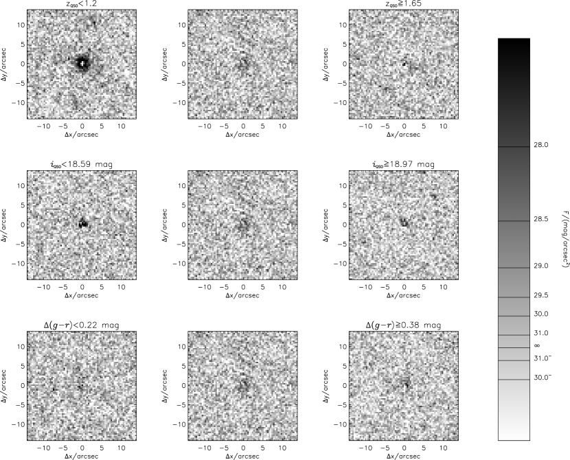
Figure 16.— The $i$-band stack images of reference QSOs in different disjoint bins in the $z_{QSO}$-$i_{QSO}$-$\Delta(g-r)$ parameter space. Only the central $30\times 30~{}\mathrm{arcsec}^{2}$ are reproduced, using a linear grey scale to map the intensity. The corresponding levels in mag arcsec^-2 are reported in the key bar on the right ($\infty$ means background level). The three images in the central column represent the same reference central bin in the parameter space, namely $1.2\leq z_{QSO}<1.65$, $18.59\leq i_{QSO}<18.97$, $0.22~{}\mathrm{mag}\leq\Delta(g-r)<0.38~{}\mathrm{mag}$. The left and right panels in each rows are bins where only one of the three parameters at time is varied with respect to the central reference bin, as indicated by the labels.

Let us now consider subsamples where we vary the range of each of the three parameters separately, to investigate their effect on the residuals of PSF subtraction. In the first upper row of fig. 16 we show the images of the low- ($z_{QSO}<1.2$, to the left) and the high- ($z_{QSO}<1.2$, to the right) QSO redshift subsamples, with the same $i_{QSO}$ and $\Delta(g-r)$ cuts as in the reference. Similarly, in the second row we make the $i_{QSO}$ vary (bright $i_{QSO}<18.59$ to the left and faint $i_{QSO}\geq 18.97$ to the right), while keeping fix the other two parameters as in the reference subsample; and finally in the third row the $\Delta(g-r)$ is varied (well matched star-QSO pairs to the left, $\Delta(g-r)<0.22$ mag, and poorly matched pairs to the right, $\Delta(g-r)\geq 0.38$ mag). The immediate conclusion that can be drawn from the analysis of fig.16 is that most of the SB excess around unabsorbed QSOs is produced by low redshift QSOs. Also, high redshift QSOs have no SB excess at all. The most logical explanation for this is that at low redshift we do detect the light of the QSO’s host galaxy, which drops below our detection limits at $z_{QSO}\gtrsim 1.5$. The lack of any significant dependence of the SB excess on either $\Delta(g-r)$ or $i_{QSO}$ shows that the color dependence of the PSF is well compensated by our algorithm (see §3.2) and that there are no serious deblending problems with fainter QSO being harder to deblend from neighboring faint stars or galaxies.

References

- Adelman-McCarthy et al. (2006) Adelman-McCarthy, J. K., et al. 2006, ApJS, 162, 38
- Bahcall & Spitzer (1969) Bahcall, J. N., & Spitzer, L. J. 1969, ApJ, 156, L63
- Baldry et al. (2004) Baldry, I. K., Glazebrook, K., Brinkmann, J., Ivezić, Ž., Lupton, R. H., Nichol, R. C., & Szalay, A. S. 2004, ApJ, 600, 681
- Bartelmann & White (2003) Bartelmann, M., & White, S. D. M. 2003, A&A, 407, 845
- Bender et al. (2001) Bender, R., et al. 2001, Deep Fields: Proceedings of the ESO Workshop Held at Garching, Germany, 9-12 October 2000, ESO ASTROPHYSICS SYMPOSIA. S. Cristiani, A. Renzini, and R.E. Williams Editors. Springer-Verlag, p. 96
- Bergeron & Boissé (1991) Bergeron, J., & Boisse, P. 1991, A&A, 243, 344
- Bergeron (1986) Bergeron, J. 1986, A&A, 155, L8
- Bergeron & Stasinska (1986) Bergeron, J., & Stasinska, G. 1986, A&A, 169, 1
- Bergeron et al. (1987) Bergeron, J., Kunth, D., & D’Odorico, S. 1987, A&A, 180, 1
- Bertin & Arnouts (1996) Bertin, E., & Arnouts, S. 1996, A&AS, 117, 393
- Blanton et al. (2003) Blanton, M. R., et al. 2003, ApJ, 592, 819
- Blanton et al. (2005) Blanton, M. R., Lupton, R. H., Schlegel, D. J., Strauss, M. A., Brinkmann, J., Fukugita, M., & Loveday, J. 2005, ApJ, 631, 208
- Bond et al. (2001) Bond, N. A., Churchill, C. W., Charlton, J. C., & Vogt, S. S. 2001, ApJ, 562, 641
- Bouché et al. (2006) Bouché, N., Lehnert, M. D., & Péroux, C. 2006, MNRAS, 367, L16
- Bowen et al. (2006) Bowen, D. V., et al. 2006, ApJ, 645, L105
- Brandt et al. (2001) Brandt, W. N., Hornschemeier, A. E., Schneider, D. P., Alexander, D. M., Bauer, F. E., Garmire, G. P., & Vignali, C. 2001, ApJ, 558, L5
- Bruzual & Charlot (2003) Bruzual, G., & Charlot, S. 2003, MNRAS, 344, 1000
- Calzetti et al. (1994) Calzetti, D., Kinney, A. L., & Storchi-Bergmann, T. 1994, ApJ, 429, 582
- Cardelli et al. (1989) Cardelli, J. A., Clayton, G. C., & Mathis, J. S. 1989, ApJ, 345, 245
- Churchill et al. (1999) Churchill, C. W., Mellon, R. R., Charlton, J. C., Jannuzi, B. T., Kirhakos, S., Steidel, C. C., & Schneider, D. P. 1999, ApJ, 519, L43
- Churchill et al. (2000) Churchill, C. W., Mellon, R. R., Charlton, J. C., Jannuzi, B. T., Kirhakos, S., Steidel, C. C., & Schneider, D. P. 2000, ApJS, 130, 91
- Churchill et al. (2005a) Churchill, C. W., Kacprzak, G. G., & Steidel, C. C. 2005a, IAU Colloq. 199: Probing Galaxies through Quasar Absorption Lines, 24
- Churchill et al. (2005b) Churchill, C., Steidel, C., & Kacprzak, G. 2005b, ASP Conf. Ser. 331: Extra-Planar Gas, 331, 387
- Churchill et al. (2006) Churchill, C. W., Kacprzak, G. G., Steidel, C. C., & Murphy, T. M. 2006, ApJ submitted
- Cristiani (1987) Cristiani, S. 1987, A&A, 175, L1
- Fried (1965) Fried, D. L. 1965, Optical Society of America Journal A, 55, 1427
- Fukugita et al. (1996) Fukugita, M., Ichikawa, T., Gunn, J. E., Doi, M., Shimasaku, K., & Schneider, D. P. 1996, AJ, 111, 1748
- Gabasch et al. (2004) Gabasch, A., et al. 2004, A&A, 421, 41
- Guillemin & Bergeron (1997) Guillemin, P., & Bergeron, J. 1997, A&A, 328, 499
- Heckman et al. (2000) Heckman, T. M., Lehnert, M. D., Strickland, D. K., & Armus, L. 2000, ApJS, 129, 493
- Heidt et al. (2003) Heidt, J., et al. 2003, A&A, 398, 49
- Hogg et al. (1997) Hogg, D. W., Neugebauer, G., Armus, L., Matthews, K., Pahre, M. A., Soier, B. T., & Weinberger, A. J. 1997, AJ, 113, 474
- Ivezić et al. (2002) Ivezić, Ž., et al. 2002, ASP Conf. Ser. 284: AGN Surveys, 284, 137
- Kacprzak et al. (2006) Kacprzak, G. G., Churchill, C. C., Steidel, C. C., & Murphy, M. T. 2006, ApJ submitted
- Kauffmann et al. (2003) Kauffmann, G., et al. 2003, MNRAS, 341, 54
- Lin & Mohr (2004) Lin, Y.-T., & Mohr, J. J. 2004, ApJ, 617, 879
- Lupton et al. (2001) Lupton, R., Gunn, J. E., Ivezić, Z., Knapp, G. R., & Kent, S. 2001, ASP Conf. Ser. 238: Astronomical Data Analysis Software and Systems X, 238, 269
- Mandelbaum et al. (2006) Mandelbaum, R., Seljak, U., Kauffmann, G., Hirata, C. M., & Brinkmann, J. 2006, MNRAS, 368, 715
- McQuade et al. (1995) McQuade, K., Calzetti, D., & Kinney, A. L. 1995, ApJS, 97, 331
- Ménard et al. (2005) Ménard, B., Zibetti, S., Nestor, D., & Turnshek, D. 2005, IAU Colloq. 199: Probing Galaxies through Quasar Absorption Lines, 86
- Mo & Miralda-Escude (1996) Mo, H. J., & Miralda-Escude, J. 1996, ApJ, 469, 589
- Nestor et al. (2003) Nestor, D. B., Rao, S. M., Turnshek, D. A., & Vanden Berk, D. 2003, ApJ, 595, L5
- Nestor et al. (2005) Nestor, D. B., Turnshek, D. A., & Rao, S. M. 2005, ApJ, 628, 637
- Pence (1999) Pence, W. 1999, ASP Conf. Ser. 172: Astronomical Data Analysis Software and Systems VIII, 172, 487
- Press et al. (1992) Press, W. H., Teukolsky, S. A., Vetterling, W. T., & Flannery, B. P. 1992, Cambridge: University Press, 1992, 2nd ed.
- Prochter et al. (2006) Prochter, G. E., Prochaska, J. X., & Burles, S. M. 2006, ApJ, 639, 766
- Rao et al. (2006) Rao, S. M., Turnshek, D. A., & Nestor, D. B. 2006, ApJ, 636, 610
- Richards et al. (2002) Richards, G. T., et al. 2002, AJ, 123, 2945
- Schneider et al. (2005) Schneider, D. P., et al. 2005, AJ, 130, 367
- Schlegel et al. (1998) Schlegel, D. J., Finkbeiner, D. P., & Davis, M. 1998, ApJ, 500, 525
- Smith et al. (2002) Smith, J. A., et al. 2002, AJ, 123, 2121
- Steidel & Sargent (1992) Steidel, C. C., & Sargent, W. L. W. 1992, ApJS, 80, 1
- Steidel et al. (1994) Steidel, C. C., Dickinson, M., & Persson, S. E. 1994, ApJ, 437, L75
- Steidel (1995) Steidel, C. C., 1995, QSO Absorption Lines, Proceedings of the ESO Workshop Held at Garching, Germany, 21 - 24 November 1994, edited by Georges Meylan. Springer-Verlag Berlin Heidelberg New York. Also ESO Astrophysics Symposia, 1995., p.139, 139
- Storchi-Bergmann et al. (1995) Storchi-Bergmann, T., Kinney, A. L., & Challis, P. 1995, ApJS, 98, 103
- White et al. (2006) White, R. L., Helfand, D. J., Becker, R. H., Glikman, E., & deVries, W. 2006, ArXiv Astrophysics e-prints, arXiv:astro-ph/0607335
- Wolf et al. (2003) Wolf, C., Meisenheimer, K., Rix, H.-W., Borch, A., Dye, S., & Kleinheinrich, M. 2003, A&A, 401, 73
- York et al. (2000) York, D. G., et al. 2000, AJ, 120, 1579
- York et al. (2006) York, D. G., et al. 2006, MNRAS, 367, 945
- Zibetti et al. (2004) Zibetti, S., White, S. D. M., & Brinkmann, J. 2004, MNRAS, 347, 556
- Zibetti et al. (2005a) Zibetti, S., Ménard, B., Nestor, D., & Turnshek, D. 2005, ApJ, 631, L105
- Zibetti et al. (2005b) Zibetti, S., White, S. D. M., Schneider, D. P., & Brinkmann, J. 2005, MNRAS, 358, 949