The correlation between the distribution of galaxies and 21cm emission at high redshifts

Abstract

Deep surveys have recently discovered galaxies at the tail end of the epoch of reionization. In the near future, these discoveries will be complemented by a new generation of low-frequency radio observatories that will map the distribution of neutral hydrogen in the intergalactic medium through its redshifted 21cm emission. In this paper we calculate the expected cross-correlation between the distribution of galaxies and intergalactic 21cm emission at high redshifts. We demonstrate using a simple model that overdense regions are expected to be ionized early as a result of their biased galaxy formation. This early phase leads to an anti-correlation between the 21cm emission and the overdensities in galaxies, matter, and neutral hydrogen. Existing Ly$\alpha$ surveys probe galaxies that are highly clustered in overdense regions. By comparing 21cm emission from regions near observed galaxies to those away from observed galaxies, future observations will be able to test this generic prediction and calibrate the ionizing luminosity of high-redshift galaxies.

1 Introduction

An important question that should be addressed by successful models of reionization concerns whether overdense or underdense regions become ionized first. In regions that are overdense, galaxies will be over-abundant for two reasons; first because there is more material per unit volume to make galaxies, and second because small-scale fluctuations need to be of lower amplitude to form a galaxy when embedded in a larger-scale overdensity (the so-called galaxy bias; see Mo & White 1996). Regarding reionization of the intergalactic medium (IGM), the first effect will be compensated by the increased density of gas to be ionized. Furthermore, the increase in the recombination rate in overdense regions will be counteracted by the galaxy bias in overdense regions. However the latter effects need not cancel, and could either lead to enhanced or delayed reionization in overdense regions.

The process of reionization also contains several layers of feedback. Radiative feedback heats the IGM and results in the suppression of low-mass galaxy formation (Efstathiou, 1992; Thoul & Weinberg 1996; Quinn et al. 1996; Dijkstra et al. 2004). This delays the completion of reionization by lowering the local star formation rate, but the effect is counteracted in overdense regions by the biased formation of massive galaxies. The radiation feedback may therefore be more important in low-density regions where small galaxies contribute more significantly to the ionizing flux.

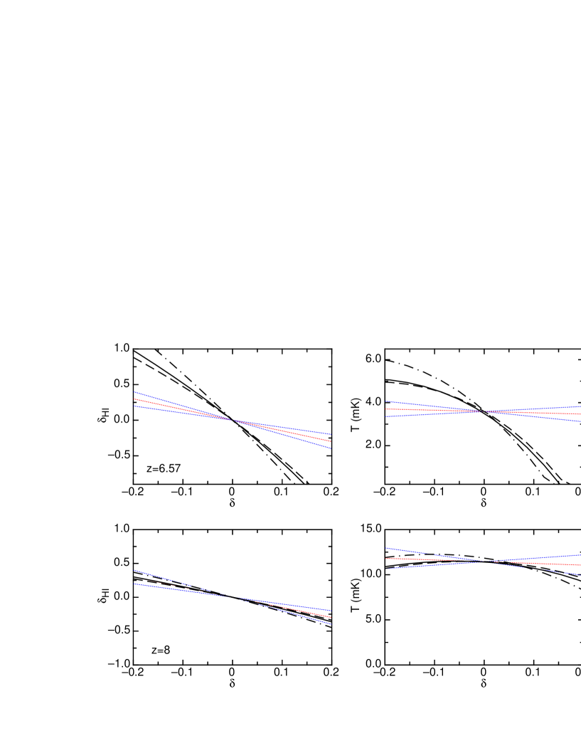
Figure 1: Left: Fluctuations in the hydrogen neutral fraction [$\delta_{\rm HI}\equiv x_{\rm HI}(\delta)/\langle x_{\rm HI}\rangle-1$] versus overdensity $\delta$ (for $R\gg R_{\rm min}$). The solid, dot-dashed and dashed lines represent values of $C=10$, $C=2$ and $C=20$. For comparison, we show three lines of slope $d\delta_{\rm HI}/d\delta=-0.5$, $-1.5$ and $-2.5$. Right: The dependence of the predicted brightness temperature ($T$) on overdensity. The solid, dot-dashed and dashed lines represent values of $C=10$, $C=2$ and $C=20$. For comparison, the three lines show Equation (1) with values of $\beta=-0.5$, -1.5 and -2.5. The upper and lower rows correspond to observations at $z=6.57$ and $z=8$ respectively.

In this paper we use a simple model to evaluate the relative significance of the above effects and compute the correlation between the local overdensity and quantities such as the hydrogen neutral-fraction, the brightness temperature of redshifted 21cm emission, and the overdensity of massive galaxies. In particular, we evaluate the prospects for finding whether reionization is enhanced or suppressed in overdense regions based on the combination of high redshift galaxy surveys and redshifted 21cm surveys.

For illustration, the problem may be parameterised by relating the neutral fraction [$x_{\rm HI}^{R}(\delta)$] in regions of linear overdensity $\delta$ (smoothed over spheres of large radius $R$), to the average neutral fraction ($x_{\rm HI}$) using a power-law with index $\beta(R)$

$$x_{\rm HI}^{R}(\delta)=x_{HI}\left(1+\delta\right)^{\beta(R)}\approx x_{HI}\left[1+\beta(R)\delta\right],$$ (1)

where we assume $\delta\ll 1$. The resulting deviation in the brightness temperature of a region of overdensity $\delta$ at $z\ga 6$ is

$$T(\delta) \approx 22\mbox{mK}x_{\rm HI}^{R}\left(1+\frac{4}{3}\delta\right)$$ (2)

$$\approx 22\mbox{mK}x_{HI}\left[1+\left(\frac{4}{3}+\beta(R)\right)\delta\right],$$

where we have assumed hydrogen in the IGM to have a spin temperature well in excess of the CMB temperature. In Equation (2) the pre-factor of 4/3 on the overdensity refers to the spherically averaged enhancement of the brightness temperature due to peculiar velocities in overdense regions (Bharadwaj & Ali 2005; Barkana & Loeb 2005). In a state where the ionization fraction in the IGM is independent of density, the value of the index is $\beta=0$ for all scales. If $\beta<0$, then ionization is enhanced in overdense regions. Conversely, reionization is suppressed in overdense regions if $\beta>0$. High redshift galaxies are preferentially located in large-scale regions with $\delta>0$. The departure of the mean 21cm brightness temperature in these regions from the average IGM provides the opportunity to measure the value of $\beta$, and hence to determine whether overdense or underdense regions were reionized first. In §2 we describe a simple model that predicts $\beta<0$. Regions of higher density should therefore be more ionized and possess reduced levels of fluctuations in redshifted 21cm emission. We later describe how the dependence of 21cm emission on overdensity could be extracted based on the fact that more massive galaxies populate higher density regions. Throughout the paper we adopt the set of cosmological parameters determined by WMAP (Spergel et al. 2006) for a flat $\Lambda$CDM universe.

2 Simple model for the correlation of 21cm emission with large-scale overdensity

Figure 2: The auto-correlation function of 21cm brightness temperature smoothed on different angular scales $\theta$. The four lines show the results at redshifts $z=6.5$ (solid), $z=7$ (short-dashed), $z=8$ (long-dashed) and $z=10$ (dot-dashed). The left and right panels correspond to clumping factors $C=10$ and $C=2$, respectively.

The evolution of the ionization fraction by mass $Q_{\delta,R}$ of a particular region of scale $R$ with overdensity $\delta$ (at observed redshift $z_{\rm obs}$) may be written as (Wyithe & Loeb 2003)

$$\frac{dQ_{\delta,R}}{dt} = \frac{N_{\rm ion}}{0.76}\left[Q_{\delta,R}\frac{dF_{\rm col}(\delta,R,z,M_{\rm ion})}{dt}\right.$$ (3)

$$\hskip 14.22636pt+\left.\left(1-Q_{\delta,R}\right)\frac{dF_{\rm col}(\delta,R,z,M_{\rm min})}{dt}\right]$$

$$- \alpha_{\rm B}Cn_{\rm H}^{0}\left(1+\delta\frac{D(z)}{D(z_{\rm obs})}\right)\left(1+z\right)^{3}Q_{\delta,R},$$

where $N_{\rm ion}$ is the number of photons entering the IGM per baryon in galaxies, $\alpha_{\rm B}$ is the case-B recombination co-efficient, $C$ is the clumping factor (which we assume, for simplicity, to be constant), and $D(z)$ is the growth factor between redshift $z$ and the present time. The production rate of ionizing photons in neutral regions is assumed to be proportional to the collapsed fraction $F_{\rm col}$ of mass in halos above the minimum threshold mass for star formation ($M_{\rm min}$), while in ionized regions the minimum halo mass is limited by the Jeans mass in an ionized IGM ($M_{\rm ion}$). We assume $M_{\rm min}$ to correspond to a virial temperature of $10^{4}$K, representing the hydrogen cooling threshold, and $M_{\rm ion}$ to correspond to a virial temperature of $10^{5}$K, representing the mass below which infall is suppressed from an ionized IGM (Dijkstra et al. 2004). In a region of co-moving radius $R$ and mean overdensity $\delta(z)=\delta D(z)/D(z_{\rm obs})$ [specified at redshift $z$ instead of the usual $z=0$], the relevant collapsed fraction is obtained from the extended Press-Schechter (1974) model (Bond et al. 1991) as

$$F_{\rm col}(\delta,R,z)=\mbox{erfc}{\left(\frac{\delta_{\rm c}-\delta(z)}{\sqrt{2\left(\left[\sigma_{\rm gal}\right]^{2}-\left[\sigma(R)\right]^{2}\right)}}\right)},$$ (4)

where $\mbox{erfc}(x)$ is the error function, $\sigma(R)$ is the variance of the density field smoothed on a scale $R$, and $\sigma_{\rm gal}$ is the variance of the density field smoothed on a scale $R_{\rm gal}$, corresponding to a mass scale of $M_{\rm min}$ or $M_{\rm ion}$ (both evaluated at redshift $z$ rather than at $z=0$). In this expression, the critical linear overdensity for the collapse of a spherical top-hat density perturbation is $\delta_{c}\approx 1.69$. The details of the galaxy bias and radiative feedback must be incorporated in order to compute how $F_{\rm col}$ and $C$ vary with $\delta$. Before proceeding, we stress that this model is intended to be illustrative only. While semi-analytic models can offer a picture of the global properties of reionization, the detailed processes must be modeled numerically using cosmological simulations (e.g. Zahn et al. 2006).

Figure 3: Left panel: The number counts of Ly$\alpha$ emitters as a function of observed luminosity $\mathcal{T}L_{\rm Ly}$. The data points are from the cumulative number counts of Kashikawa et al. (2006) for the SDF (incompleteness corrected). The solid line is the best fit model assuming Equations (7-8), with $\epsilon_{\rm dc}=0.38$ and $f_{\rm star}\mathcal{T}=0.24$. Right panel: contours of likelihood in the $f_{\rm star}\mathcal{T}$ versus $\epsilon_{\rm dc}$ plane at 14%, 26% and 64% of the maximum likelihood. These contours correspond to the 3, 2 and 1-sigma levels of a Gaussian distribution. The long and short dashed lines show lines of constant mass at $M=10^{10}M_{\odot}$ and $M=10^{11}M_{\odot}$ respectively.

Equation (3) may be integrated as a function of $\delta$ at the observed redshift. As an example, we find the value of $N_{\rm ion}$ that yields overlap of ionized regions at the mean density IGM by $z\sim 6$ (White et al. 2003). We then use the model to compute the filling fraction of ionized regions at $z=6.57$ (corresponding to the redshift of Ly$\alpha$ galaxy surveys discussed in the next section) and at a higher redshift of $z=8$. The results are shown in the left panels of Figure 1, where fluctuations in neutral fraction [$\delta_{\rm HI}\equiv x_{\rm HI}(\delta)/\langle x_{\rm HI}\rangle-1$] are plotted versus $\delta$. Results are shown assuming clumping factors of $C=10$ (solid lines), $C=2$ (dot-dashed lines), and $C=20$ (dashed lines). Here the overdensities correspond to length scales in the IGM that are significantly in excess of the length scale corresponding to the minimum mass (i.e. Figure 1 represents scales where $[\sigma_{\rm min}]^{2}-[\sigma(R)]^{2}\approx\sigma_{\rm min}^{2})$. Therefore while Figure 1 shows dependencies out to values of $\delta\sim 0.5$, such overdensities are rare on these large scales. We find that overdense regions are more highly ionized than underdense regions, implying that the bias of massive galaxies in overdense regions dominates over the increased recombination rate there. Figure 1 shows that fluctuations in the neutral fraction at a fixed overdensity (as measured at an observed redshift $z_{\rm obs}$) are smaller at earlier times. The reason is simply that the neutral fraction is larger at earlier times, so that fluctuations in ionization fraction result in smaller relative fluctuations in neutral fraction. The left panels of Figure 1 also show three lines of slope $d\delta_{\rm HI}/d\delta=-0.5$, $-1.5$ and $-2.5$. From comparison of these lines with our model prediction, we find that the value of $\beta$ in Equations (1) and (2) is around $\beta\sim-1.5$ at $z=8$ (for $C=10$), and is significantly steeper at lower redshifts or lower clumping factors. Figure 1 suggests that a sufficiently large clumping factor would result in an ionization fraction that was lower in overdense relative to underdense regions.

On the right hand panels of Figure 1 we plot the variation of predicted 21cm brightness temperature ($T$) with overdensity. Results are again shown assuming clumping factors of $C=10$ (solid lines), $C=2$ (dot-dashed lines) and $C=20$ (dashed lines). For comparison, the three lines show Equation (2) with values of $\beta=-0.5$, -1.5 and -2.5. At positive overdensities, we find a reduced neutral fraction. However in these regions, the neutral hydrogen present is at an increased overdensity. The brightness temperature of an overdense region is therefore reduced relative to the average by increased ionization, but increased relative to average by the higher gas density. Conversely the brightness temperature of an underdense region is increased relative to the average by reduced ionization, but decreased relative to average by the lower gas density. At large redshifts and/or clumping factor, we find that the sum of these effects results in a non-monotonic dependence of $T$ on $\delta$, with brightness temperature peaking near $\delta=0$.

On co-moving scales ($R$) sufficiently large that the variance in the density field remains in the linear regime, we are able to compute the auto-correlation function [$\xi_{T}(\theta)$] of brightness temperature smoothed with top-hat windows of angular radius $\theta=R/d_{\rm A}(z)$, where $d_{\rm A}$ is the angular diameter distance:

$$\xi_{T}(\theta) = \langle\left(T-\langle T\rangle\right)^{2}\rangle^{1/2}$$ (5)

$$= \left[\frac{1}{\sqrt{2\pi}\sigma(R)}\int d\delta\left(T(\delta)-\langle T\rangle\right)^{2}e^{-\frac{\delta^{2}}{2\sigma(R)^{2}}}\right]^{\frac{1}{2}},$$

where

$$\langle T\rangle=\frac{1}{\sqrt{2\pi}\sigma(R)}\int d\delta~{}T(\delta)e^{-\frac{\delta^{2}}{2\sigma(R)^{2}}},$$ (6)

and $\sigma(R)$ is the variance of the density field (at redshift $z$) smoothed on a scale $R$. The resulting auto-correlation functions are shown in Figure 2 assuming clumping factors of $C=10$ (left) and $C=2$ (right). The four curves correspond to redshifts of $z=6.5$, 7, 8 and 10, and demonstrate (in the case of $C=10$) that the amplitude of the auto-correlation function need not vary monotonically with redshift (or average neutral fraction).

3 The masses of Ly$\alpha$ emitters

We would like to determine whether the distribution of high redshift galaxies can be combined with redshifted 21cm maps to probe the correlations between the redshifted 21cm emission and galaxies, and hence between the ionization fraction and the large-scale overdensity. We concentrate on the case of Ly$\alpha$ emitting galaxies. In order to estimate the bias of Ly$\alpha$ emitting galaxies relative to the underlying density field, we first compare the observed abundance of Ly$\alpha$ emitters to a simple model in order to estimate their galaxy mass.

In the Subaru Deep Field (SDF) Kashikawa et al. (2006) find the density [$N_{\rm obs}(>\mathcal{T}L_{\rm Ly})$] of Ly$\alpha$ emitters brighter than an observed luminosity ($\mathcal{T}L_{\rm Ly}$) at $z=6.57$. Here $L_{\rm Ly}$ is the intrinsic luminosity of the emitter and $\mathcal{T}$ is the transmission of Ly$\alpha$ photons through the IGM. In the lowest luminosity bin, $\mathcal{T}L_{\rm Ly}=3\times 10^{42}$erg/s, and the density is $N_{\rm obs}(>\mathcal{T}L_{\rm Ly})=4\times 10^{-4}$Mpc^-3. The number counts from Kashikawa et al. (2006) are reproduced in Figure 3 (for the case where the densities are corrected for incompleteness). Our simple model for Ly$\alpha$ emitters (Haiman & Cen 2005) assumes the luminosity to be

$$\mathcal{T}L_{\rm Ly}=3\times 10^{42}\mbox{erg/s}\left(\frac{f_{\rm star}\mathcal{T}}{0.2}\right)\left(\frac{\epsilon_{\rm dc}}{0.1}\right)^{-1}\left(\frac{M}{10^{10}M_{\odot}}\right),$$ (7)

where $\epsilon_{\rm dc}$ is the duty-cycle, $f_{\rm star}$ is the star-formation efficiency, $M$ is the halo mass, and we have assumed the escape fraction of ionizing photons to be much smaller than unity. The density of Ly$\alpha$ emitters more luminous than $\mathcal{T}L_{\rm Ly}$ is given by

$$N(>\mathcal{T}L_{\rm Ly})=\epsilon_{\rm dc}\int_{M(L_{\rm Ly})}^{\infty}dM\frac{dn}{dM},$$ (8)

where $dn/dM$ is the Press-Schechter (1974) mass function (comoving number density per galaxy mass) with the modification of Sheth & Tormen (2002). For different combinations of $\epsilon_{\rm dc}$ and $f_{\rm star}\mathcal{T}$ we then generate model number counts $N(>\mathcal{T}L_{\rm Ly})$ using Equations (7-8). These number counts are compared to the data from the SDF. For each parameter set, a likelihood is produced $\mathcal{L}_{\rm Ly}(\epsilon_{\rm dc},f_{\rm star}\mathcal{T})=\Pi_{i=1}^{N}\exp{\left[-\frac{1}{2}(N_{{\rm obs},i}-N_{i})^{2}/\sigma_{i}^{2}\right]}$, where $N_{{\rm obs},i}$ and $N_{i}$ are evaluated in the $i$th observed luminosity bin ($i=1-9$), and $\sigma_{i}$ is the uncertainty in observed density at the $i$th luminosity bin. In the right panel of Figure 3 we show contours of the 14%, 26% and 64% of the maximum likelihood, corresponding to the 3, 2 and 1-sigma levels of a Gaussian distribution. The best fit model assuming Equations (7-8) has $\epsilon_{\rm dc}=0.38$ and $f_{\rm star}\mathcal{T}=0.24$. We expect a transmission of order unity (Dijkstra & Wyithe 2006). These values are unexpectedly high, however the model is degenerate over a wide range of parameter values. The best fit model is plotted over the data in the left panel of Figure 3. We are interested in the mass of Ly$\alpha$ emitters. In the right hand panel we show lines of constant mass corresponding to the lowest luminosity ($\mathcal{T}L_{\rm Ly}=3\times 10^{42}$erg/s) bin. The long and short dashed lines represent masses of $M=10^{10}M_{\odot}$ and $M=10^{11}M_{\odot}$ respectively. Based on these results we conclude that the halo masses of Ly$\alpha$ emitters in the SDF are larger than $10^{10}M_{\odot}$. In the remainder of this paper we show 21cm-galaxy correlations for both $M=10^{10}M_{\odot}$ and $M=10^{11}M_{\odot}$.

4 Cross-correlation of 21cm emission with galaxy properties

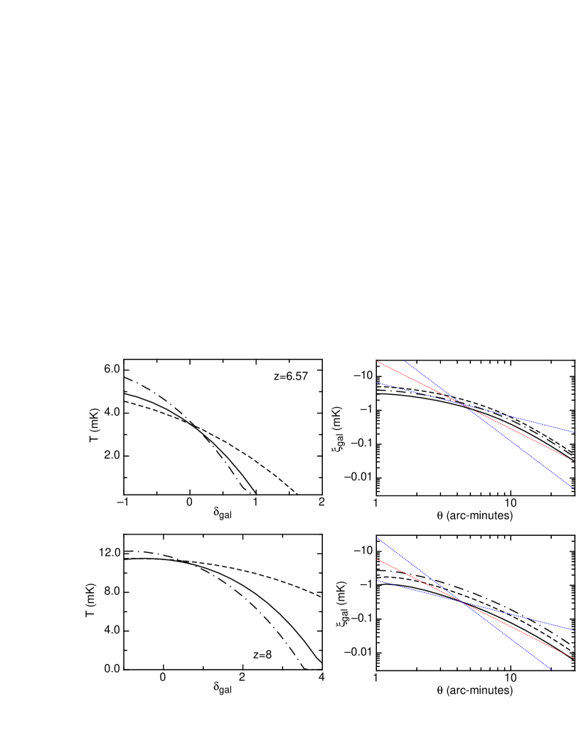
Figure 4: Left: 21cm brightness temperature as a function of $\delta_{\rm gal}$. Two values of galaxy mass are assumed for a clumping of $C=10$, $M=10^{10}M_{\odot}$ (solid line) and $M=10^{11}M_{\odot}$ (dashed line). The dot-dashed line shows $C=2$ with $M=10^{10}M_{\odot}$. Right: The cross-correlation function $\xi_{\rm gal}=\langle\delta_{\rm gal}\times(T-\langle T\rangle)\rangle$ for the IGM smoothed on various angular scales ($\theta$). The function is presented assuming $C=10$ for masses of $M=10^{10}M_{\odot}$ (solid line) and $M=10^{11}M_{\odot}$ (dashed line). The dot-dashed line represents $C=2$ with $M=10^{10}M_{\odot}$. The lines show power-laws of slope $d(\log\xi_{\rm gal})/d(\log\theta)=-1$, $-2$ and $-3$. The upper and lower rows correspond to observations at $z=6.57$ and $z=8$ respectively.

Next we discuss the cross-correlation between the number density of massive galaxies with 21cm emission. The observed overdensity of galaxies is simply $\delta_{\rm gal}=4/3\times b(M,z)\delta$, where $b(M,z)$ is the galaxy bias, and the pre-factor of 4/3 arises from a spherical average over the infall peculiar velocities (Kaiser 1987). The value of bias $b$ for a halo mass $M$ may be approximated using the Press-Schechter formalism (Mo & White 1996), modified to include non-spherical collapse (Sheth, Mo & Tormen 2001)

$$b(M,z)=1 + \frac{1}{\delta_{\rm c}}\left[\nu^{\prime 2}+b\nu^{\prime 2(1-c)}\right.$$ (9)

$$\hskip 28.45274pt-\left.\frac{\nu^{\prime 2c}/\sqrt{a}}{\nu^{\prime 2c}+b(1-c)(1-c/2)}\right],$$

where $\nu\equiv{\delta_{\rm c}^{2}}/{\sigma^{2}(M)}$, $\nu^{\prime}\equiv\sqrt{a}\nu$, $a=0.707$, $b=0.5$ and $c=0.6$. Here $\sigma(M)$ is the variance of the density field smoothed on a mass scale $M$ at redshift $z$. This expression yields an accurate approximation to the halo bias determined from N-body simulations (Sheth, Mo & Tormen 2001).

In the left-hand panels of Figure 4 we plot 21cm brightness temperature as a function of $\delta_{\rm gal}$. Results are shown for two values of galaxy mass, $M=10^{10}M_{\odot}$ (solid line) and $M=10^{11}M_{\odot}$ (dashed line) assuming $C=10$. We also show results for $M=10^{10}M_{\odot}$ assuming $C=2$ (dot-dashed line). The upper row of Figure 4 shows results for $z=6.57$, and the lower row for $z=8$.

The properties of the galaxy population correlate with the level of redshifted 21cm emission. These properties depend on the overdensity of the IGM whose typical fluctuation level is a function of scale. As a result the amplitude of the correlation between galaxy overdensity and 21cm emission will therefore also be dependent on angular scale. In the right panels of Figure 4 we plot the cross-correlation function

$$\xi_{\rm gal}(\theta) = \langle\delta_{\rm gal}\times(T-\langle T\rangle)\rangle$$ (10)

$$= \frac{1}{\sqrt{2\pi}\sigma(R)}\int d\delta\left(\delta_{\rm gal}\times(T-\langle T\rangle)\right)e^{\frac{-\delta^{2}}{2\sigma(R)^{2}}}$$

for the IGM smoothed on various angular scales, $\theta=R/d_{\rm A}$. Results are again shown for two values of galaxy mass, $M=10^{10}M_{\odot}$ (solid line) and $M=10^{11}M_{\odot}$ (dashed line) assuming $C=10$. As before we also show results for $M=10^{10}M_{\odot}$ assuming $C=2$ (dot-dashed line). The lines show power-laws of slope $d(\log|\xi_{\rm gal}|)/d(\log\theta)=-1$, $-2$ and $-3$ respectively. Since in these cases we find the brightness temperature to be lower in over-dense regions, we also find that massive galaxies correlate negatively with 21cm brightness temperature. The variance is lower on larger scales, and so the amplitude of the correlation is reduced.

The results shown in Figures 1, 2 and 4 are sensitive to the value of clumping factor. Weaker clumping leads to greater ionization in overdense regions, and hence a larger variation of ionization fraction with overdensity. This in turn leads to increases in the amplitudes of the auto-correlation and cross-correlation functions.

On scales of $\theta\sim 3^{\prime}$ the typical fluctuation in units of 1mK multiplied by the typical overdensity of galaxies is of order unity. In the next section we demonstrate that the brightness temperature around Ly$\alpha$ emitters at $z\sim 6$ should be sufficiently different from the average value to be detectable by the first generation of redshifted 21cm surveys.

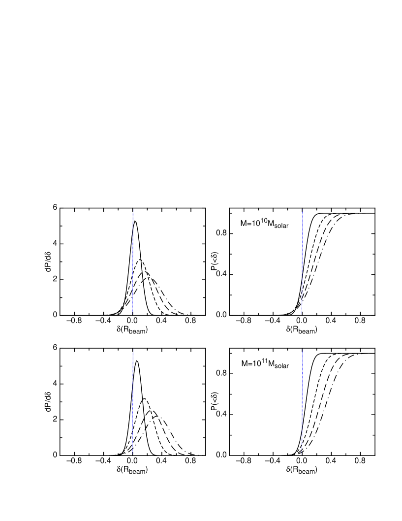
Figure 5: The differential (left) and cumulative (right) probability distributions for the large scale overdensity at the location of an observed Ly-alpha emitter. The solid, short-dashed, long-dashed and dot-dashed lines correspond to splitting up the Ly$\alpha$ survey into $N_{\rm bin}=1$, 2, 3 and 4 redshift bins. The upper and lower rows assume Ly$\alpha$ galaxy masses of $10^{10}M_{\odot}$ and $10^{11}M_{\odot}$ respectively.

5 Measurement of correlations between Ly$\alpha$ emitters and Fluctuating 21cm emission

The correlation between massive galaxies (which probe dense regions) and the 21cm signal (which traces the geometry of the neutral gas) will offer a direct probe of the process of reionization. The results of § 3 and § 4 suggest that Ly$\alpha$ emitters reside in massive galaxies at high redshift, and that overdensities in the number counts of these galaxies trace the more highly ionized regions. Observationally, Ly$\alpha$ surveys may provide the most straightforward comparison with 21cm maps for several reasons which we outline below. As a concrete example we consider the case of the Subaru Deep field and its comparison with an MWA-LFD (Mileura Wide Field Array-Low Frequency Demonstrator) field. We can estimate the sizes of fluctuations needed for detection by considering the uncertainty in the 21cm brightness averaged over synthesised beams which do or do-not contain Ly$\alpha$ emitting galaxies.

Radio telescopes measure images in data cubes and an instrument like the MWA-LFD will have much higher resolution (spatially) along the line-of sight than perpendicular to the line-of-sight. This allows for the option of binning in frequency space so that the data cube can have equal resolution in all three spatial dimensions. For an expected MWA-LFD resolution (beam radius) of $\theta_{\rm beam}=5$ arc-minutes, this corresponds to a region of $\pm 0.85$MHz or $\pm 1.6$ physical Mpc along the line-of-sight at $z=6.5$. A frequency interval of $2\times 0.85$MHz$=1.7$MHz at $z=6.5$ corresponds to a value of $\Delta z/(1+z)=0.008$, or a redshift range of $\Delta z=0.06$. For an efficient cross-correlation we would therefore like galaxy redshifts to be known to $\pm 0.03$, which requires spectroscopy. Surveys for Ly$\alpha$ emitters narrow down the redshift range initially via the use of narrow-band filters, and then find sources with a strong emission line, making spectroscopy attainable.

The characteristic lengths corresponding to the expected resolution of the MWA-LFD are well matched to the dimensions of surveys for Ly$\alpha$ emitting galaxies. For example, the SDF has a total area of 876 square arc-minutes. In this field the Subaru team found 50 Ly$\alpha$ emitter candidates. Spectra of 22 of these were obtained of which 16 were verified as high redshift galaxies, implying $N_{\rm Ly}\sim 36$ galaxies in this deep field. The line-of-sight dimension of the survey volume is set by the width of the narrow-band filter ($\Delta\lambda=132$Å), centered on a mean wavelength of $\lambda_{0}=9196$Å. This results in a field depth of $\Delta z=(1+z)\Delta\lambda/\lambda_{0}=0.11$, or $l=(cdt/dz)\Delta z\sim 5.9$Mpc. At $z\sim 6$ this depth is comparable to, but larger than the line-of-sight dimension corresponding to the expected MWA-LFD angular resolution. We may therefore divide the line of sight distance into a number of bins $N_{\rm bins}$, so that the size of each bin is $l_{\rm bin}=l/N_{\rm bin}$. We first define the angular scale that results in an angular beam radius $\theta_{\rm beam}=R_{\rm beam}/d_{\rm A}$, where $R_{\rm beam}=l_{\rm bin}/2$. This results in cylindrical volumes of space where the diameter equals the length of the cylinder. We are now able to find the number of such cylindrical regions in the SDF survey volume ($N_{\rm total})$, as well as the number containing galaxies [$N_{\rm gal}=N_{\rm Ly}/(1+\xi_{\rm Ly})$ where $\xi_{\rm Ly}$ is the excess probability above random of finding a second galaxy within a cylinder], and the number of cylinders not containing galaxies ($N_{\rm nogal}$).

We next discuss the response of a phased array to the brightness temperature contrast of the IGM. Assuming that calibration can be performed ideally, and that foreground subtraction is perfect, the root-mean-square fluctuations in brightness temperature are given by the radiometer equation

$$\langle\Delta T^{2}\rangle^{1/2}=\frac{\epsilon\lambda^{2}T_{\rm sys}}{A_{\rm tot}\Omega_{\rm b}\sqrt{t_{\rm int}\Delta\nu}},$$ (11)

where $\lambda$ is the wavelength, $T_{\rm sys}$ is the system temperature, $A_{\rm tot}$ the collecting area, $\Omega_{\rm b}$ the effective solid angle of the synthesized beam in radians, $t_{\rm int}$ is the integration time, $\Delta\nu$ is the size of the frequency bin, and $\epsilon$ is a constant that describes the overall efficiency of the telescope. We optimistically adopt $\epsilon=1$ in this paper. In units relevant for upcoming telescopes and at $\nu=200$MHz, we find (Wyithe, Loeb & Barnes 2005)

$$\Delta T = 7.5\left(\frac{1.97}{C_{\rm beam}}\right)\mbox{mK}\left(\frac{A}{A_{\rm LFD}}\right)^{-1}$$ (12)

$$\times \left(\frac{\Delta\nu}{1\mbox{MHz}}\right)^{-1/2}\left(\frac{t_{\rm int}}{100\mbox{hr}}\right)^{-1/2}\left(\frac{\theta_{\rm beam}}{5^{\prime}}\right)^{-2}.$$

Here $A_{\rm LFD}$ is the collecting area of a phased array consisting of 500 tiles each with 16 cross-dipoles [the effective collecting area of an LFD tile with $4\times 4$ cross-dipole array with 1.07m spacing is $\sim 17-19$m² between 100 and 200MHz (B. Correy, private communication)]. The system temperature at 200MHz will be dominated by the sky and has a value $T_{\rm sys}\sim 250$K. $\Delta\nu$ is the frequency range over which the signal is smoothed and $\theta_{\rm beam}$ is the size of the synthesized beam. The value of $\theta_{\rm beam}$ can be regarded as the radius of a hypothetical top-hat beam, or as the variance of a hypothetical Gaussian beam. The corresponding values of the constant $C_{\rm beam}$ are 1 and 1.97 respectively. Given the noise per synthesised beam, we can find the noise averaged in regions with and without galaxies as $\Delta T_{\rm gal}=\Delta T/\sqrt{N_{\rm gal}}$ and $\Delta T_{\rm nogal}=\Delta T/\sqrt{N_{\rm nogal}}$ respectively. The resulting uncertainty in brightness temperature between regions with and without galaxies is $\Delta T_{\rm diff}=\sqrt{(\Delta T_{\rm gal})^{2}+(\Delta T_{\rm nogal})^{2}}$.

The measurement of fluctuations in brightness temperature between over-dense and under-dense regions will require removal of emission from unresolved foreground objects. At a fixed frequency and on scales of a few arc-minutes, these foregrounds are believed to vary in amplitude at a level several orders of magnitude in excess of the expected 21cm signal (Di Matteo et al. 2002). However, the foregrounds are expected to have smooth power-law spectra, while 21cm emission from the IGM will fluctuate in both space and frequency. This smoothness should allow removal through subtraction of a continuum component, leaving fluctuations due to 21cm emission. However since the amplitude of the continuum will be different along each line of sight, we will be unable to determine its absolute level. Rather, the fluctuations in 21cm emission will need to be measured relative to the average continuum component along each line of sight (about which the fluctuations in brightness temperature will average to zero). This average continuum must be measured from a region of spectrum having finite length (the bandpass), and will therefore be determined only to an accuracy corresponding to fluctuations in the mean 21cm emission across the whole bandpass. For the MWA-LFD the bandpass will be 32MHz. We may estimate the level of uncertainty introduced through subtraction of the continuum by considering the variance of the density field in cylinders of radius a few arc-minutes (the synthesised beam size), and line of sight length corresponding to the band-pass. This variance can be shown to be around a few percent, which should be compared to the 10-20% representing the variance of the density field smoothed in spheres of radius a few arc-minutes. Therefore, while fluctuations in the continuum subtraction will add to the uncertainty in the measurement, they are substantially smaller than the 21cm fluctuations of interest.

In summary there are two aspects of the problem. First, there is the question of the distribution of overdensities (smoothed on the scale of the 21cm beam) in the IGM surrounding high redshift galaxies. The mean of this distribution must be significantly in excess of zero for any correlation of Ly$\alpha$ galaxies with large scale fluctuations in 21cm emission to be detectable. Second, there is the question of the sensitivity of the radio array, and the difference in average brightness temperature between regions (on the scale of the beam) that occupy or do not occupy galaxies. We treat each of these issues in turn.

Figure 6: Left panel: The measured error in brightness temperature between regions that contain or do not contain Ly$\alpha$ emitters as a function of the fraction of galaxies included. The four lines correspond to splitting up the Ly$\alpha$ survey into $N_{\rm bin}=2$, 3 and 4 redshift bins (short dashed, long dashed and dot-dashed respectively). Right panel: Comparison between the measurement error in $\delta T$ at the mean overdensity corresponding to observed Ly$\alpha$ emitters, with our model for the level of variation of temperature with overdensity ($C=10$). The errors have been plotted around the mean expected from the model. The 3 sets of points correspond to splitting up the Ly$\alpha$ survey into $N_{\rm bin}=2$, 3 and 4 redshift bins, and the values shown correspond to the minimum value of $\Delta T_{\rm diff}$ as a function of the fraction of the brightest galaxies used, $F_{\rm gals}$. The line styles are as per the left panel. The results were computed assuming experimental parameters that correspond to one SDF, combined with 1000 hours of integration on the MWA-LFD.

5.1 Ly$\alpha$ emitters as tracers of overdense regions

Strong clustering of massive sources in overdense regions implies that these sources should trace the higher density regions of IGM. In this section we compute the distribution of overdensities on a scale $R$ that are centered on galaxies of mass $M$. These overdensities are larger than average since galaxies preferentially form in overdense regions.

The likelihood of observing a galaxy at a random location is proportional to the number density of galaxies. At small values of large scale overdensity $\delta$, this density is proportional to $[1+\delta b(M,z)]$. More generally, given a large scale overdensity $\delta$ on a scale $R$, the likelihood of observing a galaxy may be estimated from the Sheth-Tormen (2002) mass function as

$$\mathcal{L}_{\rm g}(\delta)=\frac{(1+\delta)\nu(1+\nu^{-2p})e^{-a\nu^{2}/2}}{\bar{\nu}(1+\bar{\nu}^{-2p})e^{-a\bar{\nu}^{2}/2}},$$ (13)

where $\nu=(\delta_{\rm c}-\delta)/[\sigma(M)]$ and $\bar{\nu}=\delta_{\rm c}/[\sigma(M)]$. Here $\sigma(M)$ is the variance of the density field smoothed with a top-hat window on a mass scale $M$ at redshift $z$, and $a=0.707$ and $p=0.3$ are constants. Note that here as elsewhere in this paper, we work with overdensities and variances computed at the redshift of interest (i.e. not extrapolated to $z=0$). Equation (13) is simply the ratio of the number density of halos in a region of over-density $\delta$ to the number density of halos in the background universe. This ratio has been used to derive the bias for small values of $\delta$ (Mo & White 1996; Sheth, Mo & Tormen 2001). For example, in the Press-Schechter (1974) formalism we write

$$\mathcal{L}_{\rm g}(\delta) = (1+\delta)\left[\frac{dn}{dM}(\bar{\nu})+\frac{d^{2}n}{dMd\nu}(\nu)\frac{d\nu}{d\delta}\delta\right]\left[\frac{dn}{dM}(\bar{\nu})\right]^{-1}$$ (14)

$$\sim 1+\delta\left(1+\frac{\nu^{2}-1}{\sigma(M)\nu}\right)\equiv 1+\delta b,$$

where $(dn/dM)(\bar{\nu})$ and $(dn/dM)(\nu)$ are the average and perturbed mass functions, and $b$ is the bias factor. Utilising Bayes theorem, we find the a-posteriori probability distribution for the overdensity $\delta$ on the scale $R$ given the locations defined by a galaxy population. We obtain

$$\left.\frac{dP}{d\delta}\right|_{\rm gal}\propto\mathcal{L}_{\rm g}(\delta)\frac{dP_{\rm prior}}{d\delta},$$ (15)

where $\frac{dP_{\rm prior}}{d\delta}$ is a Gaussian of variance $\sigma(R)$.

In Figure 5 we show the differential (left panel) and cumulative (right panel) distributions of overdensity $\delta(R_{\rm beam})$ at the position of a Ly$\alpha$ emitting galaxy at $z=6.57$. The overdensities refer to a density distribution that has been smoothed on a scale $R_{\rm beam}$, and the Ly$\alpha$ emitters were assumed to have masses of $M=10^{10}M_{\odot}$ (upper row) and $M=10^{11}M_{\odot}$ (lower row). In each case the 4 lines correspond to values of $N_{\rm bins}=1$, 2, 3 and 4. The angular scales corresponding to these cases are $\theta_{\rm beam}=8.3^{\prime}$, $4.2^{\prime}$, $2.8^{\prime}$, and $2.1^{\prime}$. The means of these distributions are each greater than zero, with the departure greater in the case of smaller beam-size (which has larger intrinsic variance).

Not every galaxy will be observed in an overdense region. However we are interested in correlating the 21cm signal with galaxy position. The quantity of interest is therefore the distribution of the mean overdensity as measured using samples of $N_{\rm gal}$ galaxies. For $N_{\rm gal}=30$ and $M=10^{10}M_{\odot}$, we find that the mean overdensities sampled by galaxies are $\langle\delta\rangle_{\rm gal}=0.037\pm 0.015$, $0.10\pm 0.02$, $0.17\pm 0.03$, $0.22\pm 0.04$ for $N_{\rm bins}=1$, 2, 3 and 4 respectively. These values are each significantly in excess of zero. Mass conservation implies that regions devoid of galaxies must be underdense.

5.2 The sensitivity to brightness temperature fluctuations.

Results for $\Delta T_{\rm diff}$ are plotted in the left panel of Figure 6, assuming experimental parameters that correspond to one SDF, combined with 1000 hours of integration using the MWA-LFD. Here three lines are plotted corresponding to $N_{\rm bin}=2,3$ and 4 (bottom to top). The case of $N_{\rm bin}=1$ leads to a near absence of empty regions, and hence a large uncertainty. The Ly$\alpha$ emitters in the SDF cover an order of magnitude in luminosity. The noise is therefore plotted as a function of the fraction of the brightest galaxies used ($F_{\rm gals}$). The noise level can be reduced as the square-root of the integration time, in proportion to the collecting area or number of LFD units, and as the square-root of the number of SDF equivalents surveyed.

First let us suppose that the ionization fraction was uniform across the whole IGM. In this case the brightness temperature of regions surrounding galaxies would be greater than average by a factor $(1+\frac{4}{3}\langle\delta\rangle_{\rm gal})$. Similarly, those regions without Ly$\alpha$ emitters have $\langle\delta\rangle_{\rm nogal}<0$, and hence brightness temperatures that are lower than average by a factor $(1+\frac{4}{3}\langle\delta\rangle_{\rm nogal})$. We define the difference in brightness temperature between regions that contain and do not contain galaxies to be $\delta T$. The intrinsic (i.e. uniform ionization fraction) difference in brightness temperature between regions containing and not containing galaxies would therefore be

$$\delta T_{\rm int} = 22\mbox{mK}x_{\rm HI}\frac{4}{3}\left(\langle\delta\rangle_{\rm gal}-\langle\delta\rangle_{\rm nogal}\right)$$ (16)

$$\approx 4\mbox{mK}\left(\frac{\langle\delta\rangle_{\rm gal}-\langle\delta\rangle_{\rm nogal}}{0.3}\right)\left(\frac{x_{\rm HI}}{0.5}\right),$$

where $x_{\rm HI}$ is the average neutral fraction. This offset must be subtracted from any measured difference to find the difference in ionization state between over and under-dense regions. Equation (16) represents a value of $\delta T$ corresponding to an exponent of $\beta=0$ in the relation between overdensity and neutral fraction (see Equation 1).

From Equation (2) we find the uncertainty ($\Delta\beta$) in the exponent $\beta$ given an uncertainty in the brightness temperature ($\Delta T_{\rm diff}$) of the overdense regions

$$\Delta\beta\sim 0.25\left(\frac{\Delta T_{\rm diff}}{1\mbox{mK}}\right)\left(\frac{x_{\rm HI}^{R}}{0.5}\right)^{-1}\left(\frac{\langle\delta\rangle_{\rm gal}-\langle\delta\rangle_{\rm nogal}}{0.4}\right)^{-1}.$$ (17)

Figure 6 suggests that $\Delta T_{\rm dif}\sim 1$mK will be achievable with first generation instruments, combined with Ly$\alpha$ surveys of comparable size to those already performed. Given a measured uncertainty of $\Delta T_{\rm diff}\sim 1$mK, we can determine the exponent $\beta$ to $\Delta\beta=\pm 0.25$. This implies that we could easily tell the difference between reionization scenarios that predict $x_{\rm HI}\propto(1+\delta)^{-3}$ (i.e. the relation similar to that implied by our model), and a scenario where ionization was uniform with $x_{\rm HI}\propto const.$

Finally, as an example, we compare the expected brightness temperature noise and overdensity estimates (for experimental parameters that correspond to one SDF, combined with 1000 hours of integration using the MWA-LFD) to our model calculation of brightness temperature as a function of large scale overdensity (with $C=10$). Three curves are shown in the right panel of Figure 6, with mock data points showing the estimated error over-plotted for comparison (here the error bars have been computed for the value of $F_{\rm gals}$ that provides the smallest value of $\Delta T_{\rm diff}$). The three sets of points and curves correspond to splitting up of the Ly$\alpha$ survey into $N_{\rm bin}=2$, 3 and 4 redshift bins. The model curves have been computed assuming a scale for the overdensities that corresponds to the beam size ($R_{\rm beam}$) in each case. Note that where $N_{\rm bins}$ is smaller ($\sim 2$), the beams containing galaxies fill roughly half of the survey volume, so that $\langle\delta\rangle_{\rm gal}\approx-\langle\delta\rangle_{\rm nogal}$. Conversely, where $N_{\rm bins}$ is larger, the beams containing galaxies fill a small fraction of the survey volume. In this case $\langle\delta\rangle_{\rm gal}>-\langle\delta\rangle_{\rm nogal}$. This example shows that even at this late stage of reionization, first generation surveys will be able to detect the correlation of galaxies with 21cm emission. In the future, larger surveys and instruments will allow substantial improvements. For example, an array with 10 times the MWA-LFD collecting area, combined with 4 SDF’s would reduce the uncertainty in $\beta$ by a factor of $\sim 20$.

6 Summary

In this paper we have calculated the expected cross-correlation between the distribution of galaxies and the intergalactic 21cm emission at high redshifts. We constructed a simple model for reionization that accounts for both galaxy bias and an enhanced recombination rate in overdense regions, and used this model to compute the ionization fraction as a function of large scale overdensity in the IGM. Our model predicts that overdense regions will be ionized early as a result of their biased galaxy formation. This early phase of reionization in overdense regions leads to anti-correlations between the 21cm emission and the overdensity of baryons, and between the 21cm emission and the overdensity of neutral hydrogen. In addition, because galaxies are biased towards overdense regions, our model also predicts an anti-correlation between 21cm emission and the galaxy population.

To explore the detectability of any correlation between 21cm emission and galaxy properties, we also constructed a simple model for the Ly$\alpha$ emission corresponding to a dark-matter halo of a given mass, and hence for the Ly$\alpha$ luminosity function. We compared this model to an existing Ly$\alpha$ survey in the Subaru Deep Field. Through this comparison we demonstrated that current surveys probe galaxy masses that are larger than $10^{10}M_{\odot}$. Due to their biased formation, galaxies of this mass are highly clustered in overdense regions of the IGM. We have shown that by comparing 21cm emission from regions near observed galaxies to those away from observed galaxies, future redshifted 21cm observations will be able to test the generic prediction that overdense regions are reionized first.

Acknowledgments The research was supported by the Australian Research Council (JSBW) and Harvard University grants (AL).

References

- Barkana & Loeb (2005) Barkana, R., & Loeb, A. 2005, ApJL, 624, L65
- Bharadwaj & Ali (2005) Bharadwaj, S., & Ali, S. S. 2005, MNRAS, 356, 1519
- Bond et al. (1991) Bond, J. R., Cole, S., Efstathiou, G., & Kaiser, N. 1991, ApJ, 379, 440
- (4) Dijkstra, M., Haiman, Z., Rees, M. J., & Weinberg, D. H., Astrophys. J., 601, 666-675 (2004)
- (5) Dijkstra, M., Wyithe, J.S.B, 2006, MNRAS, in press
- Di Matteo et al. (2002) Di Matteo, T., Perna, R., Abel, T., & Rees, M. J. 2002, ApJ, 564, 576
- (7) Efstathiou, G., Mon. Not. R. Astron. Soc., 256, 43-47 (1992)
- Haiman & Cen (2005) Haiman, Z., & Cen, R. 2005, ApJ, 623, 627
- (9) Kaiser, N. 1987, MNRAS, 227, 1
- Kashikawa et al. (2006) Kashikawa, N., et al. 2006, ApJ, 648, 7
- Mo & White (1996) Mo, H. J., & White, S. D. M. 1996, MNRAS, 282, 347
- (12) Press, W., Schechter, P., 1974, ApJ., 187, 425
- (13) Quinn, T., Katz, N., & Efstathiou, G., 278, L49-L54 (1996)
- (14) Sheth, R., Tormen, G., 2002, MNRAS, 321, 61
- Sheth et al. (2001) Sheth, R. K., Mo, H. J., & Tormen, G. 2001, MNRAS, 323, 1
- (16) Spergel et al., 2006, astro-ph/0603449
- (17) Thoul, A. A., & Weinberg, D. H., Astrophys. J., 465, 608-116 (1996)
- (18) White, R., Becker, R., Fan, X., Strauss, M., 2003, Astron J., 126, 1
- (19) Wyithe, J. S. B, Loeb, A., 2003, ApJ, 586, 693
- Wyithe et al. (2003) Wyithe, J. S. B., Loeb, A., Barnes, D.G., 2005, ApJ, 634, 715
- (21) Zahn, O., et al., 2006, astro-ph/0604177