The end of the galactic cosmic ray spectrum
Abstract
We discuss the region of transition between galactic and extragalactic cosmic rays. The exact shapes and compositions of these two components contains information about important parameters of powerful astrophysical sources and the conditions in extragalactic space as well as for the cosmological evolution of the sources of high energy cosmic rays. Several types of experimental data, including the exact shape of the ultrahigh energy cosmic rays, their chemical composition and their anisotropy, and the fluxes of cosmogenic neutrinos have to be included in the solution of this problem.
1 INTRODUCTION
In view of the expected high experimental statistics from the Auger Observatory [1] the interest in the transition from galactic to extragalactic cosmic rays has increased significantly. It is now a standard belief that above some high energy of order 1019 eV all observed cosmic rays should come from extragalactic sources because they cannot be contained in the Galaxy long enough to be accelerated [2]. For the rest of this paper we shall assume that the Ultra-High Energy Cosmic Rays (UHECR) are accelerated at powerful astrophysical objects.
Extragalactic cosmic rays would lose energy in propagation from their sources to us if their sources are isotropically and homogeneously distributed in the Universe. The main energy loss process is the photoproduction interaction in the microwave background (MBR) that causes the GZK effect, the steepening of the cosmic ray spectrum above 61019 eV [3]. Several fits of the existing experimental data have been published in recent years that derived different values of the most important astrophysical and cosmological parameters: the acceleration (injection in terms of cosmic ray propagation) energy spectrum of these particles and the maximum acceleration energy, their chemical composition and the cosmological evolution of their astrophysical sources. In the assumption that most of UHECR are protons injection spectra as different as E-2.7 [4] and E-2.0 [5] and cosmological evolution of the type with values from 0 to 3 have been obtained.
Other attempts [6, 7, 8] have assumed that extragalactic cosmic rays have at their sources the same mixed chemical composition as the low energy galactic cosmic rays. In such a case the main energy loss process is the disintegration of the heavy nuclei mostly in interactions in MBR. Hadronic interactions become important only after the energy per nucleon exceeds the photoproduction threshold. The fits of the observed cosmic rays spectrum under this assumption gives an intermediate injection spectrum.
In all these attempts the fits of the observations show the end of the galactic cosmic rays spectrum which is obtained by subtraction of the propagated extragalactic spectrum from the experimentally observed one. This process gives some limits of the astrophysical parameters [9] when the subtraction gives unphysical negative values.
An important and interesting question is what such models predict for the chemical composition of UHECR, which for our purposes we shall define as cosmic rays of energy above 1018 eV. The assumption that extragalactic cosmic rays are protons obviously lead to a composition that becomes very light at GZK and super-GZK energies. Under the assumption that extragalactic cosmic rays have a mixed composition the conclusions are more complicated and the question of the highest acceleration energy is more important.
In terms of high energy astrophysics the location of the transition region can be used to estimate the strength of the cosmic ray sources in different types of astrophysical objects, from spiral galaxies like our own to Active Galactic Nuclei (AGN). In our current understanding the acceleration spectra depend on the strength of astrophysical shocks and the maximum acceleration energy is a function of the magnetic field strength and fluctuations . Other important parameters are the cosmological evolution of the UHECR sources and the strength of the extragalactic magnetic fields around the sources and the average magnetic field in the cosmologically nearby Universe.
We shall discuss several types of data and their predictions in different models: UHECR spectra and chemical composition, the anisotropy in this energy range, and the production of cosmogenic [10] neutrinos by extragalactic cosmic rays.
2 UHECR ENERGY SPECTRA
Figure 1 compares two different fits of the extragalactic cosmic ray spectra in the assumption that they are purely protons and that their differential acceleration spectrum is a power law . The experimental data are from AGASA [11] and HiRes [12] and are normalized to each other at 1019 eV. Since we are now only interested in the shape of the spectrum the exact differential flux at the normalization points is not important. It is obvious that the two experimental measurements agree well with each other on the shape of the energy spectrum with exception of the AGASA events above 1020 eV. The most recent analysis of the AGASA data, presented at this conference [13] decreases the energy assignment of the AGASA data by 10-15% and makes the spectrum closer to that of HiRes.
Fit a [4] derives an injection spectrum with = 1.7. The dip at about 1019 eV is due to the transition of proton energy loss to Bethe-Heitler pair production to purely adiabatic loss as predicted by Berezinsky&Grigorieva [14]. The model does not need any contribution from galactic cosmic rays to describe the observed cosmic ray spectrum down to 1018 eV. There is also no need for cosmological evolution of the extragalactic cosmic ray sources, although some source evolution can be accommodated with a slight change of . The model predicts purely proton composition of the extragalactic cosmic rays and does not work as well as shown in Fig. 1 if more than about 10% of the cosmic rays at the source are nuclei heavier than H.
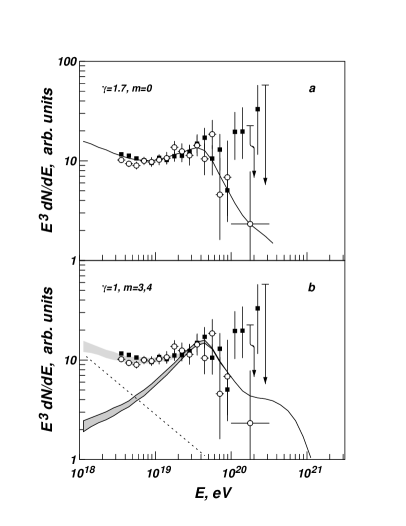
Fit b [5] does need contribution from galactic sources with spectrum that extends well above 1019 eV. The extragalactic contribution is shown for two different cosmological evolutions with = 3 (as used in Ref. [5]) and 4 (upper edge of the shaded area). The influence of the cosmological evolution on the cosmic ray propagation is modest because no protons injected at redshifts higher than 0.4 arrive at Earth with energy above 1019 eV independently of their initial energy.
Obviously these two models predict very differently the end of the galactic cosmic ray spectrum. In model a the galactic cosmic ray sources do not need to accelerate particles above 1018 eV. In model b they should be able to reach energies higher by one and a half orders of magnitude. This would affect very strongly the expected cosmic ray composition, as it will be discussed in the next Section.
The assumption that extragalactic cosmic rays have a mixed composition at acceleration gives somewhat intermediate results for the injection spectrum of UHECR [6, 7, 8]. The spectrum that fits the observation best has values between 1.2 and 1.4. The chemical composition of cosmic rays at Earth is also different and obviously depends on the source composition.
3 CHEMICAL COMPOSITION
If the assumption that extragalactic cosmic rays are of mixed composition similar to that of low energy galactic cosmic rays is correct, that would change our perception for the energy dependence of the cosmic ray chemical composition. Before examining it let me first state that we are discussing the composition in terms of total energy per nucleus, not the composition in terms of energy per nucleon as it is usually presented at energies between 1 and 100 GeV/nucleon.
Since we believe that galactic cosmic rays are accelerated in stochastic processes at astrophysical shocks (as they are in all models except in the Dar&DeRujula cannonball model [15, 16]) we expect cosmic ray nuclei to have maximum acceleration energy proportional to their rigidity, i.e. momentum/charge. Similar dependence comes out if the knee of the cosmic ray spectrum is due to leakage out of the Galaxy. The expectation is then that as soon as the maximum acceleration energy for hydrogen is approached the chemical composition starts becoming heavier - the maximum acceleration energy for He is higher by a factor of 2 (factor of 4 in the Dar&DeRujula model).
At the approach of galactic cosmic rays become purely iron nuclei and this is supposed to be the cosmic ray composition when the transition from galactic to extragalactic sources begins to happen. The measurements of the Kascade experiment [17] heavily support such behavior. Figure 2 shows the predicted composition as a function of the total energy per nucleus in the transition region in the classical cosmic ray units of . This is very appropriate when the detection is through air showers with logarithmic sensitivity to both energy and composition.
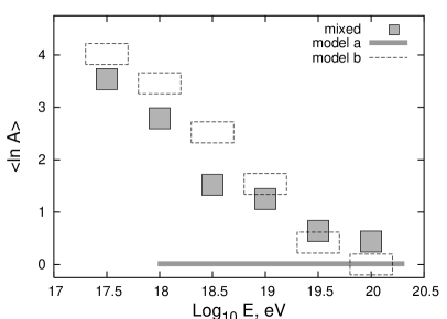
Model a presents the easiest case to explain. All composition changes happen below 1018 eV. We do not plot the composition below that energy as it is not very well defined. The results for the other two models are presented using our own understanding of them. For model b we assume that at 1017.5 eV all cosmic rays are iron and assign value of 4. At higher energy we use the fraction of galactic cosmic rays to iron nuclei and thus calculate the corresponding value. For the mixed composition we use Fig. 3 of Ref. [7] where the cosmic ray composition at Earth is plotted for =1.3 and is given as 1020.5 eV.
Surprisingly the difference in the energy dependence of of model b and of the mixed composition model is not that big, although in the model b case the composition only consists of a combination of Fe and H, and in the mixed composition case we have five groups of nuclei. Distinguishing between these two models depends on the experimental sensitivity. If the composition measurement uses the shower depth of maximum as a function of the total energy of the shower, as done in fluorescence experiments, the error bars shown in Fig. 2 are approximately correct for of about 50 g/cm2. A better sensitivity should be able to distinguish between a two component composition of model b and the five component mixed composition model.
Model a gives a very different picture, at least above 1018 eV, where the composition is purely Hydrogen. It is definitely distinguishable from the other two models. The prediction that the composition does not change above 1018 eV and is very light is supported by the HiRes measurement [18]. What is the exact meaning of light composition is not known because of the differences between the hadronic interaction models used for data analysis.
On the other hand, other experiments support a much milder energy dependence of the cosmic ray chemical composition, that is more in line with the prediction of of models b and that of mixed extragalactic cosmic ray composition.
4 ANISOTROPY
Low energy cosmic rays diffuse in the magnetic fields of the Galaxy and lose memory of the location of their sources. The anisotropies are very small, well below 1% and are difficult to measure. The measurement of a small anisotropy with air shower experiments requires an exact knowledge of the experimental acceptance and of the lifetime of the shower array.
At higher energy things are supposed to change as the cosmic ray rigidity increases and their diffusion in the Galaxy becomes faster. The first question we still cannot answer is of the rigidity (energy) dependence of the cosmic ray diffusion coefficient. From the ratio of secondary to primary cosmic rays an energy dependence of is derived. If this dependence is extended by seven orders of magnitude then galactic UHE protons should show very strong anisotropy that is not observed. The two spots with increased cosmic ray flux identified by the AGASA group [19] (one in the general direction of the Galactic center and one in the direction of Orion) are not confirmed by other experiments. Theoretically we expect Kolmogorov turbulence in the Galaxy, that should under some circumstances give energy dependence.
One way to explain the low anisotropy in the beginning of the transition region is to assume that all galactic cosmic rays are heavy nuclei. If they were indeed heavy nuclei the average particle rigidity would significantly decrease and would maintain the high isotropy of the galactic cosmic rays. In the transition region, however, the cosmic ray chemical composition becomes lighter and correspondingly we expect to see some degree of anisotropy.
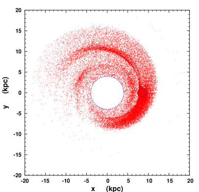
Figure 3 shows the location of the sources of cosmic ray protons that reach the Earth in a propagation calculation. The source distribution is assumed to be where is the galactocentric distance. There are no sources inside the 4 kpc circle. Cosmic rays are isotropically injected in the galactic plane on a spectrum with energies between 41017 and 21018 eV. The magnetic field model is BSS with random field and a magnetic dipole in the center of the Galaxy. The Earth is approximated by a sphere of radius 1 kpc to speed the calculation.
The figure shows the general behavior of protons in this energy range. They do not diffuse, rather follow the magnetic field lines. Because of the magnetic turbulence the protons occasionally jump from one magnetic field line to another and may change the direction of their propagation depending on the pitch angle.
When these protons arrive at Earth their arrival direction does not point at their source, they have rather a distribution that peaks in the direction of the local field line. Since we expect higher source density inside the solar circle, the expected anisotropy may peak in the general direction of Orion. Exercises like that one do create relatively strong anisotropy, much higher than observed.
One may complain that in Fig. 3 we are looking at particles that are accelerated in the galactic plane while in the case of extragalactic protons we will be dealing with particles that isotropically enter into the Galaxy and may not create any anisotropy. The truth is that calculations like the one that generated Fig. 3 show that protons of energy above 1016 eV emitted in the galactic plane leave the Galaxy much easier in the direction of the galactic poles that after propagation parallel to the galactic plane. In the entrance of the Galaxy we would expect the same effect - more extragalactic protons should arrive from absolute high galactic latitude than from low one.
This would not be the classical anisotropy that surveys the arrival direction as a function of the galactic longitude, but it should still be significant effect. The details of the effect depend strongly on the galactic magnetic field model [20] and on details of the calculation such as the dimension of the ‘Earth’ in the calculation and of the propagation step size.
I am convinced that in the case of high experimental statistics the anisotropy in the transition region between galactic and extragalactic cosmic rays deserves a careful study. A part of it is theoretical. We should propagate particles of different rigidity in the Galaxy and attempt to understand their general behavior. Analytic solutions of the diffusion equation are not any more suitable for this problem. Particle trajectory has to be numerically solved, most likely in a Monte Carlo fashion and in detailed enough magnetic field models. Such models should be tested to match analytic calculations when applied to the appropriate simplified models.
5 COSMOGENIC NEUTRINOS
Cosmogenic neutrinos are produced in the same photoproduction interactions of the UHECR protons that create the GZK effect. They were first proposed by Berezinsky&Zatsepin in 1969 [10] and were the subject of many calculations afterward. Cosmogenic neutrinos are often considered a ‘guaranteed source’ of ultrahigh energy neutrinos. They are indeed guaranteed, since we know UHECR exist, but their flux is unknown.
An essential quality of neutrinos is that they have a low interaction cross section. This makes neutrino detection a difficult problem that requires huge detectors of at least km3 scale. Such detectors are now in the stage of planning [21] and construction [22, 23]. The question of the cosmogenic neutrino flux and of its relation to other data from ultra-high astrophysics experiment is very timely.
The low interaction cross section is not only a deficiency. While protons emitted at redshifts exceeding 0.4 do not reach us with energy above 1019 eV the cosmogenic neutrino production peaks at redshifts exceeding 2 for cosmological evolution of the UHECR sources. This is the main link between the extragalactic UHECR and cosmogenic neutrinos. The detection of cosmogenic neutrinos may help the degeneracy in modeling of the extragalactic cosmic rays spectra shown in Fig. 1.
The point is that models that use flat cosmic ray injection spectrum and require strong cosmological evolution of the UHECR sources, such as model b would produce significantly more cosmogenic neutrinos than steep injection spectrum models with no cosmological evolution. Such a comparison between the two models is shown in Figure 4.
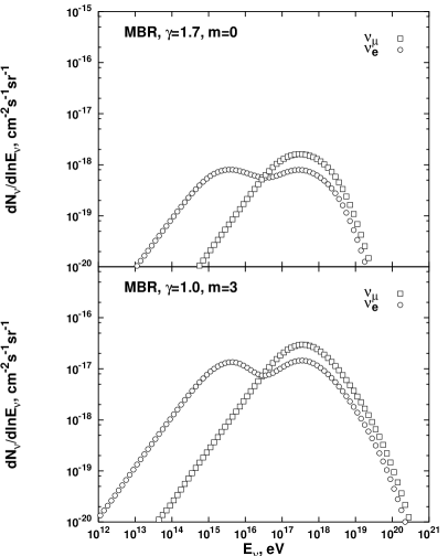
The figure shows cosmogenic neutrino fluxes generated by proton interactions in MBR with the injection spectrum and cosmological evolution of the two models as indicated in the two panels. The injection spectra of the two models are normalized to the UHECR differential flux at 1019 eV. Before discussing the magnitude of the two fluxes I want to attract your attention to the flux of electron neutrinos and antineutrinos that exhibits two maxima separated by about two orders of magnitude of energy. The higher energy one is due to the decay final state and consists mostly of electron neutrinos. It peaks at the same energy where and do. The lower energy maximum is due to electron antineutrinos from neutron decay. Comparison between the neutron interaction length in MBR and their decay length show that all neutrons of energy below 1020.5 eV decay rather than interact.
Model b generates much higher cosmogenic neutrino fluxes than model a because of two reasons that contribute roughly the same increase of the cosmological neutrinos. Firstly, it uses much flatter injection spectrum which means equal amount of energy per decade. It thus contains many more particles above the photoproduction interaction threshold with in the MBR is about 310 eV and, of course, decreases as .
The other reason is that model b employs a strong cosmological evolution of the cosmic ray sources. This increases by the number of particles injected at redshift of 2, but in addition increases by a factor of three the number of particles above the interaction threshold. This way the total neutron flux is increased by the cosmological evolution of the sources by a factor of five.
The difference in the peak values of the cosmological neutrinos generated by the two models is more than one order of magnitude. In practical terms this means that model b generates fluxes that are in principle detectable by IceCube at the rate of roughly less than one event per year, while model a generates undetectable fluxes of cosmogenic neutrinos in km3 detectors.
Ice and water neutrino detectors are generally not very suitable for cosmogenic neutrino detection. Much better strategies for these UHE neutrinos are the radio and acoustic detectors that have very high detection threshold, but also will have higher effective volume. The other option are giant air shower arrays such as Auger, that can reach effective volume of 30 km3 and, with sufficiently low threshold (1018 eV) could detect several events per year.
Cosmogenic neutrinos are also generated in the mixed composition scenario [25, 26]. Since the major energy loss process is the disintegration of heavy nuclei, the main flux component of from neutron decay. The flux exceeds by a factor of 5 the sum of the neutrino fluxes of all other flavors in Ref. [26]. The absolute magnitude depends again mainly on the injection spectrum and the cosmological evolution of the sources.
5.1 Production in the infrared/optical background
The difference between different models is somewhat decreased when photon fields different from MBR are considered. Several calculations that include the infrared/optical background (IRB) have been performed. The number density of IRB is of order 1 and varying by about a factor of 2 in different models, but its energy spectrum extends to energies as high as and exceeding 1 eV. What that means is that extragalactic particles of much lower energy would interact in IRB and will generate neutrinos. Reference [27] shows the neutrino yields generated by protons of energy as low as 1018 eV. This yield is small but has to be weighted by the much higher number of particles at that energy - almost 1,000 higher that that of 31019 eV for a flat injection spectrum. A more recent calculation that also includes UV photons [28] employs interactions of 1017 eV nucleons that have to be weighted still higher.
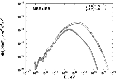
Figure 5 shows the cosmogenic neutrino fluxes from interactions in the MBR and IRB [27] by the two models. The difference in the peak values is now slightly less than a factor of three. The steep injection spectrum model a has significantly more protons that interact in the IRB and for that reason partially compensates for the lack of cosmological evolution of the sources. On the other hand, since the average neutrino energy is substantially lower and the neutrino interaction cross section increases with energy, the event rates produced by the two models would not change much. If one uses steep injection spectrum combined with an appropriate cosmological evolution of the sources that inclusion of the IRB target makes a big difference.
6 DISCUSSION
The transition region between galactic and extragalactic cosmic rays is currently not very well defined and studied. It has a significant astrophysical importance, because the energy content of the extragalactic cosmic rays, as well as their injection spectrum and composition, will define much better the type of their sources. In addition, a derivation of the cosmological evolution of the sources will not only restrict the number of available scenarios, but also provide an additional measure of the cosmological evolution of powerful astrophysical objects.
This will not be easy to do even with the expected much higher statistics and detection precision of the Auger Observatory. We should employ all available types of measurements to solve this problem as well as it is necessary. These measurements include the cosmic ray composition in the transition region and above it, the cosmic ray anisotropies, and the possible detection of cosmogenic neutrinos.
The first experimental result on the shape of this transition presented by the Fly’s Eye group [29] used the simultaneous change of the cosmic ray composition and energy spectrum shape. We have to do the same now - to combine all observational data, look for consistency between different sets, and with models of the extragalactic cosmic rays origin.
The possible detection of cosmogenic neutrinos would be a powerful test if we succeed in collecting a reasonable statistics of such events. It is unlikely this will happen very soon, but the expanding efforts for designing and building detectors for ultrahigh energy neutrinos are very encouraging.
Acknowledgments This talk is based on work performed in collaboration with D. Seckel, D. DeMarco, J. Alvarez-Muñiz, R. Engel and others. Partial support of my work comes from US DOE Contract DE-FG02 91ER 40626 and NASA Grant ATP03-0000-0080.
References
- [1] see http://auger.org
- [2] G. Cocconi, Nuovo Cim., 3:1433 (1956)
- [3] K. Greisen, Phys. Rev. Lett., 10:146 (1966); G.T. Zatsepin & V.A. Kuzmin, Pisma Zh. Exp. Theor. Phys. 7:181 (1966
- [4] V. Berezinsky, A.Z. Gazizov & S.I. Grigorieva, Phys. Lett. B612:147 (2005); The idea was first presented by the same authors in astro-ph/0204357 and developed in several other papers, most recently in R. Aloisio, V. Berezinsky, P. Blasi et al., astro-ph/0608219
- [5] J.N. Bahcall & E. Waxman, Phys. Lett. B556:1 (2003)
- [6] D. Allard, E. Parizot, A. Olinto et al., A&A, 443:L29 (2005)
- [7] D. Allard, E. Parizot & A. Olinto, astro-ph/0512345
- [8] D. Hooper, S. Sarkar & A.M. Taylor, astro-ph/0608085
- [9] D. DeMarco & T. Stanev, Phys. Rev. D72:081301 (2005)
- [10] V.S. Berezinsky & G.T. Zatsepin, Phys. Lett., 28B:423 (1969)
- [11] M. Takeda et al., Astropart. Phys., 19:447 (2003)
- [12] R.U. Abbasi et al. (HiRes Collaboration), Phys.Rev.Lett.92:151101 (2004)
- [13] M. Teshima, talk at this meeting.
- [14] V.S. Berezinsky & S.I. Grigorieva, Astron. Astrophys., 199:1 (1988)
- [15] see talk at this meeting, also A. Dar & A. DeRujula, hep-ph/0606199
- [16] see talk at this meeting, also hep-ph/0606199
- [17] T. Antoni et al. (Kascade collaboration), Astropart. Phys., 24:1 (2005)
- [18] R.U. Abbasi et al. (HiRes Collaboration). Ap. J.622:910-926 (2005)
- [19] N. Hayashida et al. (AGASA Collaboration), Astropart. Phys., 10:303 (1999)
- [20] J. Alvarez-Muñiz & T. Stanev, in Proc Aspen Workshop on the End of the Galactic Cosmic Ray Spectrum, astro-ph/0507273
- [21] http://km3net.org
- [22] http://icecube.wisc.edu
- [23] S.W. Barwick et al. (ANITA Collaboration), Phys.Rev.Lett.96:171101 (2006)
- [24] R. Engel, D. Seckel & T. Stanev, Phys. Rev. D64:093010 (2001)
- [25] D. Hooper, A. Taylor & S. Sarkar, Astropart. Phys., 23:11 (2005)]
- [26] M. Ave, N. Busca, A. Olinto et al., Astropart. Phys., 23:19 (2005)]
- [27] T. Stanev, D. DeMarco, M. Malkan & F. Stecker, Phys. Rev. D73:043003 (2006)
- [28] D. Allard, M. Ave, N. Busca et al., astro-ph/0605327
- [29] D.J. Bird et al. (HiRes Collaboration), Phys. Rev. Lett. 71:3401 (1993)