Near-Infrared interferometry of $\eta$ Carinae with high spatial and spectral resolution using the VLTI and the AMBER instrument

Abstract

Aims. We present the first NIR spectro-interferometry of the LBV $η$~Carinae. The observations were performed with the AMBER instrument of the ESO Very Large Telescope Interferometer (VLTI) using baselines from 42 to 89 m. The aim of this work is to study the wavelength dependence of $\eta$ Car’s optically thick wind region with a high spatial resolution of 5 mas (11 AU) and high spectral resolution.

Methods. The observations were carried out with three 8.2 m Unit Telescopes in the $K$-band. The raw data are spectrally dispersed interferograms obtained with spectral resolutions of 1,500 (MR-K mode) and 12,000 (HR-K mode). The MR-K observations were performed in the wavelength range around both the He I 2.059 $\mu$m and the Br$\gamma$ 2.166 $\mu$m emission lines, the HR-K observations only in the Br$\gamma$ line region.

Results. The spectrally dispersed AMBER interferograms allow the investigation of the wavelength dependence of the visibility, differential phase, and closure phase of $\eta$ Car. In the $K$-band continuum, a diameter of $4.0\pm 0.2$ mas (Gaussian FWHM, fit range 28–89 m baseline length) was measured for $\eta$ Car’s optically thick wind region. If we fit Hillier et al. (2001) model visibilities to the observed AMBER visibilities, we obtain 50% encircled-energy diameters of 4.2, 6.5 and 9.6 mas in the 2.17$\,\mu$m continuum, the He I, and the Br$\gamma$ emission lines, respectively. In the continuum near the Br$\gamma$ line, an elongation along a position angle of $120\degr\pm 15\degr$ was found, consistent with previous VLTI/VINCI measurements by van Boekel et al. (2003). We compare the measured visibilities with predictions of the radiative transfer model of Hillier et al. (2001), finding good agreement. Furthermore, we discuss the detectability of the hypothetical hot binary companion. For the interpretation of the non-zero differential and closure phases measured within the Br$\gamma$ line, we present a simple geometric model of an inclined, latitude-dependent wind zone. Our observations support theoretical models of anisotropic winds from fast-rotating, luminous hot stars with enhanced high-velocity mass loss near the polar regions.

1 Introduction

The enigmatic object $\eta$ Car is one of the most luminous and most massive ($M\sim 100\,M_{\odot}$) unstable Luminous Blue Variables suffering from an extremly high mass loss (Davidson & Humphreys, 1997). Its distance is approximately 2300$\pm$100 pc (Davidson & Humphreys, 1997; Davidson et al., 2001; Smith, 2006). $\eta$ Car, which has been subject to a variety of studies over the last few decades, is surrounded by the expanding bipolar Homunculus nebula ejected during the Great Eruption in 1843. The inclination of the polar axis of the Homunculus nebular with the line-of-sight is $\sim 41\degr$ with the southern pole pointing towards us (Davidson et al., 2001; Smith, 2006). The first measurements of structures in the innermost sub-arcsecond region of the Homunculus were obtained by speckle-interferometric observations (Weigelt & Ebersberger, 1986; Hofmann & Weigelt, 1988). These observations revealed a central object (component A) plus three compact and surprisingly bright objects (components B, C, and D) at distances ranging from approximately 0.1${}^{{}^{\prime\prime}}$ to 0.2${}^{{}^{\prime\prime}}$. HST observations of the inner $1^{{}^{\prime\prime}}$ region (Weigelt et al., 1995) provided estimates of the proper motion of the speckle objects B, C, and D (velocity $\sim 50$ km/s; the low velocity suggests that the speckle objects are located within the equatorial plane), and follow-up HST spectroscopy unveiled their unusual spectrum (Davidson et al., 1995). The central object (speckle object A) showed broad emission lines, while the narrow emission lines came from the speckle objects B, C, and D. Therefore, A is certainly the central object while B,C, and D are ejecta. Recent observations of $\eta$ Car by Chesneau et al. (2005) using NACO and VLTI/MIDI revealed a butterfly-shaped dust environment at $3.74\,$ and $4.05\,\mu$m and resolved the dusty emission from the individual speckle objects with unprecedented angular resolution in the NIR. Chesneau et al.  also found a large amount of corundum dust peaked $\sim 1^{{}^{\prime\prime}}$ south-east of the central object.

Spectroscopic studies of the Homunculus nebula showed that the stellar wind of $\eta$ Car is aspherical and latitude-dependent, and the polar axes of the wind and the Homunculus appear to be aligned (bipolar wind model; Smith et al., 2003). Using Balmer line observations obtained with HST/STIS, Smith et al. (2003) found a considerable increase of the wind velocity from the equator to the pole and that the wind density is higher in polar direction (parallel to the Homunculus; PA of the axis $\sim$132°; Davidson et al., 2001) than in equatorial direction by a factor of $\sim$2. van Boekel et al. (2003) resolved the optically thick, aspheric wind region with NIR interferometry using the VLTI/VINCI instrument. They measured a size of 5 mas (50% encircled-energy diameter), an axis ratio of $1.25\pm 0.05$, and a position angle (PA) of the major axis of $134\degr\pm 7\degr$, and derived a mass-loss rate of $1.6\times 10^{-3}\,M_{\odot}/{\rm yr}^{-1}$. The aspheric wind can be explained by models for line-driven winds from luminous hot stars rotating near their critical speed (e.g., Owocki et al., 1996, 1998). The models predict a higher wind speed and density along the polar axis than in the equatorial plane. In addition, van Boekel et al. showed that the $K$ broad-band observations obtained with VINCI are in agreement with the predictions from the detailed spectroscopic model by Hillier et al. (2001).

The Hillier et al. (2001, 2006) model was developed to explain STIS HST spectra. The luminosity of the primary ($5\times 10^{6}\,L_{\odot}$) was set by observed IR fluxes (see discussion by Davidson & Humphreys, 1997) and the known distance of 2.3 kpc to $\eta$ Car. Any contribution to the IR fluxes by a binary companion was neglected. Modeling of the spectra was undertaken using CMFGEN, a non-LTE line blanketed radiative transfer developed to model stars with extended outflowing atmospheres (Hillier & Miller, 1998). For the modeling of $\eta$ Carinae, ions of H, He, C, N, O, Na, Mg, Al, Si, S, Ca, Ti, Cr, Mn, Fe, Ni, and Co were included. The mass loss was derived from the strength of the hydrogen lines and their associated electron scattering wings. Due to a degeneracy between the mass-loss rate and the He abundance, the H/He helium abundance ratio could not be derived, but was set at 5:1 (by number), which is similar to that found by Davidson et al. (1986) from nebula studies. CNO abundances were found to be consistent with those expected for full CNO processing. With the exception of Na (which was found to be enhanced by at least a factor of 2), the adoption of solar abundances for other metal species was found to yield satisfactory fits to the STIS spectra. A more recent discussion of the basic model, with particular reference to the UV and outer wind, is given by Hillier et al. (2006).

Because the wind is optically thick, the models are fairly insensitive to the radius adopted for the hydrostatic core (i.e., the radius at which the velocity becomes subsonic). One exception was the He I lines, which decreased in strength as the radius increased and, in general, were very sensitive to model details. Additional HST STIS observations show that the He I lines are strongly variable and blue-shifted throughout most of the 5.54-year variability period. These observations cannot be explained in the context of a spherical wind model. It now appears likely that a large fraction of the He I line emission originates in the bow shock and an ionization zone, associated with the wind-wind interaction zone in a binary system (Davidson et al., 1999; Davidson, 2001; Hillier et al., 2006; Nielsen et al., 2006). Consequently, the hydrostatic radius derived by Hillier et al. (2001) is likely to be a factor of 2 to 4 too small. Because the wind is so thick, a change in radius will not affect the Br$\gamma$ formation region, and it will only have a minor influence on the Br$\gamma$ continuum emitting region. If this model is correct, the He I emission will be strongly asymmetrical and offset from the primary star.

A variety of observations suggest that the central source of $\eta$ Car is a binary. Damineli (1996) first noticed the 5.5-year periodicity in the spectroscopic changes of this object (see Damineli et al., 1997, 2000; Duncan et al., 1999; Ishibashi et al., 1999; Davidson et al., 1999, 2000; van Genderen et al., 2003; Steiner & Damineli, 2004; Whitelock et al., 2004; Corcoran, 2005; Weis et al., 2005). On the other hand, to date, the binary nature of the central object in $\eta$ Car and its orbital parameters are still a matter of debate (see, e.g., Zanella et al., 1984; Davidson, 1999, 2001; Davidson et al., 1999, 2000, 2005; Ishibashi et al., 1999; Smith et al., 2000; Feast et al., 2001; Ishibashi, 2001; Pittard & Corcoran, 2002; Smith et al., 2003; Martin et al., 2006).

The 1997.9 X-ray peak with the subsequent rapid drop to a few-month-long minimum was detected by RXTE (see Corcoran, 2005). Then the first spectra with HST/STIS were obtained at 1998.0, demonstrating changes in both the central star and the aforementioned speckle objects (Davidson et al., 1999; Gull et al., 1999). Pittard & Corcoran (2002) demonstrated that the CHANDRA X-ray spectrum can be explained by the wind-wind collisions of the primary star ($\dot{M}=2\times 10^{-4}\,M_{\odot}/{\rm yr}^{-1}$ at 500 km/s) and a hot companion ($\dot{M}=10^{-5}\,M_{\odot}/{\rm yr}^{-1}$ at 3,000 km/s). Verner et al. (2005) used models calculated with the CLOUDY code to demonstrate that during the spectroscopic minimum, the excitation of the speckle objects is supported by the primary stellar flux, but that the UV flux of a hot companion consistent with an O7.5V, O9I, or early WN star was probably necessary to excite the speckle objects during the broad spectroscopic maximum.

In this paper we present the first spectro-interferometric $K$-band observations of $\eta$ Car obtained with the VLTI beam-combiner instrument AMBER with medium and high spectral resolution and in the projected baseline range from 28 to 89 m.

Table 1: Summary of the AMBER $\eta$ Car observations using the UT2, UT3, and UT4 telescopes.

Date [UT]	Time [UT]		Orbital	spectral	line within	DITd	$N_{\eta\leavevmode\nobreak\ Car}^{f}$	Calibrator	$N_{calib.}^{g}$	Calibrator
	Start	End	phasee	mode	spectral range					uniform disk
						[ms]				diameter [mas]
2004 Dec. 26	07:52	08:16	0.267	MR-K	Br$\gamma$	40	7,500	HD 93030	5,000	0.39a
	08:19	08:32	0.267	MR-K	He I 2.059 $\mu$m	40	5,000	HD 93030	5,000	0.39a
2005 Feb. 25	04:33	04:43	0.298	MR-K	Br$\gamma$	50	5,000	HD 89682	2,500	3.08b
	04:55	05:05	0.298	MR-K	He I 2.059 $\mu$m	50	5,000	HD 89682	2,500	3.08b
2005 Feb. 26	08:16	08:57	0.299	HR-K	Br$\gamma$	82	7,500	L Car	2,500	2.70c

Notes – ^a Uniform disk (UD) diameter estimated using the method described by Dyck et al. (1996).

^b UD diameter taken from the CHARM2 catalog (Richichi et al., 2005).

^c UD diameter of L Car at the time of the AMBER high-resolution observations derived from the limb-darkened diameter $d_{\rm LD}=2.80\,$ mas at the L Car pulsation phase $\phi$=0.0 (Kervella et al., 2004b, 2006) and $d_{\rm UD}/d_{\rm LD}=0.966$ (Kervella et al., 2004a).

^d Detector integration time per interferogram.

^e The orbital phase was computed assuming a zero point at JD 2 450 800.0 and a period of 2024 days (Corcoran, 2005).

^f Number of $\eta$ Car interferograms.

^g Number of calibrator interferograms.

The paper is organized as follows: In Sect. 2 we give an overview of the AMBER observations of $\eta$ Car and describe the data reduction procedure in detail, and in Sect. 3, the analyses of the continuum data and the measurements within the Br$\gamma$ and He I lines are discussed individually.

2 AMBER observations and data processing

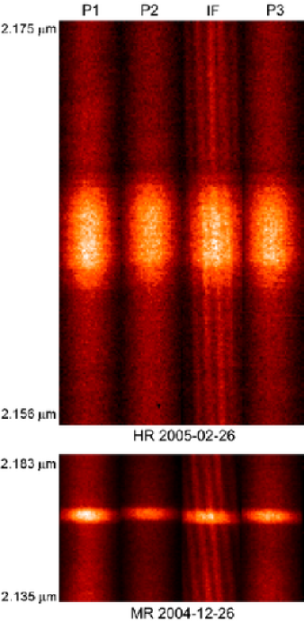
Figure 1: Spectrally dispersed VLTI/AMBER Michelson interferograms of $\eta$ Car. The two panels show the spectrally dispersed fringe signal (IF) as well as the photometric calibration signals from the three telescopes (P1-P3) in high (HR, upper panel) and medium spectral resolution mode (MR, lower panel). In both panels, the bright regions are associated with the Doppler-broadened Br$\gamma$ emission line.

AMBER (Petrov et al., 2003, 2006a, 2006b) is the near-infrared ($J$, $H$, $K$ band) beam-combiner instrument of ESO’s Very Large Telescope Interferometer, which allows the measurement of visibilities, differential visibilities, differential phases, and closure phases (Petrov et al., 2003; Millour et al., 2006). AMBER offers three spectroscopic modes: low (LR mode; R=$\lambda/\Delta\lambda$=75), medium (MR mode; R=1,500), and high (HR mode; R=12,000) spectral resolutions. The fibers in AMBER limit the field-of-view to the diameter of the fibers on the sky ($\sim 60\,$mas). In AMBER the light is spectrally dispersed using a prism or grating. The AMBER detector is a Hawaii array detector with 512$\times$512 pixels.

Figure 1 shows two AMBER raw interferograms taken in the wavelength range around the Br$\gamma$ line in HR (top) and MR (bottom) mode. In the MR data sets, the Doppler-broadened Br$\gamma$ line covers $\sim 8$ spectral channels, whereas in HR mode, the line is resolved by $\sim 50$ spectral channels.

$\eta$ Car was observed with AMBER on 2004 December 26, 2005 February 25, and 2005 February 26 with the three 8.2 m Unit Telescopes UT2, UT3, and UT4. With projected baseline lengths up to 89 m, an angular resolution of $\sim$5 mas was achieved in the $K$ band. As listed in Table 1, the MR-K observations were performed in the wavelength range around both the He I 2.059 $\mu$m and the Br$\gamma$ 2.166 $\mu$m emission lines. The HR-K observations were only performed in a wavelength range around the Br$\gamma$ line. The widths of the wavelength windows of the obtained MR-K and HR-K observations are approximately 0.05 $\mu$m and 0.02 $\mu$m, respectively.

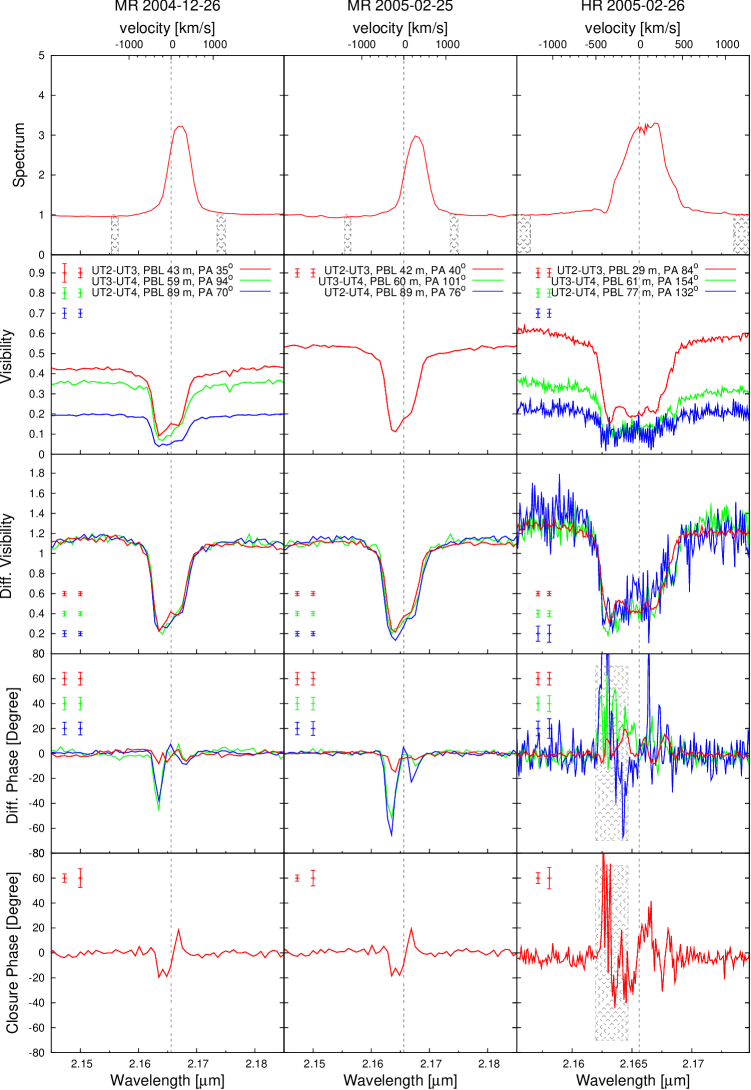
Figure 2: AMBER observables derived from our $\eta$ Car data around the Br$\gamma$ line for three independent measurements (Left: MR, 2004 December 26, Middle: MR, 2005 February 25, Right: HR, 2005 February 26). The first row shows the continuum-normalized spectra as extracted from the interferometric channels, followed by the derived calibrated visibilities and the differential visibilities. In the fourth and fifth row, the differential phase and the closure phase are presented. In the spectra we mark the wavelength regimes, which we defined as continuum for our analysis (shaded regions). The vertical grey line marks the rest-wavelength of Br$\gamma$ ($\lambda_{\rm vac}=2.1661\,\mu$m; the small correction due to the system velocity of -8 km/s (Smith, 2004) has been neglected). We show different error bars within each panel: The left error bars correspond to the total (including statistical and systematic) error estimated for the continuum wavelength range, and the error bar towards the right visualizes the total error for the wavelength range within the line. For the HR 2005-02-26 measurement, data splitting showed that for a small wavelength range (hatched areas in the two lower right panels), the differential phase for the longest and middle baseline as well as the closure phase become very noisy and are therefore not reliable. Furthermore, the HR differential phase of the longest baseline is noisy at all wavelengths. See Sect. 2 for further details.

For the reduction of the AMBER data, we used version 2.4 of the amdlib software package. This software uses the P2VM ( pixel-to-visibilities matrix) algorithm (Tatulli et al., 2006) in order to extract complex visibilities for each baseline and each spectral channel of an AMBER interferogram. From these three complex visibilities, the amplitude and the closure phase are derived. While the closure phase is self-calibrating, the visibilities have to be corrected for atmospheric and instrumental effects. This is done by dividing the $\eta$ Car visibility through the visibility of a calibrator star measured on the same night. In order to take the finite size of the calibrator star into account, the calibrator visibility is corrected beforehand through division by the expected calibrator star visibility (see Table 1). In the case of the MR measurement performed on 2005-02-25, the interferograms recorded on the calibrator contain only fringes corresponding to the shortest baseline (UT2-UT3). Thus, the $\eta$ Car visibility for this night could only be calibrated for this shortest baseline.

Besides the calibrated visibility and the closure phase, the spectral dispersion of AMBER also allows us to compute differential observables; namely the differential visibility and the differential phase (Petrov et al., 2003, 2006a, 2006b; Millour et al., 2006). These quantities are particularly valuable, as they provide a measure of the spatial extent and spatial offset of the line-emitting region with respect to the continuum emission. Since the measured complex visibilities are affected by wavelength-dependent atmospheric piston (optical path difference), the piston has to be estimated and subtracted. This was done using the ammyorick¹ tool (version 0.56).

Since a large fraction of the interferograms is of low contrast (probably due to vibration; see Malbet et al. 2006), we removed a measurement from the data sets if (a) the intensity ratio of two of the photometric channel signals is larger than 4 (a large ratio means that the interferograms are very noisy since the signal is very weak in one channel) or (b) it belongs to the 70 percent of the interferograms with the lowest fringe contrast SNR (with the SNR defined as in Tatulli et al. 2006). In order to optimize the selection for each baseline of the telescope triplet, both of these criteria are applied for each telescope pair individually. Furthermore, the first 10 frames in each new sequence of recorded interferograms are removed since they are degraded by electronic noise.

Figures 2 and 4 show the spectra as well as the wavelength dependence of the visibilities, differential visibilities, differential phases, and closure phases derived from the AMBER interferograms for the observations around the Br$\gamma$ and He I emission lines. The uv coverage of the observations is displayed in Fig. 3.

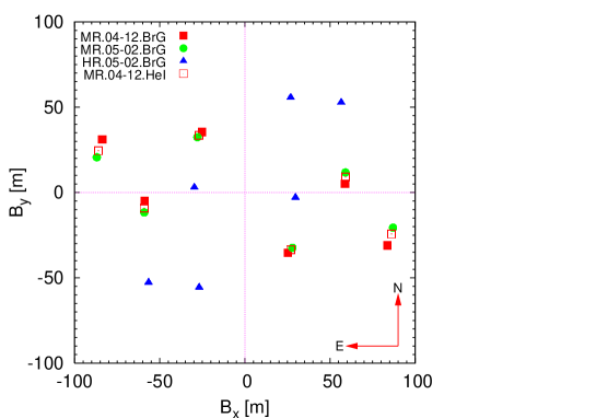
Figure 3: uv coverage of the AMBER $\eta$ Car observations. The data obtained with medium spectral resolution in Dec. 2004 and Feb. 2005 are indicated by red squares and green bullets, respectively, while the high-resolution measurements are shown as blue triangles. Filled symbols denote observations around the Br$\gamma$ line, and open symbols denote observations around the He I line.

The $\eta$ Car spectra were corrected for instrumental effects and atmospheric absorption through division by the calibrator spectrum. For the HR 2005-02-26 measurement, we found that the calibrator itself (L Car) shows prominent Br$\gamma$ line absorption (see Fig. 12). Therefore, we had to remove this stellar line by linear interpolation before the spectrum could be used for the calibration. The wavelength calibration was done using atmospheric features, as described in more detail in Appendix A.

In order to test the reliability of our results, we split each of the raw data sets into 5 subsets, each containing the same number of interferograms. The results obtained with these individual subsets allowed us to test that the major features detected in the visibility, differential visibility, differential phase, and closure phase are stable, even without any frame selection applied. As an exception, we found that for a small wavelength range of the HR 2005-02-26 data set (hatched areas in the two lower right panels of Figure 2), the differential phase corresponding to the middle and longest baselines and the closure phase vary strongly within the subsets and are, therefore, unreliable. This is likely due to the very low visibility value on these two baselines, resulting in a low fringe SNR within this wavelength range. Furthermore, with this method we found that the differential visibility, differential phase, and closure phase extracted from the MR 2005-02-25 He I data set are very noisy and not reliable. Therefore, these differential quantities and closure phases were dropped from our further analysis.

The subsets were also used to compute statistical errors. We estimated the variance for each spectral channel and derived formal statistical errors for both the continuum and line wavelength ranges. In each panel of Figures 2 and 4, we show two types of error bars corresponding to these regions, which not only take these statistical errors but also a systematic error (e.g. resulting from an imperfect calibration) into account.

3 Observational results and interpretation

3.1 Comparison of the observed wavelength dependence of the visibility with the NLTE radiative transfer model of Hillier et al. (2001)

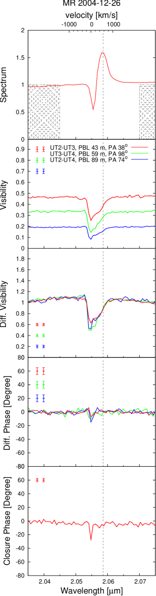
Figure 4: Similar to Fig. 2, but showing the MR measurement from 2004 December 26 covering the region around the He I line. The vertical grey line marks the He I rest-wavelength ($\lambda_{\rm vac}=2.0586\,\mu$m).

For the analysis presented in this chapter, we used the AMBER data sets from 2004 Dec. 26 and 2005 Feb. 25 and 26, presented in Figs. 2 and 4, and compared the AMBER visibilities and spectra with the NLTE radiative transfer model of Hillier et al. (2001). To directly compare the AMBER measurements with this model, we derived monochromatic model visibilities for all wavelengths between 2.03 and 2.18$\,\mu$m (with $\Delta\lambda=10^{-4}\,\mu$m) from the model intensity profiles, assuming a distance of 2.3 kpc for $\eta$ Car. The comparison is visualized in Fig. 5 for the individual AMBER HR and MR measurements. The first row displays the AMBER and model spectra, while all other panels show the AMBER and model visibilities for the different projected baselines. We note that for the comparison shown in Fig. 5, we used the original model of Hillier et al. (2001) without any additional size scaling or addition of a background component.

As the figure reveals, the NLTE model of Hillier et al. (2001) can approximately reproduce the AMBER continuum observations for all wavelengths (i.e. 2.03–2.18$\,\mu$m) and all baselines. Moreover, the wavelength dependence of the model visibilities inside the Br$\gamma$ line is also similar to the AMBER data. There is a slight tendency for the model visibilities in the Br$\gamma$ line to be systematically lower, which can be attributed to the overestimated model flux in the line. On the other hand, there is an obvious difference in the wavelength dependence of the visibility across the He I line between the observations and the model predictions. This difference probably indicates that the primary wind model does not completely describe the physical origin and, hence, the spatial scale of the He I line-forming region. The discrepancy is possibly caused by additional He I emission from the wind-wind interaction zone between the binary components and by the primary’s ionized wind zone caused by the secondary’s UV light illuminating the primary’s wind (e.g., Davidson et al., 1999; Davidson, 2001; Pittard & Corcoran, 2002; Steiner & Damineli, 2004; Hillier et al., 2006; Nielsen et al., 2006; Martin et al., 2006), as discussed in Sects. 1, 3.4.2, and 3.7.2 in more detail.

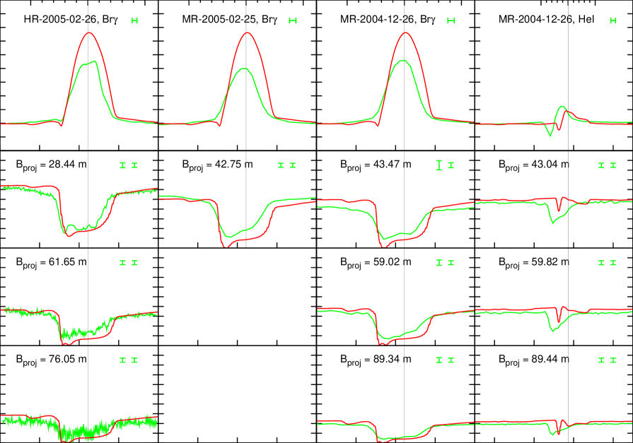
Figure 5: Comparison of the AMBER spectra and visibilities with the NLTE model predictions of Hillier et al. (2001). The figure displays the spectra (upper row) and visibilities (lower three rows, see labels for projected baselines) of the four AMBER measurements (green lines) and the corresponding data of the Hillier et al. NLTE model (red lines). The errors of the AMBER continuum and line visibility measurements are indicated by the two vertical error bars (see Figs. 2 and 4; the left bar is the continuum error bar), and the uncertainty of the AMBER wavelength calibration is indicated by the horizontal error bar. As the figure shows, we find good agreement between the AMBER data and the model predictions for the continuum visibilities as well as the shape and depth of the visibility inside the Br$\gamma$ line. In the case of the He I line, the wavelength dependence of the model visibility inside the line differs considerably from the AMBER measurements, indicating a different physical process involved in the line formation (see Sect. 3.1). The He I wavelength shift can be attributed to a combination of both Doppler shift (e.g. Nielsen et al., 2006; Hillier et al., 2006) and uncertainties in the wavelength calibration of the AMBER data. Note that no additional scaling has been applied to the Hillier et al. model. The model spectra and visibilities have a spectral resolution ($\lambda/\Delta\lambda\sim 20,000$) comparable to the HR measurements.

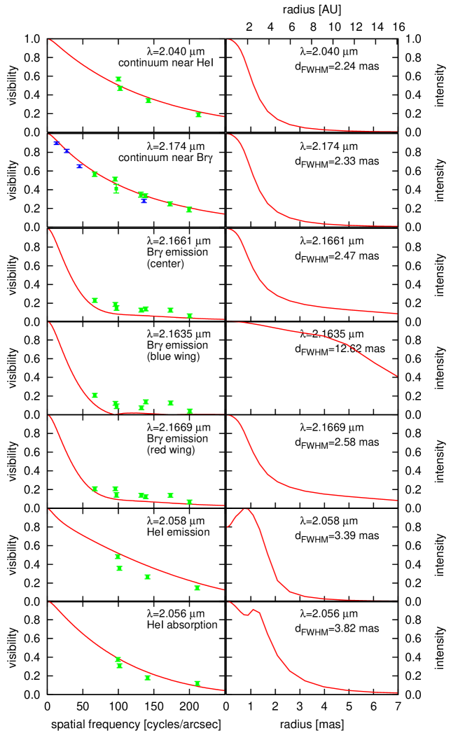
Figure 6: Left: Comparison of the AMBER visibilities (filled green squares; baseline range 28–89 m) as a function of spatial frequency with the NLTE model predictions of Hillier et al. (2001) (solid red lines) for two continuum wavelengths (upper two panels; see labels for the exact wavelengths), the central wavelength of the Br$\gamma$ emission line (third), wavelengths in the blue and red wing of the Br$\gamma$ emission line (fourth and fifth row; at these wavelengths, the AMBER data show the strongest differential and closure phase signals), and the central wavelengths of the He I emission and P Cygni absorption (lower two panels). The blue triangles are the background-corrected VINCI $K$-band measurements from van Boekel et al. (2003). Right: Center-to-limb variation (CLV; i.e. intensity as a function of angular radius) of the monochromatic Hillier et al. (2001) NLTE models for the wavelengths indicated by the labels. As the figures show, the typical FWHM diameter of the models is of the order of $\sim$2–4 mas for an assumed distance of 2.3 kpc for $\eta$ Car. See text for details.

Figure 6 shows the AMBER and model visibilities as a function of spatial frequency and the corresponding model center-to-limb intensity variations (CLVs) for seven selected wavelengths (2 continuum wavelengths; center, blue-shifted, and red-shifted wings of Br$\gamma$ emission; center of both He I emission and absorption). As Fig. 6 reveals, at several wavelengths we find a very good agreement between the visibilities measured with AMBER and the visibilities predicted by the model of Hillier et al. (2001). This is especially true for the continuum data (upper two panels).

¿From the model CLVs, FWHM model continuum diameters of 2.24 mas and 2.33 mas can be derived for $\lambda=2.040$ and 2.174 $\mu$m, respectively. If we allow for a moderate rescaling of the size of the model, we find that the best $\chi^{2}$ fit at both continuum wavelengths can be obtained with scaling factors of 1.015 and 1.00, respectively. This means that the model size has to be increased by only 1.5% at $\lambda=2.040\,\mu$m and that the best fit at 2.174 $\mu$m is indeed obtained with the original Hillier model with a scaling factor of 1.0. Thus, taking the slight rescaling for the best $\chi^{2}$ fit into account, we can conclude that, based on the NLTE model from Hillier et al. (2001, 2006) and the AMBER measurements, the apparent FWHM diameters of $\eta$ Car in the $K$-band continuum at $\lambda=2.040\,\mu$m and 2.174 $\mu$m are 2.27 mas and 2.33 mas, respectively (see Table 2), corresponding to a physical size of approximately 5 AU.

Since the deviations between the model and the measurements are larger in the case of the Br$\gamma$ and He I line data (lower 5 panels in Fig. 6), the scaling factors corresponding to the best $\chi^{2}$ fit in the lines show stronger deviations from unity. For the Br$\gamma$ emission line, we find scaling factors of 0.74, 0.76, and 0.78 for $\lambda=2.1661,2.1635,$ and $2.1669\,\mu$m, corresponding to FWHM diameters of 1.83, 9.52 and 2.02 mas (see Table 2).

For the He I emission line, rescaled models with scaling factors of 1.24 and 1.11 provide the best $\chi^{2}$ fit for the peaks of the emission and absorption within the He I line ($\lambda=2.058$ and $2.056\,\mu$m), resulting in FWHM diameters of 4.24 and 4.19 mas, respectively.

In addition to the inner CLV core, at several wavelengths, the CLVs show a very extended wing corresponding to the extended Br$\gamma$ and He I line emission regions. Since the intensity in the wing is much lower than 50% of the peak intensity, the FWHM diameter is not very sensitive to this part of the CLV. In other words, in the case of CLVs with multiple or very extended components, a FWHM diameter can be quite misleading. In such a case, it seems to be more appropriate to use, for instance, the diameter measured at 10% of the peak intensity ($d_{10\%}$) or the 50% encircled-energy diameter ($d_{\rm 50\%\,EED}$). For example, at $\lambda=2.1661\,\mu$m we obtain $d_{10\%}=9.39$ mas and $d_{\rm 50\%\,EED}=9.58$ mas, while for the continuum at $2.174\,\mu$m we find $d_{10\%}=5.15$ mas and $d_{\rm 50\%\,EED}=4.23$ mas. Thus, based on $d_{\rm 50\%\,EED}$, $\eta$ Car appears $\sim 2.2$ times larger at $\lambda=2.1661\,\mu$m compared to the continuum at $\lambda=2.174\,\mu$m. The best-fit model diameters at the other wavelengths are listed in Table 2. The errors of the diameter measurements are $\pm 4\%$ for the two continuum diameters and $\pm 10\%$ for the line diameters, derived from the visibility errors and the uncertainty of the fitting procedure.

Table 2: Diameters obtained by fitting Hillier et al. (2001) model visibilities to the measured AMBER visibilities. Errors are $\pm 4\%$ for the diameters in the continuum and $\pm 10\%$ in the lines (see text).

Spectral region	Wavelength	$d_{\rm FWHM}$	$d_{\rm 10\%}$	$d_{\rm 50\%\,EED}$
	[$\mu$m]	[mas]	[mas]	[mas]
continuum	2.0400	2.27	4.85	3.74
continuum	2.1740	2.33	5.15	4.23
Br$\gamma$ (center)	2.1661	1.83	9.39	9.58
Br$\gamma$ (blue wing)	2.1635	9.52	16.46	9.60
Br$\gamma$ (red wing)	2.1669	2.02	9.61	9.78
He I (absorption)	2.0560	4.24	8.22	5.36
He I (emission)	2.0580	4.19	4.30	6.53

$d_{\rm FWHM}$ = FWHM diameter; $d_{\rm 10\%}$ = diameter measured at 10% peak intensity; $d_{\rm 50\%\,EED}$ = 50% encircled-energy diameter.

3.2 Continuum visibilities

3.2.1 Comparison of the continuum visibilities with the Hillier et al. (2001) model predictions

The comparison of the AMBER continuum visibilities with the NLTE model from Hillier et al. (2001, 2006) is shown in the two upper left panels of Fig. 6 for the continuum near the He I $2.059\,\mu$m and Br$\gamma$ 2.166$\,\mu$m emission lines (the exact wavelengths are described in Fig. 6). Taking a slight rescaling into account, we concluded in the previous section that, based on the NLTE model from Hillier et al. (2001) and the AMBER measurements, the apparent 50% encircled-energy diameters $d_{\rm 50\%\,EED}$ of $\eta$ Car in the $K$-band continuum at $\lambda=2.040\,\mu$m and 2.174 $\mu$m are 3.74 mas and 4.23 mas, respectively (see Table 2). These diameters are in good agreement with the 50% encircled-energy $K$-band diameter of 5 mas reported by van Boekel et al. (2003).

For comparison, we also fitted the AMBER visibilities with simple analytical models such as Gaussian profiles, as described in more detail in Sect. B in the Appendix. From a Gaussian fit of the AMBER visibilities, we obtain a FWHM diameter of $d_{\rm Gauss}\sim 4.0\pm 0.2\,$mas in the $K$-band continuum. As outlined in Sect. B, the diameter value strongly depends on the range of projected baselines used for the fit, since a Gaussian without an additional background component is not a good representation of the visibility measured with AMBER. As discussed in Appendix B, using a Gaussian fit with a fully resolved background component as a free parameter results in a best fit with a 30% background flux contribution (see also Petrov et al., 2006a).

3.2.2 Comparison of the VINCI and AMBER continuum visibilities

In Fig. 6 (left, second row) displaying the averaged Br$\gamma$ continuum data, the visibilities of $\eta$ Car obtained with VLTI/VINCI are shown in addition to the AMBER data. These VINCI measurements were carried out in 2002 and 2003 using the 35 cm test siderostats at the VLTI with baselines ranging from 8 to 62 m (for details, see van Boekel et al., 2003). Like AMBER, VINCI is a single-mode fiber instrument. Therefore, its field-of-view is approximately equal to the Airy disk of the telescope aperture on the sky, which is $\sim 1.4^{{}^{\prime\prime}}$ in the case of the siderostats. From the VINCI measurements and using only the 24 m baseline data, van Boekel et al. (2003) derived a FWHM Gaussian diameter of $d_{\rm Gauss}\sim$ 7 mas for the wind region of $\eta$ Car. At first glance, this diameter measurement seems to contradict the $d_{\rm Gauss}\sim 4.0$ mas FWHM diameter derived from the AMBER data. This is not the case, however, since the diameter fit is very sensitive to the baseline (or spatial frequency) fit range, because a Gaussian is not a good representation of the visibility curve at all, as can be seen in Fig. 13. If only the VINCI data points are fitted, which have spatial frequencies $<$ 60 cycles/arcsec (corresponding to projected baselines $<$ 28 m), $d_{\rm Gauss}\sim 7$ mas provides the best fit. On the other hand, if the data point at 136 cycles/arcsec (corresponding to a projected baseline of $\sim 62$ m) is included in the fit, we obtain $d_{\rm Gauss}\sim 4.3\,$mas (see also the discussion Sect. B). Thus, when using comparable baseline ranges for the Gaussian fits, there is good agreement between the AMBER and VINCI measurements.

To account for the background contamination of the VINCI data caused by nebulosity within VINCI’s large 1.4${}^{{}^{\prime\prime}}$ field-of-view (in which, for instance, all speckle objects B, C, and D are located), van Boekel et al. introduced a background component (derived from NACO data) providing 55% of the total flux. Adding this background component to the model of Hillier et al. (2001), they found a good match between the model and the observations. Since our AMBER observations were carried out with the 8.2 m Unit Telescopes of the VLTI, the field-of-view of the AMBER observations was only $\sim$60 mas. Thus, the background contamination of the AMBER data can be expected to be much weaker, if not negligible, compared to the VINCI measurements. To check this, we first performed a fit of the Hillier et al. (2001) model, which not only contains the size scaling as a free parameter, but also a fully resolved background component. As we expected, we found the best fit (smallest $\chi^{2}$) with no background contamination. Therefore, when we finally compared the AMBER observations with the model from Hillier et al. (2001), we did not introduce a background component. In Fig. 6 (second row, left) we plot both the AMBER visibilities (no background correction required) plus the background-corrected VINCI data (assuming a 55% background contribution; blue triangles). As can be seen from the figure, these VINCI points nicely match the AMBER data and the corresponding fit of the NLTE model from Hillier et al. (2001). Therefore, from the analysis of the continuum data, we can conclude that the background contamination in the AMBER measurements is negligible and that the AMBER measurements are in good agreement with both the previous VINCI measurements and the model predictions from Hillier et al. (2001).

3.3 Elongated shape of the continuum intensity distribution

To look for detectable elongations of the continuum intensity distribution, we fitted an elliptically stretched 2-D version of the radiative transfer model visibilities from Hillier et al. (2001) to the measured visibilities. Our best $\chi^{2}$ fit reveals a projected axis ratio of $\xi\,=\,1.18\pm 0.10$ and PA $=\,120\pm 15$°. Comparison with the results found by van Boekel et al. (2003) shows that the projected axis ratio $\xi$ derived from the AMBER data is in basic agreement with the $K$-broad-band values of $\xi\,=\,1.25\pm 0.05$ and PA$\,=\,138\pm 7\degr$ from van Boekel et al. (2003).

We also studied the elongation inside the Br$\gamma$ emission line at $\lambda=2.166\,\mu$m, following the same procedure as in the continuum; i.e., we fitted an elliptically stretched 2-D version of the Hillier et al. model shown in Fig. 6 to the AMBER data. However, since the global shape of the model function at $\lambda=2.166\,\mu$m shows stronger deviations from the measurements than in the continuum, the elongation determination suffers from larger uncertainties, resulting in large error bars of the fit parameters. For instance, for $\lambda=2.166\,\mu$m we obtained $\xi=1.66\pm 0.60$ and PA=81$\pm 40$°  from the best ellipse fit.

The 2-D ellipse fitting was also performed for the continuum near the He I emission line and in the center of the He I line ($\lambda=2.057\,\mu$m), where our model fits give an axis ratio of $\xi=1.35\pm 0.30$ and a PA of the major axis of $98\pm 40\degr$ in the continuum, and $\xi=1.74\pm 0.60$ and PA = $159\pm 40\degr$ in the center of the He I emission line. It should be noted that for the He I line region, only four visibility points are available, covering the small PA range of only $60\degr$. Because of this limited number of data points and the small PA coverage, we conclude that the He I elongation measurements in the continuum as well as the line region are not reliable and abandoned in the further elongation analysis of the He I data.

¿From the K-band VINCI data, van Boekel et al. (2003) derived a PA of $138\pm 7\degr$ for the major axis, very well aligned with the Homunculus ($132\degr$, Davidson et al., 2001) and in agreement with our results (PA $=120\pm 15$°). Van Boekel’s and our continuum elongation measurements favor the physical model according to which $\eta$ Car exhibits an enhanced mass loss in polar direction as proposed, for instance, by Owocki et al. (1996, 1998) or Maeder & Desjacques (2001) for stars rotating close to their critical rotation speed. Axis ratios of the order of 1.2 appear reasonable in the context of such polar-wind models. Suppose, for example, that the wind’s polar/equatorial density ratio is 2 at any given radius $r$, as reported by Smith et al. (2003) to explain latitude-dependent changes in the Balmer line profiles. Relevant absorption and scattering coefficients have radial dependencies between $n_{e}\sim r^{-2}$ (Thomson scattering) and $n_{e}^{2}\sim r^{-4}$ (most forms of thermal absorption and emission). A meridional map of projected optical thickness through the wind would show cross-sections of prolate spheroids, correlated with the appearance of the configuration. With the radial dependencies and polar/equatorial density ratio mentioned above, these spheroids have axial ratios between about 1.2 and 1.4; i.e., appreciably less than 2. Viewed from an inclination angle $i\approx 45$°(Davidson et al., 2001), the apparent (projected) axis ratios are between 1.1 and 1.2. This is merely one example, and we have omitted many details, but it illustrates that the polar/equatorial density ratio is around 2, in agreement with Smith et al. (2003).

Finally, Smith et al. (2003) suggested that the stellar wind should become basically spherical during an event at periastron. This prediction can be tested if VLTI/AMBER data are obtained at the next periastron passage.

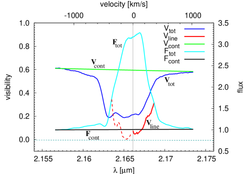
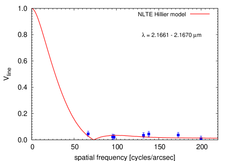
Figure 7: Top: The solid and dashed red lines show the continuum-corrected visibility inside the Br$\gamma$ line of the HR measurement with the shortest projected baseline (29 m). The continuum correction follows Eq. (2). Except for the phase, all quantities entering Eq. (2) are indicated in the figure. We assume $F_{\rm tot}=F_{\rm cont}+F_{\rm line}$ and that $F_{\rm cont}$ inside the line is approximately equal to the level outside the line. The continuum-corrected visibility in the blue-shifted region of the emission line is shown with a dashed line since it is highly uncertain due to the presence of the P Cygni-like absorption component (see text for details). Bottom: Continuum-corrected AMBER visibilities (filled blue squares) in the red region of the Br$\gamma$ line as a function of spatial frequency. To derive the visibilities according to Eq. (2), the data in the wavelength range 2.1661–2.1670$\,\mu$m (red-shifted line region) were averaged before the continuum correction. The solid red line shows the continuum-corrected model visibility. Obviously, observations at shorter baselines are needed to further test the model predictions.

3.4 Continuum-corrected visibilities

3.4.1 Continuum-corrected visibility in the Br$\gamma\,$emission line

To investigate the brightness distribution in the Br$\gamma$ line in more detail, we tried to disentangle the continuum and pure line emission from both the AMBER data as well as the model data to derive the size of the pure Br$\gamma$ line-emitting region. Since the visibility measured inside an emission or absorption line is the composite of a pure line component and an underlying continuum, the measured line visibility, $V_{\rm tot}$ (see Fig. 7 top), has to be corrected for the continuum contribution to obtain the visibility $V_{\rm line}$ of the line emitting (absorbing) region. As discussed in Malbet et al. (2006), $V_{\rm line}$ can be calculated if the continuum level within the line is known. If the continuum within the line is equal to the continuum level outside the line for an optically thin environment, as assumed in Fig. 7, we obtain:

$$V_{\rm line}=\frac{V_{\rm tot}\cdot F_{\rm tot}-V_{\rm cont}\cdot F_{\rm cont}}{F_{\rm line}}$$ (1)

with $F_{\rm tot}=F_{\rm cont}+F_{\rm line}$ being the total measured flux and $V_{\rm tot}$ being the measured visibility (also see Fig. 7 top for illustration). As outlined in the Appendix, taking a non-zero differential phase $\Phi^{\prime}$ into account introduces an additional term in Eq. (1), leading to

$$V_{\rm line}=\frac{\sqrt{|V_{\rm tot}F_{\rm tot}|^{2}+|V_{\rm cont}F_{\rm cont}|^{2}-2V_{\rm tot}F_{\rm tot}V_{\rm cont}F_{\rm cont}\cdot\cos\Phi^{\prime}}}{F_{\rm line}}$$ (2)

We applied Eq. (2) to the line-dominated AMBER data in the 2.155-2.175$\,\mu$m Br$\gamma$ wavelength range to derive the continuum-corrected visibility of the region emitting the Br$\gamma$ line radiation. One big uncertainty in this correction is the unknown continuum flux within the line. Due to intrinsic absorption, the continuum flux might be considerably lower within the line than measured at wavelengths outside the line. Especially the blue-shifted wing of the Br$\gamma$ emission line might be affected by the P Cygni-like absorption, as discussed below. In case such an absorption component is present, our continuum-correction would overestimate the size of the line-emitting region. The influence of this effect on the red-shifted wing of the line is likely to be much smaller, as P Cygni-like absorption mainly affects the blue-shifted emission.

The visibility across the Br$\gamma$ line is shown in Fig. 7 (top) for the HR data corresponding to the shortest projected baseline. The results for the other data sets are similar. ¿From Fig. 7 (top), one can see that after the subtraction of a continuum contribution equal to the continuum outside the line, the visibility reaches very small values in the center of the emission line. This means that the pure line-emitting region is much larger than the region providing the continuum flux.

Fig. 7 (top) shows a strong asymmetry between the blue- and red-shifted part of the visibility in the line with respect to the spectrum. While the visibility ($V_{\rm tot}$ as well as $V_{\rm line}$) rises concomitantly with the drop of the line flux on the red side, the situation is very different on the blue side line center. In agreement with the model predictions from Hillier et al. (2001), this indicates the existence of a P Cygni-like absorption component in this wavelength region. In fact, at $\lambda=2.1625\,\mu$m, we see a small dip in the Br$\gamma$ spectrum in both the model spectrum from Hillier et al. (2001) and the HR AMBER observations. If such an absorption component is present, it can explain the asymmetric behaviour of the line visibility with respect to the spectrum. The P Cygni absorption in the blue wing of the Br$\gamma$ line makes the continuum correction of the visibility uncertain for wavelengths shorter than the central wavelength $\lambda_{\rm c}$ of the emission line. Because of this uncertainty, in Fig. 7 (top) the continuum corrected visibility is shown with a dashed line for $\lambda<\lambda_{\rm c}$, and the following discussion is restricted to the red-shifted region of the Br$\gamma$ line emission.

The continuum-corrected AMBER visibilities in the red-shifted region of the Br$\gamma$ line are displayed in Fig. 7 (bottom) for all data sets. To derive the visibilities in the red region, the data in the wavelength range 2.1661–2.1670$\,\mu$m were averaged before the continuum correction. To now compare the continuum-corrected AMBER visibilities with the model predictions (2.1661–$2.1670\,\mu$m), we constructed a model intensity profile of the pure Br$\gamma$ emission line region by subtracting the Hillier et al.  intensity profile of the nearby continuum from the combined line + continuum profile.

As Fig. 7 illustrates, the model prediction is in agreement with the low visibilities found for spatial frequencies beyond 60 cycles/arcsec. On the other hand, the figure also clearly indicates that measurements at smaller projected baselines are needed to further constrain the Hillier et al. model in the line-emitting region. With the baseline coverage provided by the current AMBER measurements, we obtain a FWHM diameter of $\gtrsim 15.4$ mas (lower limit) for the (continuum-corrected) line-emitting region in the red line wing.

3.4.2 Continuum-corrected visibility in the He I emission line

As can be seen in Fig. 4, the AMBER spectrum of the He I line shows a P Cygni-like profile with a prominent absorption and emission component. This is in agreement with earlier findings by Smith (2002) from long-slit spectroscopy using OSIRIS on the CTIO 4m telescope.

To estimate the spatial scale of the region emitting the He I emission line, we followed the same approach as outlined in the previous section for the Br$\gamma$ line; i.e., we first applied Eq. (2) and then compared the continuum-corrected visibility with the continuum-corrected radiative transfer model of Hillier et al. (2001). Figure 8 (top) shows the measured flux and visibility for the MR-2004-12-26 measurement with the shortest projected baseline (43m) as well as the continuum-corrected visibility across the He I emission component (solid red line). Because of the P Cygni-like absorption component, the continuum subtraction is highly uncertain in the blue region of the emission line (dashed red line in Fig. 8), as already discussed in the context of the Br$\gamma$ line in Sect. 3.4.1.

In Fig. 8 (bottom), the continuum-corrected visibility of all AMBER data in the red region of the He I emission line (averaged over the wavelength range 2.057–2.058$\,\mu$m) is shown as a function of spatial frequency. As the figure reveals, similar to the Br$\gamma$ emission, the visibilities inside the He I emission line region reach rather low values. As the comparison shows, the line visibilities predicted by the model are much higher than the line visibilities measured with AMBER, indicating that the size of the line-emitting region in the model is too small. Rescaling of the model size by a factor of 2.4 results in a much better agreement between the model and observations (green curve in Fig. 8, bottom) and a FWHM diameter of $\gtrsim 8.2$ mas, which is 3.6 times larger than the FWHM diameter of 2.3 mas in the continuum. Due to the lack of interferometric data at small projected baselines, this value can only give a rough lower limit of the size.

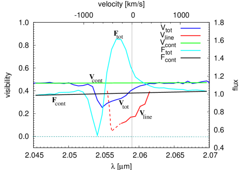
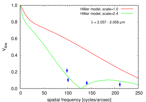
Figure 8: Visibility in the He I line. Top: The figure is similar to Fig. 7 (top) but displays the MR-2004-12-26 data with the shortest projected baseline (43m). As in the case of the Br$\gamma$ emission, the figure reveals that the region dominated by line emission is fully resolved by the AMBER measurements. As in Fig. 7 (top), the continuum-corrected visibility is shown with a dashed line in the blue-shifted region of the emission line to indicate that in this region, the line visibility is highly uncertain due to the presence of the P Cygni absorption. Bottom: Continuum-corrected AMBER visibilities (filled blue squares) in the red region of the He I emission line as a function of spatial frequency and continuum-corrected visibility curve (solid red line) according to the NLTE model of Hillier et al. (2001). To derive the visibilities according to Eq. (2), the data in the wavelength range 2.057–2.058$\,\mu$m were averaged before the continuum correction. The model curve predicts much larger visibility values in the line, which indicates that the size of the line-emitting region in the model is probably underestimated by the model. A rescaling of the size of the model by a factor of $\sim$2.3 (green line) reveals better agreement with the AMBER measurements.

The results for the visibility inside the He I line can possibly be explained in a qualitative way in the framework of the binary model for the central object in $\eta$ Car (e.g. Davidson et al., 1999; Davidson, 2001; Pittard & Corcoran, 2002; Hillier et al., 2006; Nielsen et al., 2006). In a model of this type, He I emission should arise near the wind-wind interaction zone between the binary components. The hot secondary star is expected to ionize helium in a zone in the dense primary wind, adjoining the wind-wind interaction region. Such a region can produce He I recombination emission. The wind-wind shocked gas, by contrast, is too hot for this purpose, while the density of the fast secondary wind is too low. Since the AMBER measurements (Dec. 2004 and Feb. 2005, at orbital phases $\phi=0.268$ and $\phi=0.299$, see Table 1) were obtained at an intermediate phase between periastron in July 2003 and apoastron in April 2006, the extension of the He I emission zone is expected to be rather diffuse and larger than the continuum size. In other words, the He I emission zone should be fairly extended and larger than the Hillier et al. model prediction, which is in agreement with the AMBER data.

3.5 Differential Phases and Closure Phases

The measurement of phase information is essential for the reconstruction of images from interferometric data, but such an image reconstruction is only possible with an appropriate coverage of the uv plane. Nevertheless, even single phase measurements, in particular of the closure phase and differential phase, provide important information.

The closure phase (CP) is an excellent measure for asymmetries in the object brightness distribution. In our AMBER measurements, as illustrated in Figs. 2 and 4, we find that the CP in the continuum is zero within the errors for all the various projected baselines of the UT2-UT3-UT4 baseline triplet, indicating a point-symmetric continuum object. However, in the line emission, we detect a non-zero CP signal in all data sets. In both MR measurements covering the Br$\gamma$ line, we find the strongest CP signal in the blue wing of the emission line at $\lambda=2.164\,\mu$m (-34° and -20°) and a slightly weaker CP signal in the red wing of the emission line at $\lambda=2.167\,\mu$m (+12° and +18°). We also detected non-zero CP signals in the HR measurement around Br$\gamma$ taken at a different epoch. In the case of the He I line, a non-zero CP could only be detected at $\lambda=2.055\,\mu$m, just in the middle between the emission and absorption part of the P Cygni line profile.

The differential phase (DP) at a certain wavelength bin is measured relative to the phase at all wavelength bins. Therefore, the DP measured within a wavelength bin containing line emission yields approximately the Fourier phase of the combined object (continuum plus line emission) measured relative to the continuum. This Fourier phase might contain contributions from both the object phase of the combined object and a shift phase, which corresponds to the shift of the photocenter of the combined object relative to the photocenter of the continuum object. Significant non-zero DPs were detected in the Doppler-broadened line wings of the Br$\gamma$ line. Particularly within the blue-shifted wings, we found a strong signal (up to $\sim-60$°), whereas the signals are much weaker within the red-shifted line wings. These DPs might correspond to small photocenter shifts, possibly arising if the outer Br$\gamma$ wind region consists of many clumps which are distributed asymmetrically. The small differential phases of up to $\sim-15$° for the different baselines of the blue-shifted light in the He I line can perhaps also be explained by the above-mentioned asymmetries or within the framework of the binary model discussed in previous sections. In the binary model, a large fraction of the He I is possibly emitted from the wind-wind collision zone, which is located between the primary and the secondary (Davidson et al., 1999; Davidson, 2001; Pittard & Corcoran, 2002; Hillier et al., 2006; Nielsen et al., 2006).

3.6 Modeling with an inclined aspherical wind geometry

The goal of the modeling presented in this section is to find a model which is able to explain several remarkable features in our data; in particular, (a) the asymmetry in the Br$\gamma$ line profile (showing less emission in the blue-shifted wing than in the red-shifted wing) and the P Cygni-like absorption dip in the blue-shifted Br$\gamma$ wing, (b) the strong DP in the blue-shifted wing and a weaker DP signal in the red-shifted wing, and (c) the structure of the CP, showing a change in the sign between the blue- and red-shifted line wing. We aimed for a geometrical but physically motivated model which would reproduce these features at all wavelength channels simultaneously. For this, we concentrate on the Br$\gamma$ line, as this line shows a stronger phase signal than the He I line and was measured with a better uv coverage.

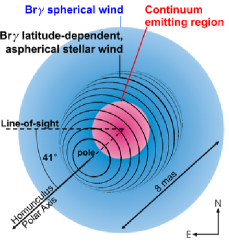
Figure 9: Left: Illustration of the components of our geometric model for an optically thick, latitude-dependent wind (see text for details). For the weak aspherical wind component, we draw the lines of latitudes to illustrate the 3D-orientation of the ellipsoid. Right (a, b): The upper row shows the brightness distribution of the modeled aspherical wind component (item (3) in the text) for two representative wavelengths. The figures below show the total brightness distribution after adding the contributions from the two spherical consituents of our model.

$\begin{array}[]{c @{\hspace{-16mm}} c}\textnormal{{a) Blue-shifted line wing}}&\textnormal{{b) Red-shifted line wing}}\\ \lambda=2.1635\,\mu\textnormal{m}&\lambda=2.1669\,\mu\textnormal{m}\\[-34.1433pt] \includegraphics[width=213.39566pt,angle={0}]{5577f9r1.ps}&\includegraphics[width=213.39566pt,angle={0}]{5577f9r2.ps}\\[-56.9055pt] \includegraphics[width=213.39566pt,angle={0}]{5577f9r3.ps}&\includegraphics[width=213.39566pt,angle={0}]{5577f9r4.ps}\\[-17.07164pt] \end{array}$

As Smith et al. (2003) convincingly showed, the stellar wind from $\eta$ Car seems to be strongly latitude-dependent, with the highest mass flux and velocities at the poles. This anisotropy can be understood in the context of theoretical models (see, e.g., Maeder & Desjacques, 2001), which take the higher temperatures at the poles ($g_{\textnormal{eff}}$-effect) and the equatorial gravity darkening on a rapidly rotating star into account (von Zeipel effect, Zeipel, 1925). As these models are quite successful in explaining the bipolar structure of the Homunculus nebula, we investigated whether such bipolar geometries with a latitude-dependent velocity distribution might also be suited to explain our interferometric data.

Due to its success in reproducing both the spectrum and the measured visibilities, we based our wind model on the spherical Hillier et al. (2001) model and superposed a weak aspherical stellar wind geometry, which is inclined with respect to the line-of-sight. Our model includes three components (see Fig. 9); namely,

(1)

a continuum component (using the Hillier et al. continuum CLV, see Fig. 6 top) with a blue-shifted absorption component,

(2)

a spherical stellar wind (using the Hillier et al. continuum-subtracted Br$\gamma$ CLV), and

(3)

an aspherical wind geometry, represented by a 41° inclined ellipsoid.

The relative contribution of these different constituents to the total flux is given by the input spectra shown in the upper row of Fig. 10. For the spherical and aspherical wind component, we assume Gaussian-shaped spectra. The original Hillier et al. CLVs slightly underestimate the size of the observed structures (see Fig. 5). Therefore, we rescaled them by 10% to obtain a better agreement for the visibilities at continuum wavelengths.

The aspherical wind of $\eta$ Car is simulated as an ellipsoid with an inclination similar to the inclination angle of the Homunculus (41°, Smith, 2006). While the south-eastern pole (which is inclined towards the observer) is in sight, the north-western pole is obscured. The latitude-dependent velocity distribution expected for the $\eta$ Car wind was included in our model by coupling the latitude-dependent brightness distribution of the ellipsoid to the wind velocity. At the highest blue-shifted velocities, mainly the south-eastern polar region contributes to the emission (see Fig. 9a). In the red-shifted line wing, mainly the (obscured) north-western pole radiates (see Fig. 9b). The axis of the ellipsoid was assumed to be oriented along the Homunculus polar axis (PA 132°, Smith 2006) and its axis ratio was fixed to 1.5.

As our simulations show, such an asymmetric geometry can already explain the measured DPs and CPs with a rather small contribution of the asymmetric structure to the total flux (see black line in Fig. 10, upper row). Although the large number of free parameters prevented us from scanning the whole parameter space, we found reasonable agreement with a size of the ellipsoid major axis of 8 mas. Fig. 10 shows the spectrum, visibilities, DPs, and CPs computed from the model.

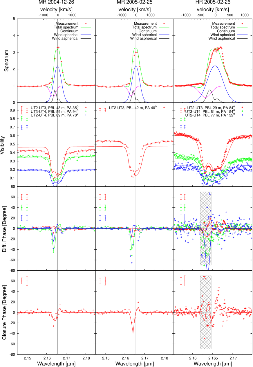
Figure 10: Observables computed from our optically thick, latitude-dependent wind model (see Fig. 9 for a model illustration). The points (crosses) represent the measurements (as also shown in Fig. 2), and the solid lines give the observables computed from our model. The upper row shows the contributions from the various model components to the total flux. Besides the continuum emission (purple line), we introduced a spherical (blue line) and an aspherical (black line) wind component.

As our model was inspired by physical models, but does not take the complicated radiation transport and hydrodynamics involved in reality into account, we would like to note that our model allows us to check for consistency between the considered geometry and the AMBER spectro-interferometric data, but can neither constrain the precise parameters of a possible aspherical latitude-dependent stellar wind around $\eta$ Car, nor can it rule out other geometries. We summarize some qualitative properties of our wind model as follows:

• The strong underlying spherical component mainly accounts for the very low visibilities measured within the line.

• The aspherical wind component introduces the asymmetry required to roughly explain the measured phase signals. In particular, it reproduces the larger DPs and CPs within the blue-shifted line wing compared to the red-shifted wing, as the red-shifted emission region is considerably obscured. It also accounts for the flip in the CP sign, as the photocenter of the line emission shifts its location between the blue- and red-shifted wing relative to the continuum photocenter.

• The absorption component which we introduced in the blue-shifted wing of the Br$\gamma$ line allows us to reproduce the asymmetry measured in the shape of the Br$\gamma$ emission line profile (showing an increase of flux towards red-shifted wavelengths) and the weak dip observed at far-blue-shifted wavelengths. Furthermore, with the decrease of the continuum contribution, the absorption component helps to lower the visibilities in the blue-shifted line wing, simultaneously increasing the asymmetry in the brightness distribution (increasing the phase signals). Finally, with the interplay between the absorption and emission component, our simulation reproduced a ”bump” in the visibility similar to the one observed on the shortest baseline of our HR measurement ($\lambda\approx 2.163\mu$m).

3.7 Feasibility of the detection of the hypothetical hot companion and the wind-wind interaction zone

$\begin{array}[]{ccc}\begin{minipage}[l]{184.9429pt} $\begin{array}[]{c}\textnormal{{a) Continuum emission with binary}}\\[-22.76219pt] \includegraphics[width=156.49014pt,angle={-0}]{5577f11b.ps}\\[-5.69054pt] \textnormal{{b) 2D-Visibility without binary}}\\[-22.76219pt] \includegraphics[width=156.49014pt,angle={0}]{5577f11c.ps}\\[-5.69054pt] \textnormal{{c) 2D-Visibility with binary}}\\[-22.76219pt] \includegraphics[width=156.49014pt,angle={0}]{5577f11d.ps}\end{array}$ \end{minipage}&\begin{minipage}[l]{312.9803pt} $\begin{array}[]{c}\textnormal{{d) Residuals between models with/without a binary}}\\[14.22636pt] \includegraphics[width=312.9803pt,angle={0}]{5577f11a.eps}\end{array}$ \end{minipage}&\end{array}$

Figure 11: Simulation illustrating the signatures of a binary companion at the predicted position (for the orbital phase at the time of our continuum observations around the Br$\gamma$ line; separation $\sim 8$ mas, $PA\sim-36\degr$; see Nielsen et al., 2006). For the primary component, we assume a continuum emission CLV from Hillier et al. (2006), to which we add a uniform disk of 0.1 mas diameter to account for the binary companion (see a). Figure b shows the 2D-visibility function of a single component model containing only the continuum-emitting object with Hillier-type CLV. Figure c shows the 2D-visibility corresponding to the binary model shown in panel a for a small $K$-band flux ratio $q=10$ between the continuum emitting region (Hillier-type CLV) and the companion. In d the residuals of the visibilities (upper panel) and closure phases (lower panel) between the models with and without a companion are shown as a function of flux ratio $q$ for baselines and PAs corresponding to the seven AMBER measurements. The dashed horizontal lines indicate the uncertainty of the measurements. Given these uncertainties, the figure illustrates that a companion signature should be visibile from the AMBER closure phase measurements, if the binary is less than $\sim 110$ times fainter compared to the primary. See text for details.

One of the most intriguing questions regarding $\eta$ Car is whether or not its central object is a binary, as suggested to explain cycle (e.g., Damineli, 1996).

3.7.1 A simple binary continuum model

To investigate whether the AMBER measurements presented here can shed more light on the binarity hypothesis, we used the following approach: We constructed a simple binary model consisting of a primary wind component with a CLV according to the continuum model of Hillier et al. (2006; FWHM diameter $\sim 2.3\,$mas; see upper panels in Fig. 6) and an unresolved binary companion represented by a point-like source (uniform disk with $\sim 0.1$ mas FWHM diameter). The secondary component is predicted to be approximately located at PA –36° with a separation of 8 mas from the primary for the time of the AMBER observations (Nielsen et al., 2006). The continuum flux ratio $q$ was treated as a free parameter. We would like to note that in our model, we assumed that all $K$-band light from the secondary is reaching us unprocessed; i.e. we ignored a possible dilution or re-distribution of the secondary’s radiation.

We calculated the 2D visibility function (see Fig. 11c) of this model intensity distribution for different values of $q$, as well as the closure phases for the baselines and PAs corresponding to our AMBER measurements (Fig. 11d). Finally, we compared the results with those obtained from a single component model where only the primary wind is present (Fig. 11b). The differences of the visibilities and closure phases between the single star and the binary model (at the baselines and PAs corresponding to our AMBER measurements) are displayed in Fig. 11d as a function of the $K$-band flux ratio of the binary components.

Fig. 11d shows two interesting results: First, the closure phase is more sensitive to the binary signature than the visibilities and, thus, a more suitable observable to constrain the binary hypothesis. And second, given the accuracies of our first AMBER visibility and closure phase measurements (indicated by the horizontal dashed-dotted lines), we can conclude, for the particular model shown in Fig. 11, that the AMBER closure phases put an intensity ratio limit $q_{\rm min}\approx 110$ on the binary $K$-band flux ratio. This limit is in line with the estimate $q\approx 200$ given by Hillier et al. (2006). Thus, based on the model shown in Fig. 11, the AMBER measurements are not in conflict with recent model predictions for the binary.

To investigate whether we can put similar constraints on the minimum $K$-band flux ratio $q_{\rm min}$ for arbitrary separations and PAs, we calculated a larger grid of binary models and compared the residuals of visibilities and closure phases analogue to the example shown in Fig. 11.

For these grid calculations, we used values in the range from 4 to 14 mas for the binary separation with increments of 1 mas, and PAs of the secondary in the whole range from 0°  to 360°  in steps of 10°. The $K$-band flux ratio $q$ of the binary components was varied in the range from 1 to 250 with $\Delta q=4$. As a result of the grid calculation, we obtained the minimum $K$-band flux ratio $q_{\rm min}$ as a function of binary separation and orientation.

Whereas the study with a fixed companion position presented above allowed us to put rather stringent constraints on $q_{\rm min}$ (see Fig. 11), this systematic study revealed that due to the rather poor uv coverage, a few very specific binary parameter sets exist where we are only sensitive to $q_{\rm min}\approx 10$. Nevertheless, for the above-mentioned separation interval (4 to 14 mas), we found that we are able to detect companions up to $q_{\rm min}=50$ at more than 90% of all PAs. In order to push this sensitivity limit in future observations, a better uv coverage will be required. Together with the expected higher closure phase accuracy, AMBER will be sensitive up to $q>200$ and, therefore, have the potential to probe the currently favored binary models.

3.7.2 Can AMBER detect a He I wind-wind interaction zone shifted a few mas from the primary wind?

In the context of the binary hypothesis, it is also important to discuss the implications for the interpretation of the AMBER He I measurements. According to the binary model, a large fraction of the He I line emission should arise from the wind-wind collision zone expected between the primary and the secondary (Davidson et al., 1999; Davidson, 2001; Hillier et al., 2006; Nielsen et al., 2006). The exact intensity ratio of primary He I wind and He I emission from the wind-wind interaction zone is not known. Figure  5 suggests that during the AMBER observations, the total He I flux was roughly two times larger than the model prediction of Hillier et al. (2001) for the primary He I wind.

At the orbital phases of the AMBER measurements, the wind-wind collision zone should be at resolvable distances from $\eta$ Car’s primary (resolution $\sim 5\,$ mas; companion separation $\sim 8\,$mas, PA $\sim$ –36°, Nielsen et al., 2006). Looking at the AMBER He I data, we see that the differential as well as the closure phases are zero everywhere except for the transition region between the absorption and emission part of the He I line, where we find differential phases of $\sim 10$–20°  and a closure phase of $\sim$ –30°; i.e., the phases measured across the He I line are significantly weaker compared to the Br$\gamma$ line. The question is now, why AMBER measured weaker phase signals within the He I line and if this result is in line with the predictions of the wind-wind collision model.

One possible explanation for the small measured phases could be the orientation of the binary orbit. If the orbit’s major axis is nearly aligned with the line-of-sight, the photocenter shift inside the He I line will be very small. In addition, the deviations from point symmetry would be rather small. Therefore, in the case of this special geometry, both differential phases and the closure phase would be small, in qualitative agreement with the AMBER data. Another explanation could be that the contribution of the wind-wind collision zone to the He I line emission is much weaker than that of the primary wind. However, this is not very likely (see Hillier et al., 2006).

A different explanation for the weak phases can be found from a modeling approach similar to the one for the Br$\gamma$ line region outlined in Sect. 3.6. Based on the results presented in Sects. 3.1 and 3.4.2, we constructed a simple He I model consisting of a spherical primary wind component with a Hillier-type CLV (2.5 mas FWHM diameter) and an extended spherical He I line-emitting region with Gaussian CLV and a 7 mas FWHM diameter (i.e., for simplicity, we assumed that all He I flux is emitted from the wind-wind interaction region; however, some fraction of He I is also emitted from the primary wind; see Hillier et al. 2006 and Fig. 5 of the present paper). The center of the line-emitting component of this model is located 3 mas away from the primary wind component towards PA 132°; i.e., in the direction of the Homunculus axis. The spectra of the continuum and line-emitting components were chosen in such a way that the combined spectrum resembles the observed He I line spectrum.

The modeling results show that this simple model is approximately able to simultaneously reproduce the observed spectrum and the wavelength dependence of visibilities, differential phases (10–20°), and closure phases ($\sim$ –30°). Thus, our simple model example illustrates that the AMBER measurements can be understood in the context of a binary model for $\eta$ Car and the predicted He I wind-wind collision scenario (e.g. Davidson et al., 1999; Davidson, 2001; Hillier et al., 2006; Nielsen et al., 2006). We note that the model parameter values given above are of preliminary nature. A more detailed, quantitative modeling is in preparation and will be subject of a forthcoming paper. Furthermore, we would like to emphasize, as already discussed in previous sections, that there are likely to be three sources of He I emission - the primary wind, a wind-wind interaction zone (bow shock), and the ionized wind zone caused by the ionization of the secondary. For both the bow shock and the ionized wind zone, the ionizing UV radiation field of the secondary is of crucial importance. On the basis of the observed blue-shift and the weakness of the He I during the event, we believe that the primary wind contribution is small. It is not yet possible to decide on the relative contributions of the bow shock and the ionized wind region.

4 Conclusions

In this paper we present the first near-infrared spectro-interferometry of the enigmatic Luminous Blue Variable $\eta$ Car obtained with AMBER, the 3-telescope beam combiner of ESO’s VLTI. In total, three measurements with spectral resolutions of $R=1,500$ and $R=12,000$ were carried out in Dec. 2004 ($\phi=0.268$) and Feb. 2005 ($\phi=0.299$), covering two spectral windows around the He I and Br$\gamma$ emission lines at $\lambda=2.059$ and $2.166\,\mu$m, respectively. From the measurements, we obtained spectra, visibilities, differential visibilities, differential phases, and closure phases. From the analysis of the data, we derived the following conclusions:

• In the $K$-band continuum, we resolved $\eta$ Car’s optically thick wind. From a Gaussian fit of the $K$-band continuum visibilities in the projected baseline range from 28–89 m, we obtained a FWHM diameter of $4.0\pm 0.2$ mas. Taking the different fields-of-view into account, we found good agreement between the AMBER measurements and previous VLTI/VINCI observations of $\eta$ Car presented by van Boekel et al. (2003).

• When comparing the AMBER continuum visibilities with the NLTE radiative transfer model from Hillier et al. (2001), we find very good agreement between the model and observations. The best fit was obtained with a slightly rescaled version of the original Hillier et al. model (rescaling by 1–2%), corresponding to FWHM diameters of 2.27 mas at $\lambda=2.040\,\mu$m and 2.33 mas at $\lambda=2.174\,\mu$m.

• If we fit Hillier et al. (2001) model visibilities to the observed AMBER visibilities, we obtain, for example, 50% encircled-energy diameters of 4.2, 6.5, and 9.6 mas in the 2.17$\,\mu$m continuum, the He I, and the Br$\gamma$ emission lines, respectively.

• In the continuum around the Br$\gamma$ line, we found an asymmetry towards position angle PA=$120\degr\pm 15\degr$ with a projected axis ratio of $\xi=1.18\pm 0.10$. This result confirms the earlier finding of van Boekel et al. (2003) using VLTI/VINCI and supports theoretical studies which predict an enhanced mass loss in polar direction for massive stars rotating close to their critical rotation rate (e.g.  Owocki et al., 1996, 1998).

• For both the Br$\gamma$ and the He I emission lines, we measured non-zero differential phases and non-zero closure phases within the emission lines, indicating a complex, asymmetric object structure.

• We presented a physically motivated model which shows that the asymmetries (DPs and CPs) measured within the wings of the Br$\gamma$ line are consistent with the geometry expected for an aspherical, latitude-dependent stellar wind. Additional VLTI/AMBER measurements and radiative transfer modeling will be required to determine the precise parameters of such an inclined aspherical wind.

• Using a simple binary model, we finally looked for a possible binary signature in the AMBER closures phases. For separations in the range from 4 to 14 mas and arbitrary PAs, our simple model reveals a minimum $K$-band flux ratio of $\sim$50 with a 90% likelihood.

Our observations demonstrate the potential of VLTI/AMBER observations to unveil new structures of $\eta$ Car on the scales of milliarcseconds. Repeated observations will allow us to trace changes in observed morphology over $\eta$ Car’s spectroscopic 5.5 yr period, possibly revealing the motion of the wind-wind collision zone as predicted by the $\eta$ Car binary model. Furthermore, future AMBER observations with higher accuracy might be sensitive enough to directly detect the hypothetical hot companion.

Appendix A Wavelength calibration

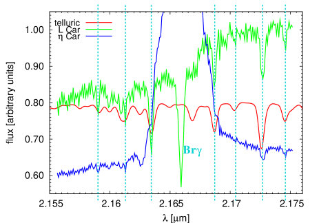
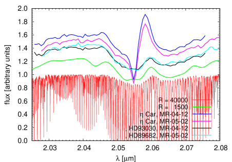
Figure 12: Top: Spectral calibration of the AMBER observations. The figure shows the spectrum of $\eta$ Car (blue) and the calibrator star L Car (green) around the Br$\gamma$ line obtained from the HR measurements in Feb. 2005. In addition, a telluric spectrum from the Kitt Peak Observatory is shown in red. The original telluric spectrum with a spectral resolution of $R=40,000$ was spectrally convolved to match the resolution of the AMBER measurements. For the flux calibration of the $\eta$ Car spectrum, the Br$\gamma$ line in the L Car spectrum was interpolated before the division. See text for further details. Bottom: Same as top panel, but for both MR measurements around the He I emission line. Together with the $\eta$ Car spectra, the spectra of the calibrators HD 93030 and HD 89682 are displayed. In addition, the telluric spectrum obtained at Kitt Peak with $R=40,000$ and a spectrally convolved telluric spectrum is shown, which matches the spectral resolution of the MR measurements ($R=1,500$). The figure illustrates that the forest of telluric lines forms a quasi-continuum which modulates the AMBER spectra.

To obtain both an accurate wavelength calibration of the AMBER raw data and properly calibrated spectra of $\eta$ Car, we compared the AMBER raw spectra of $\eta$ Car as well as the calibrator stars L Car, HD 93030, and HD 89682 with a $K$-band telluric spectrum recorded at the Kitt Peak Observatory with a spectral resolution of 40,000. For the comparison with the AMBER spectrum, this telluric spectrum was spectrally convolved to match the spectral resolution of the AMBER measurements with high ($R\sim 12,000$) and medium ($R\sim 1,500$) spectral resolution.

The result of the comparison is shown in Fig. 12. In the upper panel, the high spectral resolution AMBER spectra of $\eta$ Car and the calibrator L Car are shown together with the telluric spectrum with $R=10,000$. ¿From the comparison with the telluric spectrum, we identified 7 prominent telluric absorption features in the L Car spectrum, which are indicated by the dashed vertical lines. The strongest absorption line seen in the L Car spectrum is not telluric, but can be identified as intrinsic Br$\gamma$ absorption in L Car. Therefore, to properly calibrate the $\eta$ Car spectrum with the L Car spectrum, we had to interpolate the Br$\gamma$ line region in the L Car spectrum before dividing the two spectra. From the spectral calibration shown in Fig. 12, we estimated a wavelength calibration error of the AMBER data $\Delta\lambda=3\times 10^{-4}\,\mu$m

The lower panel in Fig. 12 shows the wavelength calibration of the medium spectral resolution data in the wavelength region around the He I line. The figure contains the two $\eta$ Car MR spectra and the spectra of the two corresponding calibrator stars, HD 93030 and HD 89682, as well as the telluric spectra with spectral resolutions of $R=40,000$ and $R=1,500$. As the telluric spectra reveal, there is a forest of telluric lines in the spectral region around the He I line. As can be seen in Fig. 4, the modulation of the continuum flux introduced by the telluric quasi-continuum cancels out completely when the $\eta$ Car spectra are divided by the corresponding calibrator spectra, which show no prominent intrinsic line features. Since there are no sharp spectral features in the 2.03–2.08$\,\mu$m region of either the calibrator or telluric spectras which could be used for the spectral calibration, we estimated a wavelength calibration error $\Delta\lambda=6\times 10^{-4}\,\mu$m for the MR He I data. On the other hand, for the MR data around the Br$\gamma$ line, we found $\Delta\lambda=4\times 10^{-4}\,\mu$m.

Appendix B Continuum uniform disk and Gauss diameter fits

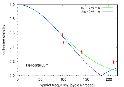
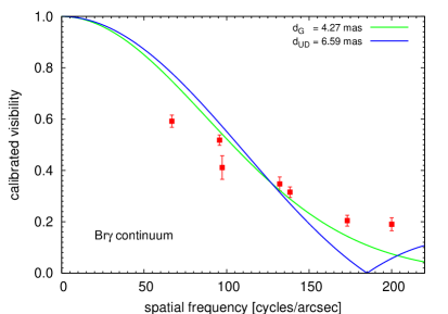
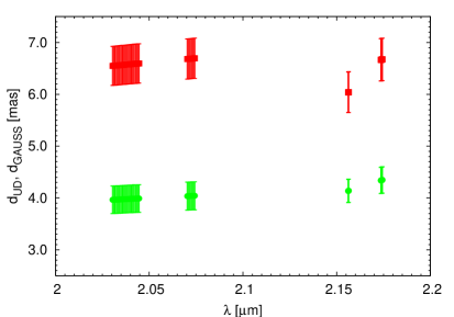
Figure 13: 1-D visiblity fits of the AMBER continuum measurements. The upper two panels show uniform-disk and Gaussian fits for the averaged continuum around the He I and Br$\gamma$ lines, respectively. As both panels illustrate, neither a uniform disk nor a Gaussian is a good representation of the AMBER measurements. The panel on the left summarizes the fitting attempt for all continuum wavelength channels by displaying the fitted diameters of the UD and GAUSS models as a function of wavelength.

For each spectral channel as well as for an averaged continuum, we performed 1-D fits to the visibility data using simple uniform disk (UD) and Gaussian models. In this step of the analysis, possible asymmetries were ignored and all visibility points at a given wavelength were fitted together, regardless of the position angle of the observations. The results of these 1-D fits are illustrated in the two upper panels of Fig. 13 for the averaged continuum data in the wavelength ranges 2.03–2.08$\,\mu$m and 2.155–2.175$\,\mu$m, respectively. As the figure reveals, neither a uniform disk nor a single Gaussian provides a good fit to the continuum data. At least, this is true as long as no contamination by a fully resolved background component is taken into account.

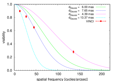
Figure 14: Dependence of the Gaussian FWHM diameter on the fit range. The figure shows the background-corrected visibilities obtained with VLTI/VINCI (see van Boekel et al. 2003) as well as Gaussian fits of (a) all four data points (long-dashed green line), (b) only the point with $q=45\,$ cycles/arcsec (short-dashed blue), (c) only the point corresponding to the longest baseline (dotted purple), and (d) only the point corresponding to the shortest baseline (dashed-dotted light blue). See the labels for the Gaussian FWHM diameters resulting from the different fits. The figure illustrates that the fitted diameter strongly depends on the spatial frequency range which is used to fit the data. The strong diameter variation (in this case, the diameter changes by a factor of $\sim 3$) occurs since a Gaussian is not a good representation of the measured visibility function. See text for further discussion.

The wavelength dependence of the apparent size obtained from the UD and GAUSS model fits for the individual spectral channels is shown in the lower left panel of Fig. 13. This panel illustrates that the equivalent UD and GAUSS $K$-band diameters of $\eta$ Car derived from the AMBER data are $\sim$4 and $\sim$6.5 mas, respectively.

It should be added here that a good fit of the AMBER data using, for instance, a Gaussian can indeed be obtained when a certain amount of contamination due to a fully resolved background component is taken into account (see also Petrov et al. 2006a). To illustrate that, we performed Gaussian fits to the AMBER data, where we introduced such a fully resolved component as a free fitting parameter. We found that the best Gaussian fit is obtained with a FWHM diameter $d_{\rm Gauss}=3.01$ mas and a $\sim 29\%$ background contamination for the He I continuum region and $d_{\rm Gauss}=3.32$ mas and a $\sim 30\%$ background contamination for the Br$\gamma$ continuum region. Thus, from this fit we would derive a background contamination which is only $\sim 50\%$ smaller than in the VINCI data. We think that such a large amount of background contamination is not very likely given the small AMBER fiber aperture (60 mas) of the 8.2 m telescopes. We think that the large amount of background contamination needed to find a reasonable Gauss fit just reflects the fact that a Gaussian is not appropriate to describe the observations. This is confirmed by the fact that for the fit of the radiative transfer model of Hillier et al. (2001), no background component has to be taken into account to reproduce the AMBER measurements.

We would like to note here that the Gaussian FWHM diameters of typically $\sim 4$ mas found from the AMBER measurements are not in contrast to the value $d_{\rm Gauss}\sim 7$ mas found by van Boekel et al. (2003) from VLTI/VINCI observations for the following reason: Since a Gaussian is not a good representation of both the VINCI and the AMBER visibilities, the diameter resulting from a Gaussian fit strongly depends on the fit range. This is illustrated in Fig. 14 for the four VINCI measurements given in Fig. 1 of van Boekel et al. (2003). As the figure shows, from a Gaussian fit of all four data points, $d_{\rm Gauss}=6.0$ mas is obtained. If only the data point with $q=45\,$ cycles/arcsec is fitted (corresponding to a projected baseline length of $\sim 24$ m), we get $d_{\rm Gauss}=7.65$ mas. This is in agreement with the values given in van Boekel et al. (2003) for the elliptical Gaussian fit of the large number of VINCI measurements with a projected baseline of 24 m (see their Fig. 2). On the other hand, if we fit only the VINCI data point corresponding to the longest projected baseline ($q=136\,$ cycles/arcsec), a Gaussian fit provides $d_{\rm Gauss}=4.39$ mas (see Fig. 14), which is very close to the diameter we obtain from the AMBER measurements for $\lambda\sim 2.174\,\mu$m ($d_{\rm Gauss}=4.35$ mas). This is not surprising since the spatial frequency of this VINCI data point agrees with the average spatial frequency of our AMBER observations ($q\sim$50–200 cycles/arcsec). Thus, it can be concluded that good agreement between the Gaussian FWHM diameters derived from the AMBER and VINCI measurements is found if a comparable spatial frequency range is used for the fit.

Appendix C Visibility and differential phase of an emission line object

We assume that the target’s intensity distribution can be described by two components: the continuum spectrum $o_{\rm cont}(x,y;\lambda)$ and the emission line spectrum $o_{\rm line}(x,y;\lambda)$. In the part of the spectrum containing the emission line, both $o_{\rm cont}$ and $o_{\rm line}$ contribute to the total intensity distribution $o_{\rm tot}$. According to the van-Zittert-Zernike theorem, the Fourier transforms $O_{\rm cont}(B/\lambda)$ and $O_{\rm line}(B/\lambda)$ of $o_{\rm cont}(x,y;\lambda)$ and $o_{\rm line}(x,y;\lambda)$ are measured with an optical long baseline interferometer at wavelength $\lambda$ and projected baseline vector $B$. In the following, we assume that all Fourier spectra are normalized to 1 at frequency zero. The complex Fourier spectrum $O_{\rm tot}(B/\lambda)$ of the intensity distribution $o_{\rm tot}$ measured at the emission line $\lambda_{\rm line}$ is given by

$$O_{\rm tot}=\frac{1}{F_{\rm cont}+F_{\rm line}}(F_{\rm cont}\cdot O_{\rm cont}+F_{\rm line}\cdot O_{\rm line}),$$ (3)

where $F_{\rm cont}$ and $F_{\rm line}$ are the fluxes of the continuum component $o_{\rm cont}$ and the line component $o_{\rm line}$, respectively. In the emission line, the total flux measured is $F_{\rm tot}:=F_{\rm cont}+F_{\rm line}$.

¿From the spectrally dispersed interferometric data, we can derive the differential phase, which is the difference of the Fourier phases of the continuum component $o_{\rm cont}$ and the total intensity $o_{\rm tot}$ in the emission line. The differential phase $\Phi^{\prime}(B/\lambda_{\rm line})$ in the emission line at $\lambda_{\rm line}$ is given by

$$O_{\rm cont}\cdot O_{\rm tot}^{*}=V_{\rm cont}\cdot V_{\rm tot}\cdot e^{i\,\Phi^{\prime}},$$ (4)

where $\Phi^{\prime}(B/\lambda_{\rm line}):=\Phi_{\rm cont}(B/\lambda_{\rm line})-\Phi_{\rm tot}(B/\lambda_{\rm line})$. $\Phi_{\rm cont}(B/\lambda_{\rm line})$ is the Fourier phase of the continuum component, and $\Phi_{\rm tot}(B/\lambda_{\rm line})$ denotes the Fourier phase of $o_{\rm tot}$ at the position of the emission line $\lambda_{\rm line}$. The asterisk ^∗ in this equation denotes conjugate complex operation. $V_{\rm cont}(B/\lambda_{\rm line})$ describes the visibility of the continuum component at the position of the emission line $\lambda_{\rm line}$, and $V_{\rm tot}(B/\lambda_{\rm line})$ is the visibility measured at the position of the emission line $\lambda_{\rm line}$. Inserting Eq. (3) into Eq. (4) yields

$$V_{\rm cont}\cdot V_{\rm tot}\cdot e^{i\,\Phi^{\prime}}\\$$

$$=\frac{V_{\rm cont}}{F_{\rm cont}+F_{\rm line}}\cdot(F_{\rm cont}V_{\rm cont}+F_{\rm line}V_{\rm line}e^{i\,\Delta\Phi}),$$ (5)

where $\Delta\Phi(B/\lambda_{\rm line})$ denotes the difference of the Fourier phases of the continuum and line components; i.e., $\Delta\Phi(B/\lambda_{\rm line}):=\Phi_{\rm cont}(B/\lambda_{\rm line})-\Phi_{\rm line}(B/\lambda_{\rm line})$. $\Phi_{\rm cont}(B/\lambda_{\rm line})$ and $\Phi_{\rm line}(B/\lambda_{\rm line})$ are the Fourier phases of the continuum and line components, respectively.

In the vector representation of complex numbers, the three quantities $F_{\rm cont}V_{\rm cont}$, $F_{\rm line}V_{\rm line},$ and $F_{\rm tot}V_{\rm tot}$ form a triangle with one corner placed at the center of the coordinate system. According to the law of cosines, the correlated flux of the line component is given by Eq. (2) (see Sect. 3.4.1):

$$|F_{\rm line}V_{\rm line}|^{2} =|F_{\rm tot}V_{\rm tot}|^{2}+|F_{\rm cont}V_{\rm cont}|^{2}-$$ (6)

$$-2\cdot F_{\rm tot}V_{\rm tot}\cdot F_{\rm cont}V_{\rm cont}\cdot{\rm cos}(\Phi^{\prime}).$$

Since the flux $F_{\rm line}$ can be calculated from the measured fluxes $F_{\rm cont}$ and $F_{\rm tot}$, the visibility $V_{\rm line}$ of the line component can be derived using Eq. (6).

Applying the law of sines to this triangle in the complex plane yields the differential phase $\Delta\Phi(B/\lambda_{\rm line})$, which is the difference between the Fourier phase $\Phi_{\rm cont}(B/\lambda_{\rm line})$ of the continuum component and the Fourier phase $\Phi_{\rm line}(B/\lambda_{\rm line})$ of the line component:

$${\rm sin}(\Delta\Phi)={\rm sin(\Phi^{\prime})}\cdot\frac{|F_{\rm tot}V_{\rm tot}|}{|F_{\rm line}V_{\rm line}|},$$ (7)

where $\Phi^{\prime}(B/\lambda_{\rm line})$ is the differential phase measured at the position of the emission line $\lambda_{\rm line}$.