The VLT-FLAMES survey of massive stars: Surface chemical compositions of B-type stars in the Magellanic Clouds

We present an analysis of high-resolution FLAMES spectra of approximately 50 early B-type stars in three young clusters at different metallicities, NGC 6611 in the Galaxy, N 11 in the Large Magellanic Cloud (LMC) and NGC 346 in the Small Magellanic Cloud (SMC). Using the tlusty non-LTE model atmospheres code, atmospheric parameters and photospheric abundances (C, N, O, Mg and Si) of each star have been determined. These results represent a significant improvement on the number of Magellanic Cloud B-type stars with detailed and homogeneous estimates of their atmospheric parameters and chemical compositions. The relationships between effective temperature and spectral type are discussed for all three metallicity regimes, with the effective temperature for a given spectral type increasing as one moves to a lower metallicity regime. Additionally the difficulties in estimating the microturbulent velocity and the anomalous values obtained, particularly in the lowest metallicity regime, are discussed. Our chemical composition estimates are compared with previous studies, both stellar and interstellar with, in general, encouraging agreement being found. Abundances in the Magellanic Clouds relative to the Galaxy are discussed and we also present our best estimates of the base-line chemical composition of the LMC and SMC as derived from B-type stars. Additionally we discuss the use of nitrogen as a probe of the evolutionary history of stars, investigating the roles of rotational mixing, mass-loss, blue loops and binarity on the observed nitrogen abundances and making comparisons with stellar evolutionary models where possible.

1 Introduction

The differing environments of the Magellanic Clouds, compared with our own Galaxy and with each other, makes them ideal laboratories for the study of both stellar and galactic evolution. Their proximity, combined with their relatively low extinction has contributed to the intensity with which they have been studied in recent years (see, for example, Bouret et al. bou03 (2003); Korn et al. kor02 (2002); Garnett gar99 (1999); Westerlund wes97 (1997)). For stellar evolutionary theories it is necessary that the present-day chemical composition of the host material in which star-birth occurs is well understood. The interstellar material can be directly sampled via, for example, H ii regions (Dufour duf84 (1984); Russell & Dopita rus90 (1990); Peimbert et al. pei00 (2000); Kurt & Dufour kur98 (1998)) but such studies may be complicated by depletion onto dust grains.

Young massive stars allow for an alternative means to determine chemical compositions. However, there is evidence (Gies & Lambert gie92 (1992); Maeder mae87 (1987); Langer et al. lan98 (1998); Heger & Langer heg00 (2000)) that mixing of CN-cycled material into the stellar photosphere can occur giving rise to N enrichment and to smaller C and O underabundances. Nevertheless by selecting targets that do not appear to have had material mixed into their atmospheres, massive stars can provide reliable indicators of the pristine chemical composition of a recent or ongoing star formation region.

An important challenge for theoretical evolutionary predictions is to reliably model the wide range of N/H abundances seen in observations of A-type supergiants (Venn et al. ven99 (1999)) as well as in B-type stars, both supergiant and main-sequence (see, for example, Korn et al. kor02 (2002), Lennon et al. len03 (2003) and Trundle et al. tru04 (2004)). The role of rotational mixing has become increasingly important particularly for main-sequence objects (Maeder & Meynet mae01 (2001), Meynet & Maeder mey02 (2002) and Lamers et al. lam01 (2001)). Futhermore, observational evidence suggests that stellar rotational velocity distributions may depend on metallicity whilst cluster stars may have greater rotational velocities than those in the field (Keller kel04 (2004), Strom et al. str05 (2005)). As the amount of mixing depends on the initial stellar rotational velocity, it is important that these effects are fully understood.

Metallicity plays an important role in all aspects of massive star evolution. For example, at low metallicity the stars are more compact, have lower mass-loss rates (Massey mas03 (2003)) and therefore they may lose less angular momentum and hence may rotate faster (Meynet & Maeder mey02 (2002)). As discussed above, this scenario then leads to enhanced mixing between the stellar interior and surface. Additionally photospheric mixing is more evident at lower metallicity as small absolute changes in the abundances will be easier to observe and hence the Magellanic Clouds provide ideal laboratories within which metallicity effects upon steller evolution can be tested.

Binarity effects have been less studied, both because these effects do not globally affect a given population of stars and also due to the wide range of free parameters that are involved in modelling a binary stystem. However mass-transfer in binary systems may be an important contributor to the abundance variations found between stars within a given population. Additionally, the implications of binarity for other processes such as rotational mixing is not fully understood.

We have undertaken a high resolution spectroscopic survey of young clusters in the Galaxy, LMC and SMC (see Evans et al. eva05a (2005), eva05b (2006)) and observations have been obtained for a total of 750 stars, mainly with O and B spectral types. Mokiem et al. (2006a , 2006b ) have derived atmospheric parameters and rotational velocities of the O-type objects in this survey. In this paper we discuss B-type stars with narrow absorption line spectra in the young Magellanic Cloud clusters, N 11 and NGC 346 along with NGC 6611, a Galactic cluster with a similar age.

We determine atmospheric parameters and abundances (C, N, O, Mg and Si) of approximately 50 early B-type stars in these three clusters with the aim of determining the base-line chemical abundances of each region from a large sample of objects, taking into account any chemical enrichments or depletions which may have occured during the stellar lifetime. Additionally we examine our results in terms of the stellar evolution of these objects, through both internal mixing and binary interaction.

In Sect. 2 we discuss our target selection. In Sect. 3 we discuss our methodology and present the photospheric abundances derived for each star in our sample along with estimates of the uncertainites in these abundances. In Sect. 4 we discuss the elemental abundances and in Sect. 5 we compare our results to previous stellar and interstellar analyses of the three regions. In Sect. 6 we discuss both abundance differences between the three clusters and between stars within the same region, comparing where possible our observations with current evolutionary theory. Finally in Sect. 7 we present our best estimates for the present-day chemical composition of the LMC and SMC and summarize the evolutionary effects observed in the sample.

2 Observations

The target selection, observational details and data reduction procedures for clusters in our Galaxy and in the Magellanic Clouds have been described in Evans et al. (eva05a (2005)) (hereafter Paper I) and Evans et al. (eva05b (2006)) (hereafter Paper II) respectively. In summary, the majority of the observations were obtained using the Fibre Large Array Multi-Element Spectrograph (FLAMES), with R$\approx$20000 at the Very Large Telescope (VLT) as part of a European Southern Observatory (ESO) Large Programme. These were supplemented using the Fiber-fed Extended Range Optical Spectrograph (FEROS), with R$\approx$48000, and the Ultraviolet and Visual Echelle Spectrograph (UVES), with R$\approx$20000. Seven clusters were observed in the Galaxy and the Small (SMC) and Large (LMC) Magellanic Clouds and the high resolution FLAMES spectroscopy covered the wavelength region 3850-4755Å and the H$\alpha$ region 6380-6620Å (with more extensive wavelength coverage for the FEROS and UVES observations). Examples of the quality of the spectra can be found in Papers I and II. In this paper we discuss only stars observed in the youngest cluster in each metallicity regime, viz. NGC 6611 in the Galaxy, N 11 in the LMC and NGC 346 in the SMC.

Table 1: The estimated atmospheric parameters of our sample. Star identifications and spectral types have been taken from Paper I and Paper II. Effective temperatures ($T_{\rm eff})$ are determined from the ionization balance of Si iii to Si iv unless otherwise noted. The surface gravity, g, has units of cm s^-2. Note, in Sect. 3.7.1 we present alternative microturbulence ($\xi$) values based on the derived Si abundance. The uncertainties in these parameters are typically 1 000 K for $T_{\rm eff}$, 0.15–0.20 dex for $\log g$, 3–5 km s^-1 for $\xi_{\rm Si}$ and 5 km s^-1 for $v\sin i$ (see Sect. 3 for details).

Star	Spectral	$T_{\rm eff}$	$\log g$	$\xi_{\rm Si}$	$v\sin i$	$\log L/L_{\sun}$	$M_{\rm evol}/M_{\sun}$	Instrument
	Type	K	dex	km s-1	km s-1
NGC 6611-006	B0 IVp∗	31250	4.00	7	20	4.87	$20^{\rm+3}_{\rm-2}$	FLAMES
NGC 6611-012	B0.5 V	27200	3.90	6	95	4.81	$18^{\rm+2}_{\rm-1}$	FLAMES
NGC 6611-021	B1 V	26250	4.25	0	30	4.38	$13^{\rm+2}_{\rm-1}$	FEROS
NGC 6611-030R	B1.5 V	225001	4.15	5	10	3.63	$8^{\rm+1}_{\rm-1}$	FLAMES
NGC 6611-033	B1 V	25600	4.00	1	25	4.20	$12^{\rm+1}_{\rm-1}$	FLAMES
N 11-001	B2 Ia	187503	2.50	14	50	5.66	$38^{\rm+7}_{\rm-3}$	UVES
N 11-002	B3 Ia	158001	2.10	12	55	5.26	$24^{\rm+3}_{\rm-2}$	UVES
N 11-003	B1 Ia	23200	2.75	13	80	5.42	$30^{\rm+5}_{\rm-3}$	UVES
N 11-008	B0.5 Ia	25450	3.00	15	75	5.39	$30^{\rm+5}_{\rm-3}$	FLAMES
N 11-009R5	B3 Iab	150001	2.15	17	40	4.85	$17^{\rm+2}_{\rm-1}$	FLAMES
N 11-012	B1 Ia	20500	2.55	14	70	5.13	$22^{\rm+2}_{\rm-1}$	FLAMES
N 11-014R5	B2 Iab	191001	2.55	13	50	5.03	$19^{\rm+2}_{\rm-1}$	FLAMES
N 11-015	B0.7 Ib	23600	2.95	11	75	5.23	$24^{\rm+2}_{\rm-1}$	UVES
N 11-016	B1 Ib	21700	2.75	14	60	5.13	$22^{\rm+2}_{\rm-1}$	UVES
N 11-017R5	B2.5 Iab	165001	2.30	17	45	4.82	$17^{\rm+2}_{\rm-1}$	FLAMES
N 11-023	B0.7 Ib	24000	2.90	14	70	5.09	$21^{\rm+2}_{\rm-1}$	UVES
N 11-024	B1 Ib	21600	2.80	12	55	4.96	$18^{\rm+2}_{\rm-1}$	FLAMES
N 11-029	OC9.7 Ib	28750	3.30	11	70	5.21	$25^{\rm+3}_{\rm-2}$	FLAMES
N 11-036	B0.5 Ib	23750	3.10	11	55	4.95	$18^{\rm+2}_{\rm-1}$	FLAMES
N 11-037R	B0 III	28100	3.25	10	100	5.08	$23^{\rm+2}_{\rm-2}$	FLAMES
N 11-042R	B0 III	29000	3.60	6	30	5.05	$22^{\rm+2}_{\rm-2}$	FLAMES
N 11-047R	B0 III	29200	3.65	8	55	5.03	$21^{\rm+2}_{\rm-2}$	FLAMES
N 11-054	B1 Ib	23500	3.05	11	60	4.79	$16^{\rm+2}_{\rm-1}$	FLAMES
N 11-062R	B0.2 V	30400	4.05	5	25	4.95	$21^{\rm+2}_{\rm-2}$	FLAMES
N 11-069	B1 III	24300	3.30	10	80	4.63	$15^{\rm+1}_{\rm-1}$	UVES
N 11-072	B0.2 III	28800	3.75	5	15	4.77	$18^{\rm+2}_{\rm-2}$	FLAMES
N 11-075R	B2 III	218003	3.35	3	25	4.48	$12^{\rm+1}_{\rm-1}$	FLAMES
N 11-083R	B0.5 V	29300	4.15	0	20	4.71	$17^{\rm+2}_{\rm-1}$	FLAMES
N 11-100	B0.5 V	29700	4.15	1	30	4.68	$17^{\rm+2}_{\rm-1}$	UVES
N 11-101	B0.2 V	29800	3.95	8	70	4.68	$17^{\rm+2}_{\rm-2}$	UVES
N 11-106	B0 V	31200	4.00	7	25	4.72	$18^{\rm+2}_{\rm-2}$	FLAMES
N 11-108	O9.5 V	32150	4.10	7	25	4.73	$19^{\rm+2}_{\rm-2}$	FLAMES
N 11-109	B0.5 Ib	25750	3.20	14	55	4.48	$12^{\rm+2}_{\rm-1}$	FLAMES
N 11-110	B1 III	23100	3.25	6	25	4.37	$12^{\rm+1}_{\rm-1}$	FLAMES
N 11-124R	B0.5 V	28500	4.20	0	45	4.47	$14^{\rm+2}_{\rm-1}$	FLAMES
NGC 346-012	B1 Ib	24200	3.20	8	30	4.77	$16^{\rm+1}_{\rm-1}$	FLAMES
NGC 346-021	B1 III	25150	3.50	1	15	4.61	$14^{\rm+1}_{\rm-2}$	FLAMES
NGC 346-029R	B0 V	32150	4.10	0	25	4.82	$19^{\rm+2}_{\rm-1}$	FLAMES
NGC 346-037	B3 III	188001	3.20	5	35	4.21	$10^{\rm+1}_{\rm-1}$	FLAMES
NGC 346-039R	B0.7 V	25800	3.60	0	20	4.51	$13^{\rm+1}_{\rm-1}$	FLAMES
NGC 346-040R	B0.2 V	30600	4.00	0	20	4.67	$17^{\rm+2}_{\rm-2}$	FLAMES
NGC 346-043	B0 V	33000	4.25	4	10	4.71	$18^{\rm+2}_{\rm-2}$	FLAMES
NGC 346-044	B1 II	230002	3.50	0	40	4.33	$10^{\rm+2}_{\rm-1}$	FLAMES
NGC 346-056	B0 V	31000	3.80	1	15	4.55	$16^{\rm+2}_{\rm-1}$	FLAMES
NGC 346-062	B0.2 V	29750	4.00	12	25	4.45	$15^{\rm+1}_{\rm-1}$	FLAMES
NGC 346-075R	B1 V	27700	4.30	0	10	4.31	$12^{\rm+1}_{\rm-1}$	FLAMES
NGC 346-094	B0.7 V	28500	4.00	4	40	4.28	$13^{\rm+1}_{\rm-1}$	FLAMES
NGC 346-103	B0.5 V	29500	4.00	0	10	4.26	$13^{\rm+1}_{\rm-1}$	FLAMES
NGC 346-116	B1 V	28250	4.10	0	15	4.15	$12^{\rm+1}_{\rm-1}$	FLAMES

• Radial velocity variations detected at the 3$\sigma$ level and hence object may be a binary, see Sect. 2.2. ^R5 indicates that the radial velocity variation is less than 5 km s^-1.

• After the discussion in Paper I, we have since revised the spectral type of NGC 6611-006 to B0 IV; its spectrum is intermediate between those of $\upsilon$ Ori and HD 48434 from Walborn & Fitzpatrick (wal90 (1990)), but with slightly stronger He ii $\lambda$4200 than one would expect.

• $T_{\rm eff}$ estimated from ionization balance of Si ii to Si iii.

• $T_{\rm eff}$ estimated by placing upper limits on the EW of the Si ii and Si iv lines, see Sect. 3.2.1.

• $T_{\rm eff}$ estimates determined from the ionization balance of Si ii to Si iii and Si iii to Si iv are in good agreement.

2.1 Selection of narrow lined stars

The spectra of all the stars with a type later than O9 have been examined and we have selected stars for analysis using the criterion that their metal absorption lines were sufficiently narrow so that they could be easily identified and measured. O-type stars were not considered as they lay outside our grid of model atmosphere calculations (see Sect. 3.1) and are more appropriately modelled with unified stellar wind codes, see for example, Mokiem et al. (2006a , 2006b ).

The spectra were examined for evidence of double-lined binarity, and if contamination from a secondary object was apparent, they were excluded. Additionally stars were only selected for analysis if it was possible to reliably determine their effective temperature. As the clusters are young, many of the stars have early B spectral types and effective temperatures could be deduced using the ionization equilibrium of Si iii to Si iv. For cooler objects (with effective temperatures less than 18 000 K) the ionization equilibrium of Si ii to Si iii could be used. However there was a range of effective temperatures within which both the Si ii and Si iv lines were too weak to measure and the helium spectrum could not be used to constrain the temperature. In these cases if the temperature could not be constrained to better than $\pm$1 000 K by putting limits on the strength of both the Si ii and Si iv lines then the star was not included in our analysis. The methods used to determine the temperatures are further discussed in Sect. 3.2. Due to these selection criteria and the low metallicity of the SMC it was only normally possible to analyse stars in NGC 346 with a maximum projected rotational velocity of approximately 50 km s^-1. As the absorption lines are stonger in the LMC and Galactic stars, and also as we have several supergiant objects in the LMC sample, stars with an implied projected rotational velocity of up to 100 km s^-1 could be analysed in NGC 6611 and N 11.

An additional selection criterion was whether the spectra were of sufficient quality to reliably measure the equivalent widths (EW) for absorption lines from several chemical species. The Si iii triplet of lines at 4560Å was observed in two wavelength orders leading to independent estimates for their equivalent widths. Objects have only been included in this analysis if agreement between the EW’s from the two orders was better than 10%. Table 1 lists all the stars that were selected for analysis based on these criteria. Star identifications have been adopted from Paper I and Paper II for the Galactic stars and Magellanic Cloud stars respectively and alternative identifications along with radial velocity estimates can be found therein. It should be noted that this analysis represents only a subset of the B-type objects observed in the survey as some objects lay outside our strict selection criteria.

2.2 Equivalent Width Measurements

Several exposures were taken for each cluster in each wavelength setting and these are summarized in Table 2. Spectra in each wavelength setting were cross-correlated and corrected for any resulting velocity shifts. In several wavelength settings the exposures were taken in two sets of three at different dates and stars were identified as possible single lined spectroscopic binary objects if the mean radial velocity of each set of exposures differed at the 3$\sigma$ level, see Table 1. Of course, especially for small radial velocity variations binarity is not the only explanation; pulsations or uncertainties in the wavelength calibrations may also contribute to variations. Additionally, wind effects can lead to a change in the line profiles and hence spurious radial velocity variations may be detected, especially in the redder wavelength regions. As such we do not include objects as radial velocity variables in Table 1 if changes in the shape of the line profile were also observed. Generally, velocity shifts could be identified to an accuracy of better than 5 km s^-1, except for the brightest targets in N 11 where velocity shifts of less than 2 km s^-1 could be detected. For the targets not observed with FLAMES only a single exposure was available and hence it was not possible to examine these objects for evidence of binarity.

The individual exposures in each wavelength region were then combined using IRAF routines which also removed most cosmic ray events. The combined FLAMES spectra had signal to noise (S/N) ratios per pixel ranging from 60 to in excess of 400 with the majority of the NGC 6611 and NGC 346 stars having S/N ratios greater than 100 and the majority of the N 11 targets having S/N ratios greater than 200. The single spectrum in this sample which was obtained with FEROS had a S/N ratio of 80, while those from UVES had S/N ratios ranging from 60-110.

The combined spectra were normalised within the spectral analysis package dipso (Howarth et al. how94 (1994)) and the line fitting program elf was used to measure the EW of the absorption lines by fitting Gaussian profiles to the line and using a low order polynominal to represent the continuum. As discussed above, we estimated the error in the EW of well observed unblended Si iii features to be better than 10%. For weak or blended features an error of 20% may be more appropriate. EW measurements of the absorption lines in the spectra of each star listed in Table 1 are given in Table 3, Table 4 and Table 5 (only available online at the CDS) for NGC 6611, N 11 and NGC 346 respectively. In these tables we also list the ionic species, the rest wavelength and the derived abundance of each absorption line. Lines with measured equivalent widths and no corresponding abundance estimate were cases where reliable theoretical calculations were not available.

Table 2: Number of exposures taken by the FLAMES spectrograph in each wavelength setting. See Papers I and II for further details.

Setting	Central	Number of exposures
	Wavelength (Å)	NGC 6611	N 11	NGC 346
HR02	3958	2	6	6
HR03	4124	2	6	6
HR04	4297	2	6	6
HR05	4471	4	6	6
HR06	4656	4	6	8
HR14	6515	4	6	9

3 Analysis

3.1 Non-LTE atmosphere calculations

Non-LTE model atmosphere grids generated using tlusty and synspec (Hubeny hub88 (1988); Hubeny & Lanz hub95 (1995); Hubeny et al. hub98 (1998)) were used throughout this analysis to derive atmospheric parameters and chemical abundances. An overview of the methods can be found in Hunter et al. (hun05 (2005)) while a more detailed discussion of the methods and grids can be found in Ryans et al. (rya03 (2003)) and Dufton et al. (duf05 (2005)). The adopted atomic data is listed in Table 6 (only available online at the CDS). In this table we list the species, wavelength, $\log gf$ value and also indicate if the line is considered as part of a blend of lines in the TLUSTY code, see Dufton et al., Allende Prieto et al. all03 (2003) and Lanz & Hubeny lan03 (2003) for details.

Briefly, four model atmosphere grids have been calculated for metallicities correponding to a Galactic metallicity of [Fe/H]=7.5 dex, and metallicities of 7.2, 6.8 and 6.4 dex to represent the LMC, SMC and lower metallicity material respectively (see for example, Gies & Lambert gie92 (1992), Luck & Lambert luc92 (1992), Bouret et al. bou03 (2003) and Lehner leh02 (2002)). For each of these grids non-LTE models have been calculated for effective temperatures ranging from 12 000K to 35 000K, in steps of no more than 2 500K, surface gravities ranging from 4.5 dex down to the Eddington limit, in steps of no more than 0.25 dex and for microturbulences of 0, 5, 10, 20, and 30 km s^-1. Assuming that the light elements (C, N, O, Mg and Si) have a negligible effect on line-blanketing and the structure of the stellar atmosphere, models were then generated with the light element abundance varied by +0.8, +0.4, -0.4 and -0.8 dex about their normal abundance at each point on the tlusty grid. A helium abundance of 11.0 dex has been adopted throughout these grids and the implication of this with respect to our sample of stars is discussed in Sect. 4.1. Theoretical spectra and EW’s were then calculated based on these models. Photospheric abundances for approximately 200 absorption lines at any particular set of atmospheric parameters covered by the grid can then be calculated by interpolation between the models via simple IDL routines. The reliability of the interpolation technique has been tested by Ryans et al. (rya03 (2003)) and they report that no significant errors arise from it.

3.2 Stellar Atmospheric Parameters

A static stellar atmosphere is normally characterised by four parameters, viz. the effective temperature, surface gravity, microturbulence and metallicity. These parameters are interdependent and hence it is necessary to use an iterative method to estimate them. The metallicity (iron content) was assumed to be constant for each cluster, i.e. Galactic metallicity ([Fe/H] = 7.5 dex) for NGC 6611, and reduced by 0.3 dex and 0.7 dex for N 11 and NGC 346 respectively. Hunter et al. (hun05 (2005)) and Dufton et al. (duf05 (2005)) have found that these assumptions do not normally cause a significant uncertainty in the estimation of the atmospheric parameters or derived abundances and this is further discussed in Sect. 3.7.1. By careful selection of the initial parameters (based on the spectral types from Paper I or estimates given in Dufton et al. duf06 (2006)), relatively few iterations were necessary to derive the effective temperature, surface gravity and microturbulence. The atmospheric parameters that were adopted for each star are given in Table 1.

3.2.1 Effective Temperature

Given the age of the clusters, the majority of the targets have early B spectral types and therefore the ionization equilibrium of Si iii to Si iv could be used to estimate the effective temperature ($T_{\rm eff}$), see for example, Kilian et al. (kil91 (1991)). Temperatures were rounded to the nearest 50 K which resulted in an imbalance of up to 0.04 dex between the abundances of two Si ionization states. For the hottest objects, the He ii spectrum provided an additional criterion. The values derived using the two methods were in good agreement, with differences normally being less than 1 000 K. While this agreement is encouraging, in most cases the estimates derived from the He ii lines were systematically higher than those from the silicon lines. For example, in Fig. 1 we plot the He ii line for a typical case (NGC 346-040) where the temperature implied by the He ii line spectra is several hundred Kelvin higher than that estimated from the silicon lines.

Additionally atmospheric parameters of several of our Magellanic Cloud objects have been independently estimated by Mokiem et al. (2006a , 2006b ) using the non-LTE code fastwind (Puls et al. pul05 (2005)). In their analysis they adopt an alternative method of fitting the hydrogen and helium spectra to estimate effective temperatures and surface gravities and in all cases higher values were derived compared to the results given here. As values estimated for these atmospheric parameters are directly correlated, the higher gravity probably simply arises from a higher effective temperature estimate. We have derived effective temperatures using a similar method (i.e. fitting the He ii line at 4542Å) and our results are listed in Table 7 and compared to those of Mokiem et al. with the two sets of estimates now being in better agreement. We therefore attribute the differences between our adopted atmospheric parameters and those of Mokiem et al. to the choice of methodology. However, Mokiem et al. (mok05 (2005)) have noted that their genetic algorithm method of determining the atmospheric parameters systematically derives higher gravities than those estimated ‘by-eye’ and hence, given the correlation between the atmospheric parameters, this may contribute to the difference in the temperature estimates.

Dufton et al. (duf06 (2006)) have derived an effective temperature of 34 000 K for NGC 6611-006 using the fastwind code to model the He ii spectrum. Using the He ii 4542Å line we obtain an effective temperature of 33 000 K, 1 750 K higher than that given in Table 1 and in reasonable agreement with Dufton et al. As the He ii line can only be used to estimate the temperature of a small proportion of our sample, we have elected to adopt the estimates from the Si iii to Si iv ionization equilibrium wherever possible in order to maintain consistency throughout this analysis.

Table 7: Comparison of the atmospheric parameters listed in Table 1 with those derived by Mokiem et al. (2006a , 2006b ). For these stars, we also estimate the effective temperature from the He ii line at 4542Å and re-iterate the surface gravity where necessary. Errors in our estimate of the effective temperature from the He ii spectra are typically about 1 500 K.

Star	From Table 1		Mokiem et al.		He ii 4542Å line
	$T_{\rm eff}$	$\log g$	$T_{\rm eff}$	$\log g$	$T_{\rm eff}$	$\log g$
N 11-008	25450	3.00	26000	3.00	25500	3.00
N 11-029	28750	3.30	29400	3.25	29000	3.30
N 11-036	23750	3.10	26300	3.30	25500	3.25
N 11-042	29000	3.60	30200	3.70	29500	3.60
N 11-072	28800	3.75	30800	3.80	30500	3.75
NGC 346-012	24200	3.20	26300	3.35	25500	3.25

Figure 1: Observed spectra for the He ii 4542Å line in NGC 346-040. Theoretical spectra for temperatures of 30 500 K, 31 000 K and 31 500 K (upper, middle and lower smooth curves respectively) are also plotted. The effective temperature deduced from the Si iii to Si iv ionization equilibrium is 30 600 K.

For our coolest objects, the ionization equilibrium of Si ii to Si iii could be used to determine the effective temperature. For our Magellanic Cloud targets, the resulting silicon abundances (see Table 9) appeared to be consistent with those estimated for our hotter targets. For the one Galactic object (NGC 6611-033), the abundance appeared to be underestimated although this may be due to uncertainties in the microturbulence as discussed in Sect. 3.2.3 and Sect. 3.7.1

Three stars in our sample, N 11-001, N 11-014 and N 11-075, reveal measureable Si lines from all three ionization stages and this allows us to compare the effective temperature derived from the ionization balance of Si ii/Si iii to that derived from Si iii/Si iv. In the case of N 11-014 inspection of the models reveals that the results for Si iv become unstable at its estimated surface gravity, which is close to the Eddington limit. These instablilites do not appear to be as serious for Si ii or Si iii spectra and hence we have elected to use these ions to estimate the effective temperature of this star. For N 11-001 and N 11-075, we find that the estimated effective temperatures from the two ionization equilibria agree to within 200 K, highlighted by the almost identical abundance derived for Si from the three ionization stages (see Table 9). This agreement is encouraging as it again indicates that additional errors should not be present when comparing stars where the temperatures have been derived using different ionization stages of silicon.

In some cases (especially at low metallicity) neither the Si ii or the Si iv lines could be observed. By placing upper limits on their equivalent widths, lower and upper limits to the effective temperature could be estimated (see for example, Trundle et al. tru04 (2004)). As discussed in Sect. 2.1, these differed by less than 2 000 K and their mean was adopted. Carbon was the only other element for which two ionziation stages were available, but given the very simple C iii model atom that was used in the tlusty grid, the C ii/C iii ionization equilibrium is probably not a reliable temperature estimator. We discuss the modelling of the carbon spectra further in Sect. 4.2.

On the basis of the quality of the observed spectra and the agreement between the different criteria adopted, we believe that the typical uncertainty in our effective temperature estimates should be of the order of $\pm$1 000K.

3.2.2 Logarithmic Surface Gravity

The logarithmic surface gravity ($\log g$) of each star was estimated by fitting the observed hydrogen Balmer lines with theoretical profiles. Automated procedures have been developed to fit model spectra in our tlusty model atmosphere grid to the observed spectra, with contour maps displaying the region of best fit. If an effective temperature estimate was available, (e.g. from the methods described above), it was a simple matter to estimate the gravity. This could then be used to re-iterate for our effective temperature estimate. For several of the supergiants in N 11 (N 11-001, N 11-003, N 11-008, N 11-016) our gravity estimate lay near to the edge of our grid and our atmospheric parameters and abundance estimates should be treated with some caution.

In order to quantify the uncertainty in our gravity estimate arising from both our normalisation and fitting procedures, we have derived the surface gravity from both the H_δ and H_γ lines. Normalisation of the hydrogen lines for the stars in NGC 6611 was complicated by the relatively strong metal absorption lines in the wings of the H lines but this was less of a problem for the lower metallicity stars in N 11 and NGC 346. Nevertheless, the surface gravity estimates from the two hydrogen lines were in agreement to typically better than 0.1 dex for high gravity stars and 0.05 dex for the supergiants. Fig. 2 shows the agreement of the gravity estimate between the H$\delta$ and the H$\gamma$ line for a main-sequence and a giant star. The uncertainty in the effective temperature estimate would typically contribute an additional uncertainty of 0.1 dex.

Figure 2: (a) and (b) show the quality of the model fit onto the observed H$\delta$ and H$\gamma$ lines of NGC 346-043 (a slowly rotating B0 V with a $v\sin i$ of 10 km s^-1). Similarly, (c) and (d) show the fitting of the same hydrogen lines for N 11-037 (a fast rotating B0 III star with a $v\sin i$ of 100 km s^-1). The smooth curves represent the models. Note, the model spectra shown only includes data for the H-lines and excludes those due to metals.

3.2.3 Microturbulence

The microturbulence is normally derived by removing the dependence of the abundance estimates for lines of a specific ion on line strength. For B-type stars, the O ii ion is often considered (for example, Simón-Díaz et al. sim06 (2006), Hunter et al. hun05 (2005), Gies & Lambert gie92 (1992), and Daflon et al. daf04 (2004)) as its rich spectrum should improve its reliablity. However its use is complicated by the lines arising from different multiplets, making any estimate susceptible to errors in the adopted atomic data or in the magnitude of non-LTE effects. In order to remove these uncertainties, a single O ii multiplet can be used, but then one is reduced to using relatively few lines. While this was possible for the sharpest lined NGC 6611 stars, it was not always feasible in the lower metallicity environments of N 11 and NGC 346 as the weakest line in any multiplet often could not be identified. In order to maintain consistency throughout the analysis we have instead initially estimated the microturbulence ($\xi_{\rm Si}$) from the Si iii triplet of lines at 4552–4574Å as these lines could be seen in all our spectra. As these lines are from the same multiplet, errors arising from the oscillator strengths and departure co-efficients will be negligible and this method has been used previously by, for example, Dufton et al. (duf05 (2005)) and Vrancken et al. (vra97 (1997), vra00 (2000)).

As the derived microturbulence depends on the adopted equivalent widths, we have investigated the effect of changing these by their estimated errors (10% in the case of strong lines, and by 5 mÅ for lines with EW’s of less than 50 mÅ). Typically such errors lead to an uncertainty in the microturbulence estimate of approximately 3 km s^-1, although for stars with higher microturbulences (where the derived abundances are less sensitive to microturbulence) an error of 5 km s^-1 is probably more realistic.

Previous studies (such as Daflon et al. daf04 (2004)) have shown that the microturbulence generally increases as surface gravity decreases and in Fig. 3 we plot our estimates against surface gravity for all the stars listed in Table 1. The largest sample of stars comes from the LMC and these stars also have the widest range of gravities. From Fig. 3 it can be seen that the LMC stars show a strong trend of increasing microturbulence as surface gravity decreases for surface gravities less than 3.3 dex. However, at gravities greater than 3.3 dex there is a much greater scatter, and little evidence of any correlation with gravity; hence Fig. 3 could be interpreted as a bi-modal distribution. Only five near main-sequence stars were analysed in NGC 6611 and hence it is not possible to identify any trend. The 14 targets in NGC 346 cover a relatively wide range of gravities (from 3.2 dex to 4.3 dex), but no trend is apparent which is in agreement with the higher gravity LMC stars.

Examination of the location of the SMC stars in Fig. 3 reveals two important results. Firstly, seven SMC stars were assigned a microturbulence of 0 km s^-1. Furthermore, in some cases adopting this value was not sufficent to remove the dependence of the abundance upon line strength, in the sense that the weakest line of the multiplet still gave the highest abundance. If we adjusted the EW’s of the silicon lines by their assumed errors, a zero microturbulence could be obtained. However given that this discrepancy occured in four out of the seven SMC stars assigned a zero microturbulence, this is not a convincing explanation. Rather, there may be other physical processes occuring which affect the curve-of-growth of a given multiplet but which may be dominated (or at least masked) by the microturbulence parameter at higher metallicity.

Secondly, examination of Fig. 3 reveals stars in NGC 346 with surface gravities of 4.0 dex and similar effective temperatures of approximately 30 000 K, two of which have microturbulences of 0 km s^-1 (NGC 346-103 and NGC 346-040) whilst one of the others has a microturbulence of 12 km s^-1 (NGC 346-062). In order to determine if this is a real effect, the EW of the Si iii lines have again been adjusted by their assumed errors in order to derive the lowest possible microturbulence for the case of NGC 346-062 (5 km s^-1) and higher microturbulences for the other two cases (5 km s^-1 and 1 km s^-1 for NGC 346-103 and NGC 346-040 respectively). However, if we adopt these microturbulences the spread in silicon abundance estimates between the three stars increases. Assuming that all three stars should have the same silicon abundance, would indicate that our original microturbulence estimates given in Table 1 are more reliable at least for abundance determinations. Such differences in the microturbulence estimate for stars with similar effective temperatures and gravities and situated in the same cluster (and hence, with similar metallicity and age) is worrying. This again could imply that there are other physical processes within the stellar photosphere that are affecting the shape of the curve-of-growth but are not fully included in our models. Such differences in microturbulence estimates are not found to such an extent in the higher metallicity environments of our N 11 and NGC 6611 sample.

The choice of microturbulence is more critical when estimating abundances from stronger lines and hence will be most important for the Galactic cluster, NGC 6611. In the lowest metallicity region, NGC 346, the microturbulence may be more uncertain for the reasons discussed above, but the derived abundances will be less dependent upon our estimate.

Figure 3: Microturbulence against surface gravity for all stars listed in Table 1. The points plotted as diamonds inside diamonds represent two stars lying at the same position on the graph.

3.2.4 Microturbulence estimated from other species

Although we have adopted the microturbulence from the silicon lines, we have investigated how using alternative species would change our adopted values. As discussed above, two methods are available to us, viz. we can use all the lines of a species or only lines from a single multiplet. Given the wealth of O ii lines observed in our spectra it would normally be expected that any derived microturbulence parameter could be more reliably deduced than when using a single multiplet. However as discussed above this is complicated by the uncertainties arising from the adopted atomic data and non-LTE departure coefficients (see Simón-Díaz et al. sim06 (2006) for a detailed discussion). Normally including all the oxygen lines (apart from those that are close blends) gives significantly higher microturbulences. Indeed, Vrancken et al. (vra97 (1997), vra00 (2000)) report differences of up to 9 km s^-1 between the microturbulence derived from the O ii lines and that derived from the Si iii lines. As a typical example, the oxygen abundances from the O ii spectrum in N 11-075 have been plotted as a function of line strength in Fig. 4, adopting the microturbulence from Table 1. The linear least squares fit implies that the microturbulence should be increased in order to remove the apparent dependence of abundance upon line strength. However, given that the uncertainty due to the scatter in this figure is greater than the gradient of the best-fitting line, the credibility of any derived microturbulence must be questionable. Nevertheless, we find that a microturbulence of 6 km s^-1 would remove the dependence but would not significantly reduce the scatter. Adopting this larger microturbulence reduces the oxygen and silicon abundances by 0.1 dex and 0.3 dex respectively but has little effect on the other abundances.

Figure 4: O ii abundance against line-strength for each O ii line observed in the spectra of N 11-075. The oxygen abundance has been derived using the parameters given in Table 1. Blends of lines have not been included in this figure.

We have also investigated the effect of using a single multiplet of a species to derive the microturbulence for N 11-075. Ideally this would be the best approach for each individual species but in several cases (e.g. Mg ii, C ii) there are insufficient lines from any single multiplet. Nevertheless, for the sake of this comparison we have estimated the microturbulence from both an oxygen and a nitrogen multiplet for N 11-075. The multiplet of O ii lines at 4072Å, 4076Å and 4079Å is the most suitable oxygen multiplet as it has the largest range of line strengths of those observed. Using this, we find a microturbulence of 2 km s^-1, which is 4 km s^-1 smaller than the values found from using all the O ii lines and in reasonable agreement with the value of 3 km s^-1 deduced from the Si iii multiplet. The only multiplet of N lines available to us are the lines at 4601Å, 4614Å and 4630Å and this multiplet has a relatively small spread of EW’s. This multiplet gives an estimated microturbulence of 2 km s^-1, which again is in good agreement with the microturbulence derived using the O ii and Si iii multiplets. Given this agreement it seems reasonable to adopt the microturbulence estimate from the Si iii multiplet which is seen in all of our stellar spectra.

3.3 Luminosity

Luminosities for each star are given in Table 1. For our NGC 6611 targets these have been adopted from Dufton et al. (duf06 (2006)). However, if we adopt the same methodology as Dufton et al. to calculate the reddening towards the Magellanic Cloud stars, (i.e. using observed and intrinsic colours) this leads to unphysical negative values in some cases. Given the low extinction towards the Magellanic Clouds it appeared to be more appropriate to adopt a single value for N 11 and NGC 346.

For NGC 346 we adopt an $E(B-V)$ value of 0.09 (Massey et al. mas95 (1995)) and $A_{\rm V}$ = 2.72$E(B-V)$ (Bouchet et al. bou85 (1985)) with a distance modulus of 18.91 (Hilditch et al. hil05 (2005)) and the bolometric corrections from Vacca et al. (vac96 (1996)) and Bolona (bol94 (1994)). Note that adopting a standard Galactic law of $A_{\rm V}$ = 3.1$E(B-V)$ changes the estimated luminosities by less than 0.03 dex.

N 11 is complicated by containing at least two distinct regions of star formation, LH 9 and LH 10, and Parker et al. (par92 (1992)) give $E(B-V)$ values of 0.05 and 0.17 respectively. Ideally, one would like to associate each star in our sample with either LH 9 or LH 10, but this is further complicated as a significant fraction of the sample may be field stars. As such we have adopted the $E(B-V)$ of 0.13 of Massey et al. (mas95 (1995)) for our LMC targets. The standard law of $A_{\rm V}$ = 3.1$E(B-V)$ together with a distance modulus of 18.56 (Gieren et al. gie05 (2005)) was used in estimating the luminosities.

3.4 Masses

Evolutionary masses are given in Table 1 and have been deduced by interpolating between the evolutionary tracks of Meynet et al. (mey94 (1994)) along with those of Schaller et al. (sch92 (1992)), Schaerer et al. (sch93 (1993)) and Charbonnel et al. (cha93 (1993)) for NGC 6611, N 11 and NGC 346 respectively. The uncertainties are calculated assuming an error of 0.1 dex in $\log L/L_{\sun}$ with the estimated error of 1 000 K in $T_{\rm eff}$ generally having a negligible effect. Non-rotating tracks have been used although as shown by Maeder & Meynet (mae01 (2001)) inclusion of rotation does not significantly affect the derived masses. Additionally it was possible to calculate spectroscopic masses based on the atmospheric parameters and luminosities. However, taking uncertainties of 0.2 dex in $\log g$, 1 000 K in $T_{\rm eff}$ and 0.1 dex in $\log L/L_{\sun}$ we calculate an uncertainty in the spectroscopic mass of approximately 66%, with the uncertainty in the estimated surface gravity dominating this error. Spectroscopic mass estimates are therefore not particularly useful, but within their errors they are consistent with evolutionary masses in the majority of cases.

3.5 FASTWIND analysis of N 11-001 and N 11-002

Mass-loss effects in supergiants may be significant, especially for the most massive stars and hence the plane-parallel static atmosphere that TLUSTY assumes may not be valid. Therefore we have additionally analysed two of the massive supergiants in our sample, N 11-001 and N 11-002, using the unified model atmosphere code FASTWIND and the resulting atmospheric parameters are listed in Table 8.

The atmospheric parameters deduced using the two codes are in reasonable agreement. For N 11-001, the effective temperature disagrees by 1250 K, the gravity by 0.3 dex and the microturbulence by 2 km s^-1 whilst for N 11-002, both codes yield identical estimates. The mass-loss determined from the FASTWIND analyses are 4.5$\times$10^-7 and 2.5$\times$10^-7 M_☉yr^-1 for N 11-001 and N 11-002 respectively. The agreement between TLUSTY and FASTWIND is expected as Dufton et al. (duf05 (2005)) used both codes to derive parameters and abundances for SMC supergiants and found good agreement between the two sets of estimates. As such we can be confident that no additional uncertainties arise from using TLUSTY to analyze the more evolved objects in this sample and hence TLUSTY parameters have been adopted throughout for consistency.

Table 8: FASTWIND parameters of N 11-001 and N 11-002.

	N 11-001	N 11-002
$T_{\rm eff}$(K)	17500	15800
$\log g$ (dex)	2.20	2.10
$\xi_{\rm Si}$ (km s -1)	12	12

3.6 Projected Rotational Velocity

The stellar projected rotational velocity ($v\sin i$) has been estimated using the Si iii triplet as these lines are intrinsically narrow and were observed throughout our sample. For each star, theoretical spectra with atmospheric parameters similar to those listed in Table 1 were selected and their EW’s scaled to those observed. These theoretical lines were then convolved with the appropriate instrumental broadening profiles. IDL procedures have been developed which rotationally broaden this theorectial line profile over a specified range of $v\sin i$ values and these broadened profiles were compared to the observed lines. A chi-squared minimisation test was then performed and the $v\sin i$ value which gave the best fit to the observed absorption line profile was returned. This procedure was carried out for each of the Si iii lines in the 4560Å multiplet and the agreement between the three lines was usually better than 5 km s^-1. From Table 1, it can be seen that the stars in N 11 have a larger distribution of $v\sin i$ values than in the other clusters but this is simply a consequence of N 11 containing a proportionally larger number of high luminosity stars. It should be noted that we have not considered other possible broadening mechanisms such as macroturbulence (see for example Ryans et al. rya02 (2002)) due to the difficulty of distinguishing such broadening from the rotational broadening through profile fitting. As such the estimates given in Table 1 should be treated as upper limits to the actual projected rotational velocity especially for the higher luminosity targets. The $v\sin i$ values quoted in Table 1 have been rounded to the nearest 5 km s^-1 and an uncertainty of 5 km s^-1 in these values can be considered as appropriate.

3.7 Non-LTE photospheric abundances

The stellar photospheric abundances of carbon, nitrogen, oxygen, magnesium and silicon have been estimated using the non-LTE tlusty model atmosphere grid and the atmospheric parameters listed in Table 1. The abundance derived from each absorption line in the spectra of each star are given in Tables 3-5 (online only; see Sect. 2.2) with the average abundance estimates for each star summarized in Table 9.

3.7.1 Errors in photospheric abundances

The uncertainties given in Table 9 include both the random uncertainties arising from, for example, observational errors and errors in individual oscillator strengths, together with the systematic uncertainties arising from the adopted atmospheric parameters. The random uncertainty was taken to be the standard error in the mean, which is the standard deviation of the abundances derived from each line of a given species divided by the square root of the number of lines observed for that species. In cases where only one line of a particular species was observed (e.g. Mg ii), the random uncertainty was taken to be the standard deviation of the abundances derived for our best observed species, O ii. The random uncertainty will include both measurement errors and random errors in the atomic data. The systematic uncertainties were estimated by changing each of the atmospheric parameters in turn by their associated uncertainty (discussed in the previous sections) and the derived abundances were then compared to the values listed in Table 9 to give an estimate of the error. The random and systematic uncertainties were then summed in quadrature to give the uncertainties listed in Table 9. However, we note that we have not accounted for the correlation between effective temperature and surface gravity in the calculation of the systematic errors and as

Table 9: Absolute abundance estimates, together with their estimated uncertainties. The quantities in parenthesis indicate the number of lines observed of that species. Abundances are presented on the scale 12+log[X/H].

Star	C II		N II		O II		Mg II		Si II		Si III		Si IV
NGC6611-006	7.85 $\pm$ 0.24	(3)	7.59 $\pm$ 0.13	(3)	8.52 $\pm$ 0.17	(28)	7.38 $\pm$ 0.22	(1)			7.46 $\pm$ 0.26	(3)	7.47 $\pm$ 0.32	(2)
NGC6611-012	7.89 $\pm$ 0.23	(1)	7.48 $\pm$ 0.22	(1)	8.50 $\pm$ 0.12	(23)	7.24 $\pm$ 0.21	(1)			7.33 $\pm$ 0.25	(3)	7.30 $\pm$ 0.48	(1)
NGC6611-021	7.82 $\pm$ 0.19	(2)	7.51 $\pm$ 0.11	(3)	8.60 $\pm$ 0.19	(24)	7.24 $\pm$ 0.22	(1)			7.40 $\pm$ 0.31	(3)	7.41 $\pm$ 0.52	(1)
NGC6611-030	7.94 $\pm$ 0.17	(2)	7.58 $\pm$ 0.19	(5)	8.44 $\pm$ 0.31	(29)	7.15 $\pm$ 0.22	(1)	7.15 $\pm$ 0.22	(2)	7.17 $\pm$ 0.31	(3)
NGC6611-033	8.09 $\pm$ 0.19	(2)	7.82 $\pm$ 0.15	(3)	8.69 $\pm$ 0.20	(29)	7.49 $\pm$ 0.21	(1)			7.75 $\pm$ 0.33	(3)	7.75 $\pm$ 0.48	(1)
N11-001	7.29 $\pm$ 0.16	(2)	8.20 $\pm$ 0.23	(5)	8.23 $\pm$ 0.30	(14)	7.12 $\pm$ 0.26	(1)	7.22 $\pm$ 0.27	(2)	7.20 $\pm$ 0.39	(3)	7.23 $\pm$ 0.72	(1)
N11-002	7.66 $\pm$ 0.20	(2)	8.14 $\pm$ 0.31	(6)	8.42 $\pm$ 0.44	(15)	7.18 $\pm$ 0.33	(1)	7.47 $\pm$ 0.33	(2)	7.44 $\pm$ 0.47	(3)
N11-003	7.34 $\pm$ 0.23	(1)	7.09 $\pm$ 0.26	(1)	8.34 $\pm$ 0.11	(17)	7.07 $\pm$ 0.24	(1)			7.17 $\pm$ 0.22	(3)	7.19 $\pm$ 0.60	(1)
N11-008	7.45 $\pm$ 0.09	(3)	7.86 $\pm$ 0.20	(3)	8.27 $\pm$ 0.16	(15)	7.12 $\pm$ 0.23	(1)			7.22 $\pm$ 0.26	(3)	7.22 $\pm$ 0.57	(1)
N11-009	7.55 $\pm$ 0.23	(2)	7.74 $\pm$ 0.30	(5)	8.38 $\pm$ 0.40	(19)	6.95 $\pm$ 0.25	(1)	7.18 $\pm$ 0.24	(2)	7.17 $\pm$ 0.41	(3)
N11-012	7.24 $\pm$ 0.26	(1)	7.69 $\pm$ 0.08	(4)	8.39 $\pm$ 0.17	(19)	7.02 $\pm$ 0.31	(1)			7.10 $\pm$ 0.28	(3)	7.10 $\pm$ 0.67	(1)
N11-014	7.59 $\pm$ 0.17	(2)	7.86 $\pm$ 0.17	(5)	8.26 $\pm$ 0.28	(26)	7.15 $\pm$ 0.25	(1)	7.13 $\pm$ 0.28	(2)	7.12 $\pm$ 0.39	(3)	6.73 $\pm$ 0.70	(1)
N11-015	7.45 $\pm$ 0.30	(1)	7.14 $\pm$ 0.30	(1)	8.36 $\pm$ 0.11	(20)	7.01 $\pm$ 0.30	(1)			7.21 $\pm$ 0.25	(3)	7.23 $\pm$ 0.62	(1)
N11-016	7.52 $\pm$ 0.23	(1)	7.86 $\pm$ 0.09	(4)	8.27 $\pm$ 0.17	(17)	7.25 $\pm$ 0.26	(1)			7.05 $\pm$ 0.26	(3)	7.07 $\pm$ 0.55	(1)
N11-017	7.49 $\pm$ 0.26	(1)	7.86 $\pm$ 0.28	(6)	8.32 $\pm$ 0.37	(23)	6.98 $\pm$ 0.23	(1)	7.12 $\pm$ 0.22	(2)	7.15 $\pm$ 0.39	(3)
N11-023	7.45 $\pm$ 0.21	(1)	7.16 $\pm$ 0.24	(1)	8.39 $\pm$ 0.16	(18)	7.00 $\pm$ 0.22	(1)			7.13 $\pm$ 0.24	(3)	7.12 $\pm$ 0.58	(1)
N11-024	7.48 $\pm$ 0.17	(2)	7.85 $\pm$ 0.10	(4)	8.32 $\pm$ 0.20	(22)	7.14 $\pm$ 0.23	(1)			7.15 $\pm$ 0.31	(3)	7.15 $\pm$ 0.58	(1)
N11-029	7.58 $\pm$ 0.40	(1)	7.11 $\pm$ 0.39	(1)	8.31 $\pm$ 0.32	(13)	6.95 $\pm$ 0.33	(1)			7.25 $\pm$ 0.40	(3)	7.26 $\pm$ 0.55	(1)
N11-036	7.32 $\pm$ 0.13	(2)	7.76 $\pm$ 0.12	(4)	8.33 $\pm$ 0.09	(26)	7.03 $\pm$ 0.20	(1)			7.17 $\pm$ 0.24	(3)	7.16 $\pm$ 0.59	(1)
N11-037	7.57 $\pm$ 0.20	(1)	$<$7.18 $\pm$ 0.24	(1)	8.19 $\pm$ 0.20	( 7)	7.02 $\pm$ 0.13	(1)			7.23 $\pm$ 0.31	(3)	7.23 $\pm$ 0.52	(1)
N11-042	7.56 $\pm$ 0.22	(2)	6.92 $\pm$ 0.26	(1)	8.31 $\pm$ 0.18	(21)	7.00 $\pm$ 0.23	(1)			7.14 $\pm$ 0.23	(3)	7.16 $\pm$ 0.52	(1)
N11-047	7.67 $\pm$ 0.26	(1)	$<$6.88 $\pm$ 0.25	(1)	8.24 $\pm$ 0.16	(17)	7.00 $\pm$ 0.24	(1)			7.20 $\pm$ 0.22	(3)	7.19 $\pm$ 0.49	(1)
N11-054	7.51 $\pm$ 0.15	(2)	6.86 $\pm$ 0.13	(2)	8.42 $\pm$ 0.12	(26)	6.97 $\pm$ 0.20	(1)			7.10 $\pm$ 0.23	(3)	7.09 $\pm$ 0.58	(1)
N11-062	7.43 $\pm$ 0.22	(1)	7.16 $\pm$ 0.17	(2)	8.25 $\pm$ 0.14	(26)	6.99 $\pm$ 0.20	(1)			7.16 $\pm$ 0.22	(3)	7.18 $\pm$ 0.47	(1)
N11-069	7.63 $\pm$ 0.25	(1)	6.95 $\pm$ 0.24	(1)	8.47 $\pm$ 0.15	(26)	7.07 $\pm$ 0.24	(1)			7.25 $\pm$ 0.26	(3)	7.23 $\pm$ 0.59	(1)
N11-072	7.46 $\pm$ 0.14	(3)	7.38 $\pm$ 0.08	(3)	8.36 $\pm$ 0.15	(25)	7.12 $\pm$ 0.20	(1)			7.21 $\pm$ 0.24	(3)	7.21 $\pm$ 0.40	(3)
N11-075	7.55 $\pm$ 0.13	(1)	8.11 $\pm$ 0.26	(5)	8.24 $\pm$ 0.30	(25)	7.24 $\pm$ 0.20	(1)	7.32 $\pm$ 0.23	(2)	7.36 $\pm$ 0.38	(3)	7.33 $\pm$ 0.59	(1)
N11-083	7.53 $\pm$ 0.17	(2)	6.86 $\pm$ 0.20	(1)	8.33 $\pm$ 0.10	(27)	7.00 $\pm$ 0.19	(1)			7.06 $\pm$ 0.22	(3)	7.06 $\pm$ 0.45	(1)
N11-100	7.45 $\pm$ 0.25	(1)	7.68 $\pm$ 0.19	(2)	8.38 $\pm$ 0.11	(26)	7.15 $\pm$ 0.25	(1)			7.44 $\pm$ 0.26	(3)	7.45 $\pm$ 0.47	(1)
N11-101	7.74 $\pm$ 0.22	(1)	$<$7.09 $\pm$ 0.22	(1)	8.32 $\pm$ 0.12	21)	7.21 $\pm$ 0.20	(1)			7.16 $\pm$ 0.17	(3)	7.17 $\pm$ 0.46	(1)
N11-106	7.50 $\pm$ 0.28	(1)	7.12 $\pm$ 0.28	(1)	8.31 $\pm$ 0.17	(22)	7.17 $\pm$ 0.24	(1)			7.10 $\pm$ 0.23	(3)	7.10 $\pm$ 0.31	(2)
N11-108	7.66 $\pm$ 0.30	(1)	7.20 $\pm$ 0.32	(1)	8.23 $\pm$ 0.20	(17)	7.12 $\pm$ 0.23	(1)			7.08 $\pm$ 0.26	(3)	7.08 $\pm$ 0.40	(1)
N11-109	7.39 $\pm$ 0.16	(2)	7.22 $\pm$ 0.23	(1)	8.25 $\pm$ 0.12	(17)	6.83 $\pm$ 0.20	(1)			7.01 $\pm$ 0.22	(3)	7.02 $\pm$ 0.51	(1)
N11-110	7.50 $\pm$ 0.20	(1)	7.41 $\pm$ 0.08	(3)	8.54 $\pm$ 0.26	(26)	7.08 $\pm$ 0.20	(1)			7.35 $\pm$ 0.36	(3)	7.36 $\pm$ 0.58	(1)
N11-124	7.56 $\pm$ 0.16	(1)	7.25 $\pm$ 0.17	(1)	8.12 $\pm$ 0.09	(19)	6.97 $\pm$ 0.15	(1)			6.94 $\pm$ 0.21	(3)	6.97 $\pm$ 0.43	(1)

Table 9: –continued.

Star	C II		N II		O II		Mg II		Si II		Si III		Si IV
NGC346-012	7.10 $\pm$ 0.09	(4)	6.93 $\pm$ 0.13	(2)	8.15 $\pm$ 0.10	(27)	6.71 $\pm$ 0.16	(1)			6.89 $\pm$ 0.19	(3)	6.91 $\pm$ 0.55	(2)
NGC346-021	7.38 $\pm$ 0.12	(4)	6.85 $\pm$ 0.11	(2)	8.24 $\pm$ 0.18	(28)	6.80 $\pm$ 0.17	(1)			6.95 $\pm$ 0.26	(3)	6.96 $\pm$ 0.51	(2)
NGC346-029	7.17 $\pm$ 0.29	(1)	$<$6.99 $\pm$ 0.29	(1)	8.02 $\pm$ 0.24	(18)	6.69 $\pm$ 0.21	(1)			6.69 $\pm$ 0.24	(3)	6.70 $\pm$ 0.39	(1)
NGC346-037	7.04 $\pm$ 0.12	(2)	7.51 $\pm$ 0.28	(4)	7.89 $\pm$ 0.39	( 8)	6.56 $\pm$ 0.17	(1)	6.64 $\pm$ 0.17	(2)	6.68 $\pm$ 0.36	(3)
NGC346-039	7.34 $\pm$ 0.12	(4)	$<$6.61 $\pm$ 0.18	(1)	8.37 $\pm$ 0.15	(28)	6.78 $\pm$ 0.18	(1)			7.07 $\pm$ 0.28	(3)	7.07 $\pm$ 0.52	(2)
NGC346-040	7.11 $\pm$ 0.22	(1)	$<$6.88 $\pm$ 0.22	(1)	7.95 $\pm$ 0.15	(17)	6.39 $\pm$ 0.20	(1)			6.56 $\pm$ 0.19	(3)	6.57 $\pm$ 0.32	(3)
NGC346-043	7.24 $\pm$ 0.32	(1)	$<$6.73 $\pm$ 0.35	(1)	7.97 $\pm$ 0.22	(19)	6.81 $\pm$ 0.26	(1)			6.57 $\pm$ 0.24	(3)	6.55 $\pm$ 0.20	(3)
NGC346-044	7.30 $\pm$ 0.13	(2)	$<$6.99 $\pm$ 0.15	(2)	8.28 $\pm$ 0.30	(21)	6.73 $\pm$ 0.20	(1)			7.15 $\pm$ 0.38	(3)
NGC346-056	6.99 $\pm$ 0.25	(1)	7.40 $\pm$ 0.18	(3)	8.00 $\pm$ 0.26	(17)	6.81 $\pm$ 0.20	(1)			6.77 $\pm$ 0.25	(3)	6.74 $\pm$ 0.31	(3)
NGC346-062	7.18 $\pm$ 0.19	(1)	7.27 $\pm$ 0.12	(3)	7.87 $\pm$ 0.08	(21)	6.72 $\pm$ 0.18	(1)			6.61 $\pm$ 0.15	(3)	6.63 $\pm$ 0.32	(3)
NGC346-075	7.48 $\pm$ 0.13	(4)	$<$6.43 $\pm$ 0.15	(1)	8.08 $\pm$ 0.12	(27)	6.91 $\pm$ 0.15	(1)			6.94 $\pm$ 0.22	(3)	6.94 $\pm$ 0.43	(1)
NGC346-094	7.34 $\pm$ 0.14	(2)	7.37 $\pm$ 0.20	(1)	8.17 $\pm$ 0.12	(18)	6.77 $\pm$ 0.17	(1)			6.92 $\pm$ 0.21	(3)	6.92 $\pm$ 0.45	(1)
NGC346-103	7.02 $\pm$ 0.17	(1)	7.60 $\pm$ 0.13	(5)	7.99 $\pm$ 0.09	(21)	6.83 $\pm$ 0.17	(1)			6.87 $\pm$ 0.21	(3)	6.87 $\pm$ 0.36	(3)
NGC346-116	7.27 $\pm$ 0.10	(3)	6.93 $\pm$ 0.18	(1)	8.13 $\pm$ 0.09	(24)	6.70 $\pm$ 0.17	(1)			6.81 $\pm$ 0.20	(3)	6.81 $\pm$ 0.44	(2)

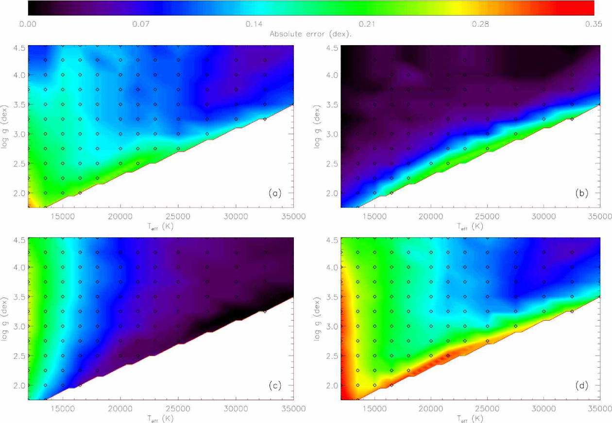
Figure 5: Contour maps displaying the effect of the errors in atmospheric parameters upon the derived abundances of the Mg ii 4481Å line at all points on the tlusty grid at a LMC metallicity calculated at a microturbulence of 5 km s^-1 for (a) an error in $T_{\rm eff}$ of 1 000 K, (b) an error in $\log g$ of 0.2 dex and (c) an error in $\xi$ of 3 km s^-1. Panel (d) shows the combined error calculated as the errors from (a), (b) and (c) summed in quadrature.

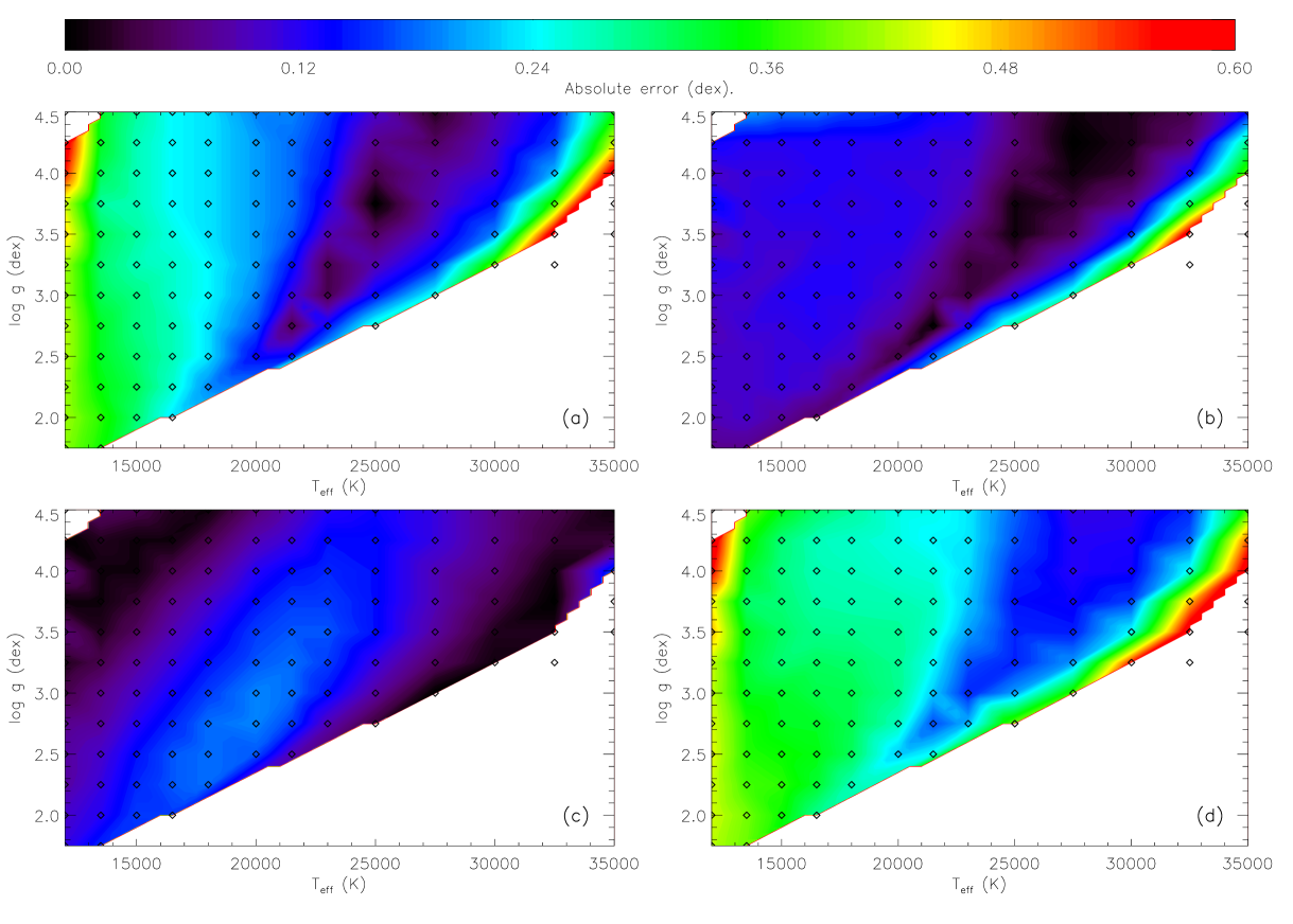
Figure 6: Contour maps displaying the effect of the errors in atmospheric parameters upon the derived abundances of the N ii 3995Å line at all points on the tlusty grid at a LMC metallicity calculated at a microturbulence of 5 km s^-1 for (a) an error in $T_{\rm eff}$ of 1 000 K, (b) an error in $\log g$ of 0.2 dex and (c) an error in $\xi$ of 3 km s^-1. Panel (d) shows the combined error calculated as the errors from (a), (b) and (c) summed in quadrature. Grid points for which the EW of the model line is less than 1 mÅ  have not been included in the contour mapping.

Table 10: Dependence of atmospheric parameters and abundances upon the assumed metallicity of a cluster for N 11-062.

	Metallicity Regime
	Galactic	LMC	SMC
$T_{\rm eff}$	30100	30400	31000
$\log g$	4.05	4.05	4.10
$\xi_{\rm Si}$	5	5	5
C ii	7.37	7.43	7.51
N ii	7.15	7.16	7.22
O ii	8.25	8.25	8.27
Mg ii	6.97	6.99	7.00
Si iii	7.16	7.16	7.21
Si iv	7.15	7.18	7.20

such we may have overestimated the actual error in the abundances from the adopted atmospheric parameters.

To illustrate how the errors given in Table 9 depend on atmospheric parameters at all points on our tlusty grid, in Fig. 5 and Fig 6 we plot the contribution of the uncertainty in each of the atmospheric parameters to the uncertainty in the derived photospheric abundances for two typical lines, Mg ii 4481Å and N ii 3995Å. These maps were calculated at LMC metallicity and at a microturbulence of 5 km s^-1. Of course it should be noted that the systematic errors will not affect each line of a particular species to the same extent, with for example, the predictions for a strong line being more dependent on the microturbulence estimate than for a weaker line. Figures. 7-31, only included online, show similar error contour maps for the following lines - C ii 4267Å, C iii 4647Å, N ii 3995Å, O ii 4075Å, O ii 4132Å, Si ii 4128Å, Si iii 4567Å and Si iv 4116Å- at Galactic, LMC and SMC metallicities.

In order to test the dependence of the atmospheric parameters and photospheric abundances upon the metallicity (iron content) adopted for the model atmosphere, we have analysed a single LMC target using both the Galactic and SMC grids and the resulting atmospheric parameters and abundances are given in Table 10. It can be seen that uncertainties in the atmospheric parameters arising from the metallicity adopted are well within those discussed in the above sections. Indeed, changing from one metallicity grid to another does not effect our derived microturbulence. The uncertainty in the abundances from the choice of metallicity grid is less than 0.1 dex for all species and less than 0.05 dex for O ii, Mg ii, Si iii and Si iv. This approach to estimating the error associated with the assumption of the base metallicity may be conservative in that, although the Fe abundance in any particular cluster may vary, it is unlikely to be as large as the +0.3 or -0.5 dex assumed above.

The derived Si abundance in each star is sensitive to the adopted atmospheric parameters, especially effective temperature and microturbulence. This is consistent with their use in estimating these parameters and is highlighted by the larger errors for the different species of silicon in Table 9. Additionally the spread of silicon abundances for stars in the same cluster is relatively large compared to that of the other species with the exception of nitrogen. The Si abundance should not be affected by chemical processing in the stellar interior (unlike nitrogen) and hence we would not expect to see this variation. Most of the error quoted in Table 9 arises from the uncertainty in microturbulence due to the Si iii lines being amongst the strongest observed in the spectra. To test if the spread in Si abundance estimates represents a real variation between stars in the same cluster or is an effect of microturbulence we have performed the following procedure. The average Si abundance of each cluster was calculated and then, holding $T_{\rm eff}$ and $\log g$ constant, the microturbulence was adjusted for every star so that the derived Si iii abundance from that star was the same as the cluster average. In Table 11 the adjusted microturbulence $\xi_{\rm av}$ and corresponding abundances for each species are listed. For comparison purposes the originally adopted miroturbulence $\xi_{\rm Si}$ is also given. For the majority of our sample the difference between $\xi_{\rm av}$ and $\xi_{\rm Si}$ is within our estimated error and the abundances given in Table 11 are generally within the uncertainties of those given in Table 9.

It is important to note that this procedure has not been possible for all stars. Two LMC stars, N 11-083 and N 11-124, have Si abundances lower than the cluster average. However they also have microturbulence values ($\xi_{\rm Si}$) of 0 km s^-1 and hence it is not possible to increase their stellar Si abundances. This problem also occurs in two SMC stars, NGC 346-029 and NGC 346-040. The abundances listed in Table 11 are therefore the same as those given in Table 9 for these four stars. NGC 346-043 has a microturbulence of 4 km s^-1 and even reducing the microturbulence to 0 km s^-1 does not increase the Si iii abundance to the cluster average and the estimates given in Table 11 are for a microturbulence of 0 km s^-1. Nevertheless, this procedure has been possible for the vast majority of our sample, and most of the cases where it fails are the problematic cases where a real value for the microturbulence cannot be determined from the Si lines. Although we no longer achieve ionization balance for several of the stars in our sample the different Si abundance estimates are consistent with an error of 1000 K in $T_{\rm eff}$. For NGC 6611, where we previously had the largest spread of Si abundances for stars in the same cluster, using the above procedure has eliminated both this spread and also noticeably improved the agreement of the other abundances. In the following sections we adopt the abundances listed in Table 11 but we note that our principle conclusions would be effectively unchanged if we had adopted the abundance estimates in Table 9.

Table 11: Absolute abundance estimates derived assuming the $T_{\rm eff}$ and $\log g$ given in Table 1 with the microturbulence adjusted in order to derive the same Si abundance for each star in each cluster where possible. The uncertainties are estimated by the same method as those in Table 9. The corrected carbon abundances (see Sect. 4.2) are given in brackets.

Star	$\xi_{\rm av}$	$\xi_{\rm Si}$	C II	N II	O II	Mg II	Si II	Si III	Si IV
NGC6611-006	8	7	7.85 $\pm$ 0.24 (7.96)	7.58 $\pm$ 0.12	8.50 $\pm$ 0.16	7.36 $\pm$ 0.22		7.41 $\pm$ 0.24	7.39 $\pm$ 0.30
NGC6611-012	5	6	7.92 $\pm$ 0.25 (8.26)	7.50 $\pm$ 0.24	8.55 $\pm$ 0.14	7.26 $\pm$ 0.23		7.45 $\pm$ 0.30	7.41 $\pm$ 0.51
NGC6611-021	0	0	7.82 $\pm$ 0.19 (7.99)	7.51 $\pm$ 0.11	8.60 $\pm$ 0.19	7.24 $\pm$ 0.22		7.40 $\pm$ 0.31	7.41 $\pm$ 0.52
NGC6611-030	1	5	8.09 $\pm$ 0.18 (8.26)	7.69 $\pm$ 0.21	8.57 $\pm$ 0.32	7.32 $\pm$ 0.25	7.34 $\pm$ 0.24	7.46 $\pm$ 0.32
NGC6611-033	4	1	7.99 $\pm$ 0.16 (8.16)	7.70 $\pm$ 0.12	8.54 $\pm$ 0.18	7.38 $\pm$ 0.19		7.43 $\pm$ 0.30	7.53 $\pm$ 0.50
N11-001	14	14	7.29 $\pm$ 0.16 (7.46)	8.20 $\pm$ 0.23	8.23 $\pm$ 0.30	7.12 $\pm$ 0.26	7.22 $\pm$ 0.27	7.20 $\pm$ 0.39	7.23 $\pm$ 0.72
N11-002	18	12	7.55 $\pm$ 0.16 (7.72)	8.00 $\pm$ 0.28	8.32 $\pm$ 0.40	7.07 $\pm$ 0.29	7.32 $\pm$ 0.28	7.18 $\pm$ 0.44
N11-003	13	13	7.34 $\pm$ 0.23 (7.68)	7.09 $\pm$ 0.26	8.34 $\pm$ 0.11	7.07 $\pm$ 0.24		7.17 $\pm$ 0.22	7.19 $\pm$ 0.60
N11-008	16	15	7.45 $\pm$ 0.09 (7.56)	7.84 $\pm$ 0.20	8.25 $\pm$ 0.16	7.12 $\pm$ 0.24		7.19 $\pm$ 0.25	7.15 $\pm$ 0.55
N11-009	17	17	7.55 $\pm$ 0.23 (7.72)	7.74 $\pm$ 0.30	8.38 $\pm$ 0.40	6.95 $\pm$ 0.25	7.18 $\pm$ 0.24	7.17 $\pm$ 0.41
N11-012	13	14	7.24 $\pm$ 0.26 (7.58)	7.71 $\pm$ 0.08	8.42 $\pm$ 0.18	7.02 $\pm$ 0.31		7.15 $\pm$ 0.30	7.14 $\pm$ 0.67
N11-014	12	13	7.60 $\pm$ 0.17 (7.77)	7.89 $\pm$ 0.19	8.27 $\pm$ 0.29	7.16 $\pm$ 0.25	7.14 $\pm$ 0.27	7.17 $\pm$ 0.40	6.76 $\pm$ 0.71
N11-015	11	11	7.45 $\pm$ 0.30 (7.79)	7.14 $\pm$ 0.30	8.36 $\pm$ 0.11	7.01 $\pm$ 0.30		7.21 $\pm$ 0.25	7.23 $\pm$ 0.62
N11-016	12	14	7.55 $\pm$ 0.25 (7.89)	7.90 $\pm$ 0.10	8.31 $\pm$ 0.18	7.27 $\pm$ 0.26		7.17 $\pm$ 0.30	7.15 $\pm$ 0.58
N11-017	16	17	7.51 $\pm$ 0.26 (7.85)	7.89 $\pm$ 0.28	8.33 $\pm$ 0.37	7.00 $\pm$ 0.25	7.14 $\pm$ 0.22	7.19 $\pm$ 0.39
N11-023	13	14	7.46 $\pm$ 0.21 (7.80)	7.16 $\pm$ 0.24	8.41 $\pm$ 0.17	7.00 $\pm$ 0.22		7.17 $\pm$ 0.25	7.18 $\pm$ 0.61
N11-024	12	12	7.48 $\pm$ 0.17 (7.65)	7.85 $\pm$ 0.10	8.32 $\pm$ 0.20	7.14 $\pm$ 0.23		7.15 $\pm$ 0.31	7.15 $\pm$ 0.58
N11-029	15	11	7.57 $\pm$ 0.39 (7.91)	7.10 $\pm$ 0.38	8.28 $\pm$ 0.31	6.93 $\pm$ 0.32		7.17 $\pm$ 0.36	6.93 $\pm$ 0.43
N11-036	11	11	7.32 $\pm$ 0.13 (7.49)	7.76 $\pm$ 0.12	8.33 $\pm$ 0.09	7.03 $\pm$ 0.20		7.17 $\pm$ 0.24	7.16 $\pm$ 0.59
N11-037	12	10	7.56 $\pm$ 0.20 (7.90)	$<$7.17 $\pm$ 0.23	8.18 $\pm$ 0.20	7.01 $\pm$ 0.13		7.18 $\pm$ 0.30	7.03 $\pm$ 0.44
N11-042	5	6	7.56 $\pm$ 0.21 (7.73)	6.92 $\pm$ 0.26	8.34 $\pm$ 0.18	7.00 $\pm$ 0.23		7.21 $\pm$ 0.24	7.32 $\pm$ 0.55
N11-047	8	8	7.67 $\pm$ 0.26 (8.01)	$<$6.88 $\pm$ 0.25	8.24 $\pm$ 0.16	7.00 $\pm$ 0.24		7.20 $\pm$ 0.22	7.19 $\pm$ 0.49
N11-054	10	11	7.52 $\pm$ 0.16 (7.69)	6.86 $\pm$ 0.13	8.45 $\pm$ 0.13	6.98 $\pm$ 0.21		7.16 $\pm$ 0.26	7.14 $\pm$ 0.60
N11-062	5	5	7.43 $\pm$ 0.22 (7.77)	7.16 $\pm$ 0.17	8.25 $\pm$ 0.14	6.99 $\pm$ 0.20		7.16 $\pm$ 0.22	7.18 $\pm$ 0.47
N11-069	11	10	7.62 $\pm$ 0.25 (7.96)	6.94 $\pm$ 0.22	8.44 $\pm$ 0.14	7.06 $\pm$ 0.24		7.18 $\pm$ 0.24	7.18 $\pm$ 0.56
N11-072	5	5	7.46 $\pm$ 0.14 (7.57)	7.38 $\pm$ 0.08	8.36 $\pm$ 0.15	7.12 $\pm$ 0.20		7.21 $\pm$ 0.24	7.21 $\pm$ 0.40
N11-075	5	3	7.52 $\pm$ 0.13 (7.86)	8.00 $\pm$ 0.25	8.18 $\pm$ 0.29	7.16 $\pm$ 0.17	7.23 $\pm$ 0.21	7.17 $\pm$ 0.37	7.23 $\pm$ 0.59
N11-083	-	0	7.53 $\pm$ 0.17 (7.70)	6.86 $\pm$ 0.20	8.33 $\pm$ 0.10	7.00 $\pm$ 0.19		7.06 $\pm$ 0.22	7.06 $\pm$ 0.45
N11-100	4	1	7.44 $\pm$ 0.23 (7.78)	7.62 $\pm$ 0.17	8.30 $\pm$ 0.10	7.10 $\pm$ 0.22		7.20 $\pm$ 0.23	7.19 $\pm$ 0.48
N11-101	8	8	7.74 $\pm$ 0.22 (8.08)	$<$7.09 $\pm$ 0.22	8.32 $\pm$ 0.12	7.21 $\pm$ 0.20		7.16 $\pm$ 0.17	7.17 $\pm$ 0.46
N11-106	5	7	7.50 $\pm$ 0.28 (7.84)	7.13 $\pm$ 0.28	8.35 $\pm$ 0.17	7.19 $\pm$ 0.24		7.19 $\pm$ 0.24	7.25 $\pm$ 0.34
N11-108	4	7	7.67 $\pm$ 0.30 (8.01)	7.21 $\pm$ 0.32	8.27 $\pm$ 0.20	7.14 $\pm$ 0.23		7.17 $\pm$ 0.25	7.43 $\pm$ 0.46
N11-109	10	14	7.41 $\pm$ 0.16 (7.58)	7.24 $\pm$ 0.23	8.32 $\pm$ 0.14	6.84 $\pm$ 0.20		7.18 $\pm$ 0.24	7.32 $\pm$ 0.58
N11-110	7	6	7.49 $\pm$ 0.18 (7.83)	7.39 $\pm$ 0.07	8.48 $\pm$ 0.25	7.06 $\pm$ 0.18		7.23 $\pm$ 0.32	7.28 $\pm$ 0.57
N11-124	-	0	7.56 $\pm$ 0.16 (7.90)	7.25 $\pm$ 0.17	8.12 $\pm$ 0.09	6.97 $\pm$ 0.15		6.94 $\pm$ 0.21	6.97 $\pm$ 0.43

Table 11: –continued

Star	$\xi_{\rm av}$	$\xi_{\rm Si}$	C II	N II	O II	Mg II	Si II	Si III	Si IV
NGC346-012	9	8	7.10 $\pm$ 0.08 (7.18)	6.93 $\pm$ 0.13	8.13 $\pm$ 0.08	6.70 $\pm$ 0.15		6.82 $\pm$ 0.16	6.85 $\pm$ 0.54
NGC346-021	3	1	7.36 $\pm$ 0.12 (7.45)	6.84 $\pm$ 0.11	8.16 $\pm$ 0.16	6.76 $\pm$ 0.15		6.78 $\pm$ 0.22	6.83 $\pm$ 0.48
NGC346-029	-	0	7.17 $\pm$ 0.29 (7.51)	$<$6.99 $\pm$ 0.29	8.02 $\pm$ 0.24	6.69 $\pm$ 0.21		6.69 $\pm$ 0.24	6.70 $\pm$ 0.39
NGC346-037	3	5	7.06 $\pm$ 0.12 (7.23)	7.55 $\pm$ 0.29	7.94 $\pm$ 0.39	6.62 $\pm$ 0.19	6.72 $\pm$ 0.18	6.79 $\pm$ 0.37
NGC346-039	3	0	7.32 $\pm$ 0.11 (7.40)	$<$6.59 $\pm$ 0.15	8.24 $\pm$ 0.12	6.73 $\pm$ 0.15		6.79 $\pm$ 0.22	6.84 $\pm$ 0.50
NGC346-040	-	0	7.11 $\pm$ 0.22 (7.45)	$<$6.88 $\pm$ 0.22	7.95 $\pm$ 0.15	6.39 $\pm$ 0.20		6.56 $\pm$ 0.19	6.57 $\pm$ 0.32
NGC346-043	-	4	7.21 $\pm$ 0.33 (7.55)	$<$6.75 $\pm$ 0.34	8.00 $\pm$ 0.22	6.83 $\pm$ 0.27		6.69 $\pm$ 0.23	6.78 $\pm$ 0.26
NGC346-044	4	0	7.27 $\pm$ 0.10 (7.44)	$<$6.94 $\pm$ 0.12	8.13 $\pm$ 0.27	6.66 $\pm$ 0.16		6.76 $\pm$ 0.30
NGC346-056	1	1	6.99 $\pm$ 0.25 (7.33)	7.40 $\pm$ 0.18	8.00 $\pm$ 0.26	6.81 $\pm$ 0.20		6.77 $\pm$ 0.25	6.74 $\pm$ 0.31
NGC346-062	6	12	7.15 $\pm$ 0.18 (7.49)	7.28 $\pm$ 0.11	7.91 $\pm$ 0.08	6.75 $\pm$ 0.17		6.82 $\pm$ 0.18	6.93 $\pm$ 0.36
NGC346-075	2	0	7.47 $\pm$ 0.12 (7.55)	$<$6.42 $\pm$ 0.15	8.03 $\pm$ 0.10	6.88 $\pm$ 0.15		6.79 $\pm$ 0.19	6.83 $\pm$ 0.41
NGC346-094	6	4	7.33 $\pm$ 0.13 (7.50)	7.34 $\pm$ 0.18	8.11 $\pm$ 0.10	6.75 $\pm$ 0.16		6.80 $\pm$ 0.19	6.78 $\pm$ 0.43
NGC346-103	1	0	7.02 $\pm$ 0.16 (7.36)	7.58 $\pm$ 0.13	7.96 $\pm$ 0.08	6.82 $\pm$ 0.16		6.80 $\pm$ 0.19	6.81 $\pm$ 0.35
NGC346-116	0	0	7.27 $\pm$ 0.10 (7.38)	6.93 $\pm$ 0.18	8.13 $\pm$ 0.09	6.70 $\pm$ 0.17		6.81 $\pm$ 0.20	6.81 $\pm$ 0.44

Table 12: Average abundances for NGC 6611, N 11 and NGC 346 from this analysis and CNO abundances from H ii regions in these clusters. The mean corrected carbon abundances are given in brackets. H ii region abundances are taken from Rodríguez (rod99 (1999)), Shaver et al. (sha83 (1983)) and Peña et al.(pen00 (2000)) for NGC 6611, Tsamis et al. (tsa03 (2003)) and Kurt & Dufour (kur98 (1998)) for N 11 and Kurt & Dufour (kur98 (1998)), Peimbert et al. (pei00 (2000)) and Shaver et al. (sha83 (1983)) for NGC 346. Errors in H ii region abundances are typically estimated to be 0.1-0.2 dex. Reyes (rey99 (1999)) estimate the SMC carbon abundace from several H ii regions to be 7.39 dex, see Sect. 5.2. Solar abundances are given for comparison and are taken from Asplund et al. (asp05 (2005)).

	NGC 6611		N 11		NGC 346		Solar
	This	H ii	This	H ii	This	H ii	Abundances
	Paper	Region	Paper	Region	Paper	Region
C	7.95 $\pm$ 0.11 (8.13)	8.23	7.48 $\pm$ 0.14 (7.73)	7.81	7.23 $\pm$ 0.15 (7.37)	7.17	8.39 $\pm$ 0.05
N	7.59 $\pm$ 0.10	7.64	7.54 $\pm$ 0.40	6.88	7.17 $\pm$ 0.29	6.50	7.78 $\pm$ 0.06
O	8.55 $\pm$ 0.04	8.56	8.33 $\pm$ 0.08	8.41	8.06 $\pm$ 0.10	8.11	8.66 $\pm$ 0.05
Mg	7.32 $\pm$ 0.06		7.06 $\pm$ 0.09		6.74 $\pm$ 0.07		7.53 $\pm$ 0.09
Si	7.41 $\pm$ 0.05		7.19 $\pm$ 0.07		6.79 $\pm$ 0.05		7.51 $\pm$ 0.04

3.7.2 Correlations of abundances with atmospheric parameters

We have searched for any dependence in our abundances with the stellar atmospheric abundances for the Magellanic Cloud clusters using the values given in both Tables 9 and 11. For carbon, oxygen, magnesium and silicon there is no evidence of any significant correlation. For example, in N 11 a linear least squares fit suggests that the oxygen abundance decreases by less than 0.1 dex over a range in gravity from 2.0 dex to 4.5 dex, while the 2$\sigma$ errors are greater than the gradients in all cases. Additionally, if we adopt the abundances given in Table 11 and do not include the stars where we where unable to determine $\xi_{\rm av}$, the gradients of the best-fitting lines in the majority of cases are less than their 1$\sigma$ errors. We have not investigated any dependence of the nitrogen abundance with the atmospheric parameters due to the scatter in the nitrogen abundances and also because we expect to see a correlation with surface gravity due to evolutionary effects (see Sect. 6.4).

4 Chemical composition of the three clusters

In Table 12, the average C, N, O, Mg and Si abundances for each cluster are presented. These averages have been calculated from the stellar abundances listed in Table 11 and are weighted by the quoted uncertainties. The Si abundances are the weighted average of the Si ii, Si iii and Si iv abundances. The five stars without a $\xi_{\rm av}$ value in Table 11 have not been included in the estimate of these averages (see Sect. 3.7.1) nor are upper limits to the nitrogen abundance included in the nitrogen average. The quoted errors are the 1$\sigma$ standard deviation in abundances derived from each star analysed in the cluster.

4.1 Helium

In our analysis we have not explicitly derived helium abundances but instead have assumed a nominal value (11.0 dex) throughout. To test the validity of this assumption we have fitted theoretical models at the appropriate atmospheric parameters to the observed He i line at 4026Å. It should be noted that due to the strength of this line the theoretical profiles are dependent on the adopted microturbulence. Other weaker He lines are available, such as the 4169Å and the 4437Å lines but these lines are not well observed in all of our spectra. Within the uncertainties in our atmospheric parameters we find excellent agreement between theory and observation for the majority of stars in our sample. In Fig. 32 we show the quality of the fit for two SMC objects, NGC 346-075 and NGC 346-103, which have the lowest and highest estimated SMC nitrogen abundance estimates respectively.

Figure 32: Fits of model spectra with a He abundance of 11.0 dex (smooth curve) to the observed He i 4026Å line in NGC 346-075 and NGC 346-103, upper and lower plots respectively. These objects have nitrogen abundances which differ by over 1.0 dex.

The few cases where discrepancies are found are all supergiant stars having relatively large values of microturbulence. In these cases the discrepancy can be attributed to the senstivity of the theoretical profiles to this parameter and indeed the weaker He lines (where available) are in excellent agreement with theory. As such, within the uncertainties in the atmospheric parameters, we believe that we are justified in assuming normal helium abundances throughout our analysis but small variations cannot be ruled out.

4.2 Carbon

In Tables 9 and 11, the carbon abundances have been determined solely from C ii lines, despite the spectra of our hotter targets containing measurable C iii lines. The latter have not been included in our abundance analysis because our tlusty model grid used a relatively simple C iii ion. Our choice of model ions was discussed in Dufton et al. (duf05 (2005)) and the models were obtained from Lanz & Hubeny (lan03 (2003)) and Allende-Prieto et al. (all03 (2003)). Although a grid including a more sophisticated C iii ion could have been generated, this was not considered worthwhile given the relatively few stars containing C iii lines.

In previous studies (Sigut sig96 (1996) and Lennon et al. len03 (2003)) it has been found that estimates of the carbon abundance from the C ii line at 4267Å gives lower abundances than estimates from other C ii lines. Recently, Nieva & Przybilla (nie06 (2006)) have constructed a comprehensive C ii non-LTE model ion which removes this discrepancy. However, given the relatively simple model ion used in our tlusty code, we have adopted the correction of +0.34 dex reported by Lennon et al. (len03 (2003)) to the abundances estimated from the 4267Å line. Indeed, as discussed in Sect. 5.2 this improves the agreement of our stellar carbon abundances with previous interstellar studies. Both uncorrected and corrected carbon abundances are given in Tables 11 and 12, with the error estimates for the latter being either identical or similar to those for the uncorrected values.

4.3 Nitrogen

In several stars, especially at the lowest metallicity studied, it was not possible to observe any nitrogen lines. In these cases an upper limit to the EW of the nitrogen line at 3995Å was estimated by adding a Gaussian profile (with the same width as the other observed metal absorption lines) to the spectra. The strength of the Gaussian was then varied until it became obvious in the spectral noise. The size of the apparent absorption line was then measured and the resulting EW was taken as an upper limit to the EW of a nitrogen line. This upper limit was then used to derive an upper limit to the nitrogen abundance in the star.

In the spectra where we observe more than one nitrogen line the derived nitrogen abundances of each line agree well. However, there is a very large spread in the nitrogen abundance between stars in each of the Magellanic Cloud clusters that is not replicated in our NGC 6611 sample. As discussed in Sect. 6.4, we believe that this is due to evolutionary effects during the stellar lifetimes and is not seen in NGC 6611 due to its higher metallicity and lack of supergiant targets.

4.4 Oxygen

As can be seen from Table 11 the oxygen abundances derived for individual stars in each of the three clusters are in good agreement. This suggests that the oxygen abundance is effectively constant within each cluster or at least, any variations being too small to be detected. It should be noted that as seen in Fig. 4 there is quite a large spread between the oxygen abundance derived from different absorption lines of the same star. We believe that these differences are due to uncertainties in the atomic data and the theoretical calculations, but given the large number of oxygen lines observed, the mean oxygen abundances should be robust.

4.5 Magnesium

The magnesium abundances are based solely upon the 4481Å line and very good agreement between the estimates for stars in the same cluster is seen. This agreement is encouraging as we do not expect to see variations in Mg as it should be unaffected by the nucleosynthetic processes that affect our CNO abundances.

4.6 Silicon

As discussed above the Si abundances are especially dependent on the adopted atmospheric parameters and hence we base the parameters upon these lines. Because of the methodology the Si abundances given in Table 11 are essentially constant. Nevertheless, from Table 9 it can be seen that the majority of the uncorrected Si abundances in each cluster are in good agreement within the uncertainties.

5 Comparisons with previous work

5.1 Stellar studies

5.1.1 NGC6611

Table 13: Comparison of NGC 6611 stars with those analysed by Kilian-Montenbruck et al. (kil94 (1994)) (Kil94), who have used non-LTE line formation calculations with LTE models.

	NGC 6611-006		NGC 6611-012		NGC 6611-021		NGC 6611-033
	This	Kil94	This	Kil94	This	Kil94	This	Kil94
	Paper		Paper		Paper		Paper
$T_{\rm eff}$ (K)	31250	32600	27200	29400	26250	29400	25600	28600
$logg$ (dex)	4.00	4.17	3.90	4.17	4.25	4.39	4.00	4.21
$\xi$ (km s -1)	8	8	5	10	0	0	4	5
$v\sin i$ (km s -1)	20	29	95	86	30	38	25	41
Carbon	7.85	8.28	7.92	8.23	7.82	8.23	7.99	8.41
Nitrogen	7.58	7.78	7.50	7.72	7.51	7.89	7.70	8.02
Oxygen	8.50	8.69	8.55	8.39	8.60	8.62	8.54	8.52
Magnesium	7.36	7.21	7.26	7.39	7.24	7.32	7.38	7.51
Silicon	7.41	7.63	7.45	7.11	7.40	7.21	7.43	7.01

Four of the five stars analysed in NGC 6611 have previously been analysed by Kilian-Montenbruck et al. (kil94 (1994)) and in Table 13 the two analyses are compared. It can been seen that Kilian-Montenbruck et al. derive systematically higher effective temperatures and hence higher gravities, which may be due to their adoption of LTE models with only partial line blanketing. In one case, NGC 6611-021, this difference is over 3 000 K. Although our tlusty model predicts that the He ii lines would be present at this higher temperature, they would probably be hidden by the noise in the observational spectra and hence cannot be used to constrain the temperature estimate. However, the predicted Si iv line at 4116Å would be 50% stronger at this higher temperature and a change of this magnitude would be incompatible with the observed spectra. Although there are some differences between the derived abundances, given the differences in the atmospheric parameters, these are not significant. Additionally we note that the scatter in abundances derived here is less than that previously seen. For example we see a range of less than 0.1 dex in our oxygen abundance compared with a range of 0.3 dex in the O abundances of Kilian-Montenbruck et al. As we have used both non-LTE line formation calculations and non-LTE models (rather than LTE models adopted by Kilian-Montenbruck et al.), we believe the results presented here are an improvement on those currently available in the literature.

5.1.2 N11

A search of the literature revealed that only one of our N 11 target stars had previously been analysed, N 11-100, by Rolleston et al. (rol02 (2002)). In Table 14 we present a comparision of the two analyses. Given that Rolleston et al. adopted LTE techinques, the atmospheric parameters compare well and the abundances differ by at most 0.3 dex between the two analyses.

5.1.3 NGC346

Two stars in NGC 346 have previously been analysed, viz. NGC 346-029 by Rolleston et al. (rol93 (1993)) and NGC 346-043 by Hunter et al. (hun05 (2005)). In Table 15 we present a comparision of the two analyses. We find good agreement between our analysis of NGC 346-029 and that of Rolleston et al., who used LTE methods and observational data with a S/N ratio of 35, compared to a S/N ratio of 140 for the FLAMES data. Hunter et al. have used effectively the same methods as discussed here to analyse UVES spectra of NGC 346-043 and the agreement between the two analyses is encouraging, with all the parameters and abundance estimates consistent within the uncertainties.

Table 14: Comparison of our derived parameters and abundances of N 11-100 with those derived by Rolleston et al. (rol02 (2002)) (R02).

	N 11-100
	This	R02
	Paper
$T_{\rm eff}$ (K)	29700	29500
$logg$ (dex)	4.15	4.10
$\xi$ (km s -1)	4	6
$v\sin i$ (km s -1)	30	30
Carbon	7.44	$<$7.64
Nitrogen	7.62	7.86
Oxygen	8.30	8.28
Magnesium	7.10	6.81
Silicon	7.20	7.21

Table 15: Comparison of our derived parameters and abundances for NGC 346-029 and NGC 346-043 with those estimated by Rolleston et al. (rol93 (1993)) (R93) and Hunter et al. (hun05 (2005)) (H05) respectively. Note that the abundances given in this table are from Table 9 rather than Table 11 as the method of adjusting the microturbulence to derive the average Si cluster abundance for these stars was not possible, see Sect.3.7.1.

	NGC 346-029		NGC 346-043
	This	R93	This	H05
	Paper		Paper
$T_{\rm eff}$ (K)	32150	30500	33000	32500
$logg$ (dex)	4.10	4.0	4.25	4.25
$\xi$ (km s -1)	0	5	4	5
$v\sin i$ (km s -1)	25	28	10	8
Carbon	7.17	6.80	7.24	7.45
Nitrogen	6.99	$<$7.20	$<$6.73	$<$6.73
Oxygen	8.02	8.00	7.97	7.82
Magnesium	6.69	7.10	6.81	6.77
Silicon	6.69	6.50	6.56	6.42

5.1.4 Other stellar studies

Venn (ven99 (1999)) has obtained SMC abundances from A-type supergiants and these are generally in good agreement with the NGC 346 abundances presented here. Venn also observed a similar variation of the nitrogen abundances from different stars. Additionally Dufton et al. (duf05 (2005)), Trundle & Lennon (tru05 (2005)) and Trundle et al. (tru04 (2004)) have determined chemical abundances for approximately 30 SMC supergiants. Their C, O, Mg and Si abundances are in excellent agreement (within 0.1 dex) with those presented in Table 12. They report higher N abundances than those derived here but this may be due to the more evolved nature of their sample compared to that presented here. Bouret et al. (bou03 (2003)) and Heap et al. (hea06 (2006)) have derived abundances from SMC O-type stars. Their O and Si abundances are in excellent agreement with those in Table 12 while they find a similar spread in the nitrogen abundances. Their average C abundance is 0.2 dex higher than that given in Table 12 but given the uncertainties in our estimate this is unlikely to be significant. In Sect. 6.4, we discuss further the implications of these studies for stellar evolutionary models.

Korn et al. (kor05 (2005)) have obtained LMC abundances from targets in NGC 2004 and the abundances which we derive for N 11 are within their uncertainties for all elements except carbon. As discussed in Sect. 4.2 this may be at least partially due to problems with our derived carbon abundances.

5.2 H ii regions

In Table 12 we present CNO abundances for the H ii regions NGC 6611, N 11 and NGC 346 taken from the literature. Unfortunately it was not possible to find one source which covered all three clusters and so the abundance estimates utilise a variety of methods.

It is particularly difficult to obtain carbon abundances from these H ii regions and we have found only one recent reference for each cluster. This is primarily due to the high quality UV spectra that is required. In the case of both NGC 6611 and N 11 our uncorrected carbon abundances are $\sim$0.3 dex lower than those found from the H ii region analyses, whilst our corrected values are in excellent agreement with those from H ii region studies. However, we find poorer agreement between the corrected carbon abundance of NGC 346 and that from Kurt & Dufour (kur98 (1998)) compared to the uncorrected value, although within the uncertainties this may not be significant. For example, Reyes (rey99 (1999)) find that the average carbon abundance derived from five different H ii regions in the SMC is 7.39 dex (compared with 7.20 dex from Kurt & Dufour), which is in excellent agreement with our corrected value.

Our estimated nitrogen abundance from B-type stars in NGC 6611 is in excellent agreement with those from H ii regions, in contrast to N 11 and NGC 346 where our average nitrogen abundances are higher than those given in Table 12. However as discussed in Sect. 4.3 we see a very large spread in the nitrogen abundances between stars in the same cluster and we believe that this is due to chemical processing in the stellar interior and not due to any inconsistency in our analysis. For the stars with the lowest nitrogen abundance estimates in each cluster, there is excellent agreement with H ii region results.

The average oxygen abundances in each cluster estimated from our sample are in excellent agreement with the averages of the H ii region oxygen abundances given in Table 12. This is expected as, given the relatively large oxygen abundance in these clusters, any small changes due to mixing of nucleosynthetic processed material to the surface would be difficult to detect.

6 Discussion

6.1 Atmospheric parameters and abundances

Atmospheric parameters and abundances have been presented for approximately 50 narrow lined B-type stars covering three metallicity regions, Galactic, LMC and SMC. To date, this is the most extensive abundance analysis of these regions using a consistent method of analysis. Also, the uncertainties in our estimated abundances have been fully quantified to take into account the errors in the atmospheric parameters. Although we determine projected rotational velocities it is not possible for us to examine these distributions as a function of metallicity due to the selection effects that we have used. In a future paper we intend to derive atmospheric parameters and $v\sin i$ values for all the LMC and SMC stars observed in the FLAMES survey using similar methods to those described in Dufton et al. (duf06 (2006)).

6.2 Abundance ratios

In Table 16 the ratios of the Magellanic Cloud cluster abundances to the Galactic cluster abundances are presented. Excluding nitrogen, the abundances in the LMC cluster are on average 0.3 dex lower than those in the Galactic cluster, and the SMC abundances are on average 0.6 dex lower than the Galactic case which is in good agreement with the iron abundances adopted in our model atmosphere grids (Sect. 3.1). However, there is some spread in these values. For example, oxygen appears to be the least depleted element in both the LMC and SMC cluster and nitrogen is the most depleted.

In Table 16 we also present the ratios for CNO as derived from the H ii region results given in Table 12. It can be seen, in the majority of cases, that these are in excellent agreement with those derived in this analysis. The only exception being the carbon NGC 346/NGC 6611 ratio, although as discussed earlier this may be due to choice of H ii region analysis. Adopting the H ii region carbon abundance from SMC analysis of Reyes (rey99 (1999)) (see Sect. 5.2) results in a ratio of -0.86 dex which is in better agreement with that derived from our stellar analysis. Slightly greater depletions of carbon than for other elements (except nitrogen) are evident and this has previously been observed by Dufour et al. (duf82 (1982)) from H ii region analyses. We also note the relatively small oxygen underabundances implied by the H ii region studies, which are consistent with our stellar results.

Table 16: Logarithmic ratios of abundances derived from the Magellanic Cloud clusters to those derived from the Galactic cluster. Note that the ratios for nitrogen use the lowest nitrogen abundance we derive from the Magellanic Cloud cluster stars rather than the average nitrogen given in Table 12. Additionally the ratios for the carbon abundance use the corrected abundance estimates (compare with ratios of -0.47 and -0.72 for N 11/NGC 6611 and NGC 346/NGC 6611 respectively from the uncorrected values). The ratios derived from the H ii region abundances in Table 12 are also given.

	N 11/NGC 6611		NGC 346/NGC 6611
	This	H ii	This	H ii
	Paper	Regions	Paper	Regions
C	-0.40 $\pm$ 0.17	-0.42	-0.76 $\pm$ 0.19	-1.10
N	-0.73 $\pm$ 0.18	-0.77	-1.17 $\pm$ 0.18	-1.14
O	-0.22 $\pm$ 0.09	-0.15	-0.49 $\pm$ 0.11	-0.45
Mg	-0.26 $\pm$ 0.11		-0.58 $\pm$ 0.09
Si	-0.22 $\pm$ 0.09		-0.62 $\pm$ 0.07

6.3 Temperature scales of B-type stars

Figure 33: Temperature scales derived from the atmospheric parameters given in Table 1 for each cluster, plots (a), (b) and (c). The solid points represent stars with $\log g$ $\geq$ 3.70 dex and open circles represent stars with $\log g$ $<$ 3.70 dex. The dotted and dashed lines are the temperature scales derived from the O-star analysis of Massey et al. (mas05 (2005)) for luminosity class V & III stars and luminosity class I stars respectively. In (d) we compare the temperature scales from the three clusters for stars with $\log g$ values $\geq$ 3.70 dex and the solid, long-dashed and short-dashed lines represent the best-fitting lines for the NGC 6611, N 11 and NGC 346 stars, respectively. Note that NGC 6611-006 is not included in plots (a) and (d) due to the uncertainty in its spectral type, see footnote in Table 1.

In previous studies, see for example Voels et al. (voe89 (1989)) and Massey et al. (mas05 (2005)), it has been reported that there is a significant difference in temperature scales between different luminosity class stars at the same metallicity and also for stars of the same spectral type at different metallicities. In Figs. 33 (a), (b) and (c) plots of spectral type against $T_{\rm eff}$ for all the stars in Table 1 are presented for NGC 6611, N 11 and NGC 346 respectively. From Figs. 33 (b) and (c) it can be seen that the temperature derived from the lower gravity stars in the LMC and SMC clusters are smaller than those from higher gravity stars. Unfortunately for NGC 6611 we have no stars with $\log g$ $<$ 3.70 dex. However, Crowther et al. (cro05 (2005)) have derived atmospheric parameters for Galactic B-type supergiants and a comparison with our results shows again that the lower gravity stars have lower temperatures for a given spectral type. This is in contrast to the temperature scale derived by Massey et al. for O-stars who have previously reported that while the temperature of early O-type stars can be higher by up to 6 000 K for main-sequence compared to supergiant stars, the difference decreases as one moves towards later O-types with no significant difference by B0. However we note that they had only three stars in their SMC sample (two giants and one supergiant) and no stars in their LMC sample are later than O8. Additionally, in deriving temperature scales, Massey et al. group together giant and main-squence stars as they find little difference between the gravity estimates for these luminosity classes. However, their two SMC giant stars later than O8 have gravities of 3.27 and 3.52 dex and hence may not be representative of the main-sequence temperature scale for late type O stars. In Figs. 33 (a), (b) and (c) the dotted and dashed lines represent the temperature scales from the O-star analysis of Massey et al. for luminosity class V & III stars and luminosity class I stars respectively.

In Fig. 33 (d) we compare the temperature scale for the (near) main-sequence B-type stars at Galactic, LMC and SMC metallicities. Although there are relatively few data points covering only a small range in spectral type there appears to be a trend of increasing temperature as one moves towards lower metallicities for stars of the same spectral type. Massey et al. (mas05 (2005)) report the same effect for both high and low gravity early O-type stars although they find little difference by B0. In contrast we see a difference of 2000 K between dwarf stars in the SMC and dwarf stars in the Galaxy. Mokiem et al. (2006a ) also report a similar effect for their O and early B-type stars with the temperature scale derived from their SMC stars being in good agreement with that shown in Fig. 33 (d). At present we are unable to undertake a detailed comparison of the temperature scale for low gravity stars due to a lack of giants and supergiants in our Galactic sample.

6.4 Evolutionary effects

(a)

Figure 34: Hertzsprung-Russell diagrams for NGC 6611 (a), N 11 (b) and NGC 346 (c). The size of the symbols represent the absolute nitrogen abundances. Open symbols represent upper limits to the nitrogen abundances. Squares and circles represent potential binaries and single stars respectively. Evolutionary tracks have been obtained from Meynet et al. (mey94 (1994)), Schaller et al. (sch92 (1992)), Schaerer et al. (sch93 (1993)), and Charbonnel et al. (cha93 (1993)). Isochrones have been calculated from Meynet et al. (mey93 (1993)). In panel (b) stars 100 and 101 overlap.

(b)

(c)

Figure 34: –continued

Nitrogen is often used as a probe of the evolutionary history of B-type stars due to its initial low abundance, especially in the Magellanic Clouds, (see, for example, Lennon et al. len03 (2003), Venn ven99 (1999) and Gies & Lambert gie92 (1992)). Observed surface enrichments and depletions arise from processes which mix core processed material to the photosphere and hence the observed surface abundances can trace evolutionary effects such as rotational mixing, mass-loss and binarity. In this section the evolutionary status of the objects in this sample is discussed and compared with current theoretical models where possible. Carbon depletions can also be used as a probe of evolutionary history but given its initial high abundance (compared with nitrogen) it is difficult to detect small abundance variations. For example, assuming that the sum of the carbon and nitrogen nuclei are conserved, the uncertainities in the carbon abundance estimates appear to mask any evolutionary effects for the majority of objects. Additionally, no convincing anti-correlation between the carbon and nitrogen abundances is observed, hence the former are not discussed in this section.

Figure 34 displays Hertzsprung-Russell (HR) diagrams of our target stars. The absolute nitrogen abundance is indicated by the size of the symbol, open symbols represent upper limits to the nitrogen abundance and square symbols represent stars where radial velocity variations (potential binary systems) have been detected, see Sect. 2.2. From Evans et al. (eva05b (2006)) it is evident that we sample both cluster and field stars and hence the isochrones shown in Fig. 34 are for information only as the populations are unlikely to be coeval.

We sample only five main-sequence NGC 6611 stars and these objects have very similar nitrogen abundances and are in good agreement with the nitrogen abundance estimated from H ii regions. Given the lower baseline nitrogen abundance of N 11 and NGC 346 it is easier to detect small nitrogen enhancements. For example, if we add the average nitrogen enrichments observed in the main-sequence objects of N 11 and NGC 346 to the base-line nitrogen abundance of NGC 6611 (by number) we obtain enrichments of only 0.10 and 0.12 dex which is consistent with the scatter seen in the nitrogen abundances of our Galactic sample. Hence we limit our following discussion to the Magellanic Cloud objects.

From Fig. 34 (b) and (c) it is immediately apparent that in both the LMC and SMC samples, nitrogen variations of over 1.0 dex are seen. These variations are present even for the main-sequence objects, with a spread of 0.7 in N 11 and 1.1 dex in NGC 346. For the more evolved objects a range of nitrogen enhancements is also evident. In NGC 346 the evolved objects do not appear to have systematically higher nitrogen enhancements compared to those on the main-sequence, although the numbers of evolved objects are limited. Additionally in N 11 there are non-main-sequence objects with close to baseline nitrogen abundances, for example N 11-054, and yet there are also giant objects (such as N 11-036) showing significant nitrogen enhancement.

In Fig. 35 and Fig. 36 the nitrogen abundance as a function of $\log g$ is plotted for the LMC and SMC samples (divided into those targets with masses less than and greater than 20M_☉) respectively. Given the smaller sample size of NGC 346 and also that all our objects have masses $<$20M_☉, to make a direct comparison with the N 11 sample we have included other published results for SMC B-type supergiants (see Fig. 36 caption for details). Additionally Venn (ven99 (1999)) has analysed several AF-type supergiants in the SMC and these objects are plotted left of the dotted line in Fig. 36 using updated nitrogen abundances from Venn & Przybilla (ven03 (2003)). Unfortunately, due to a lack of other analyses in the LMC it is not possible to compare our N 11 sample with similar objects.

Histograms of the stellar nitrogen abundances have also been plotted in Fig. 37 and Fig. 38. Objects for which only upper limits to the nitrogen abundance have been derived are included as dashed lines on these plots. The dotted line indicates the position of the baseline nitrogen abundance of each of the Magellanic Clouds (see Sect. 7).

In Sect. 6.4.1 and Sect. 6.4.2 we now discuss the observed nitrogen enhancements for LMC and SMC samples respectively. In particular, the observational evidence for rotational mixing, blue loops, mass-loss and binarity is discussed and compared with theoretical predictions, where possible, in each metallicity regime.

6.4.1 LMC

(a)

(b)

Figure 35: Variation of the N 11 stars as a function of $\log g$. Open symbols represent stars with upper limits to their nitrogen abundance. Symbols which have been circled represent stars for which we see evidence of binarity. Stars with evolutionary masses $<$20M_☉ and $\geq$20M_☉ are plotted in (a) and (b) respectively.

(a)

(b)

Figure 36: Variation of the NGC 346 stars as a function of $\log g$. Symbols are equivalent with those in Fig. 35. In addition to the B-type stars analysed in this sample, SMC B supergiants and giants (Dufton et al. duf05 (2005), Trundle et al. tru04 (2004), Trundle & Lennon tru05 (2005) and Lennon et al. len03 (2003)) and AF supergiants (Venn ven99 (1999) updated with N abundances from Venn & Przybilla ven03 (2003)) have also been plotted for comparison. Points left of the dotted line are AF stars, points to the right are B type stars. The stars analysed in this analysis are labelled.

Figure 37: Histograms showing the spread the in nitrogen abundances of the N 11 stars. The dashed line represents upper limits to the abundance. The dotted lined indicates the baseline nitrogen abundance of the LMC. Similarly to Fig. 35 the stars are split by mass.

Both Fig. 35 and Fig. 37 show that significant nitrogen enhancement can occur during the main-sequence lifetime. The most evolved objects in the sample appear to be further enhanced in nitrogen than the main-sequence objects and there is some evidence of a bi-modal distribution. However, there are some Ia supergiants with low nitrogen abundances, for example, N 11-003 which has a nitrogen abundance 0.5 dex lower than the most enhanced main-sequence object.

Rotational mixing of core processed material into the stellar photosphere can increase the photospheric nitrogen abundance and the variable nitrogen abundances that are observed can be interpreted as being due to different rotation rates. Lamers et al. (lam01 (2001)) have calculated, for LMC metallicity, the N/O ratio that would be expected by the end of the main-sequence due to rotation, as a function of the ratio of the mixing time to the main-sequence lifetime for masses of 85, 40, 60 and 20M_☉. For their longest mixing times (where the mixing time to main-sequence lifetime ratio is 5), a nitrogen abundance of approximately 8.0 dex (scaled by the oxygen abundance that we determined here) would be expected by the end of the main-sequence for an initial mass of 20M_☉. This is significantly greater than the nitrogen abundances of our objects with such masses. Although not all of our LMC objects are at the end of the main-sequence, the majority of rotational mixing is thought to occur early in the main-sequence lifetime where rotational rates are highest (Maeder & Meynet mae01 (2001)) and hence this may indicate that longer mixing times or less efficient mixing needs to be considered.

A possible explanation for the high nitrogen abundances derived for several of our higher mass evolved objects in N 11 is that these stars are on blue loops and the enhancement arises from convective mixing during the red supergiant phase. Indeed this was the scenario that was invoked to explain the apparently high nitrogen abundance of the progenitor to the LMC supernova 1987A (N/O=1.6$\pm$0.8 dex, Fransson et al. fra89 (1989)). Lamers et al. (lam01 (2001)) have used the evolutionary tracks of Meynet et al. (mey94 (1994)) to predict the N/O ratio that would be expected after convective mixing in the red supergiant phase as a function of the remaining fraction of the mass of the star at the onset of outer convection, but they do not include any rotational mixing in this calculation. For negligible mass-loss at an inital mass of 20M_☉ their predicted N/O abundance ratio is approximately 0.5, which again equates to a nitrogen abundance of approximately 8.0 dex. Although the majority of the N 11 supergiants have nitrogen abundances of less than 8.0 dex, within the uncertainties this is a viable explanation for many of the high nitrogen objects in this sample. However, inspection of Fig. 34(b) shows that although blue loops are indeed predicted for several of the low mass evolutionary tracks, they do not extend far enough into the blue or to high enough masses to encompass the objects in this sample. Additionally, given that the Lamers et al. (lam01 (2001)) predictions of the nitrogen abundance from both rotational mixing (at 20M_☉ for their longest mixing time) and convective mixing during the red-supergiant phase (at 20M_☉ with no mass-loss) are both 8.0 dex it is difficult to distinguish these processes.

Mass-loss in massive stars can affect the observed abundances as the outer layers of the star are removed and the more mixed inner layers are revealed. More massive stars generally have higher mass-loss rates. However we note that in both Fig. 35 and Fig. 37 there is little evidence for a trend of increasing nitrogen enhancement with increasing mass, although the majority of the sample covers a small range in mass.

In Fig. 35 objects for which radial velocity variations have been detected are circled. The circled main-sequence objects typically have radial velocity variations on the order of 10-40 km s^-1 and are likely to be binary systems. These objects have near-normal nitrogen abundances and within the uncertainties these are similar to those stars where we have not detected evidence of binarity. The evolved radial velocity variable objects in the sample are all significantly enhanced in nitrogen. It is worth emphasizing that several of the high nitrogen objects in N 11 were observed with UVES and as only a single observation was available it was not possible to examine these objects for velocity variations and so there may be more radial velocity variable objects than shown in Fig. 35. Additionally three of the four evolved velocity variable objects have detected velocity shifts of less than 5 km s^-1 and binarity may not be the only explanation (see Sect. 2.2).

However, if these objects are in binary systems they may have undergone a mass-transfer process from which we would expect to see an enhancement of nitrogen, although at present there are no detailed theoretical predictions of abundances in post mass-transfer LMC binary systems. Wellstein et al. (wel01 (2001)) calculate the masses and orbital parameters of post mass-transfer contact-free binary systems where the remnants are O- and early B-type stars with a helium star companion. These systems are generally long period systems (greater then 60 days) and the primary objects have orbital velocities of less than 20 km s^-1. Given the time coverage of our N 11 observations (those of the 6515Å region were separated by 35 days) and random angles of inclination the velocities shifts of a few km s^-1 which we detect for the most evolved objects may be compatible with the predictions of Wellstein et al. and so the high nitrogen abundance could be due to mass-transfer. Wellstein et al. calculate nitrogen enhancement factors of 5.4 and 4.0 for a representative Case A (mass-transfer during core hydrogen burning) and Case B (mass-transfer during core helium burning) binary scenario. However as these calculations are at solar metallicity it is difficult to directly compare them with our LMC abundances. Follow-up observations of these objects are necessary in order to determine if these objects truly are binary systems and if so to obtain accurate orbital parameters to compare with the predictions of Wellstein et al. It is also important to note that the nitrogen enhancements in these systems are similar to the apparently single objects and hence it may not be necessary to invoke binarity to explain the observed abundances.

6.4.2 SMC

Figure 38: Histograms showing the spread in the nitrogen abundances of the NGC 346 stars. The dashed line represents upper limits to the abundance. The dotted lined indicates the baseline nitrogen abundance of the SMC. Similarly to Fig. 36 the stars are split by mass. For comparison SMC O type stars (Heap et al. hea06 (2006), Evans et al.eva04 (2004) and Crowther et al. cro02 (2002)), AF supergiants and additional B supergiants and giants are included (see references in Fig. 36).

Both Fig. 36 and Fig. 38 show that significant nitrogen enhancement occurs on the SMC main-sequence. As in the LMC sample it appears that the more evolved stars can have higher enhancements than that observed on the main-sequence and the most massive stars can have higher nitrogen enhancements than their less massive counterparts. Indeed the similarlity of Fig. 36(a) and Fig. 35(a), when the offset due to baseline nitrogen abundance is accounted for, is remarkable and probably shows that the LMC and SMC stars go through similar evolutionary processes. This appears to suggest that the maximum N abundance detected in both the LMC and SMC are independent of metallicity, but we should caution that the SMC objects with the highest nitrogen abundances have been obtained from the literature and hence differences in methodology must be considered. The A-supergiants in Fig. 36(a) have similar, although slightly higher, enhancements to the main-sequence objects again indicating that a significant proportion of enhancement occurs during the main-sequence lifetime. Comparison of Fig. 36(a) and (b) shows that on the main-sequence a nitrogen enhancement of typically 1.0 dex occurs while after the main-sequence an additional 0.4 dex of enhancement may occur. However, it is important to note that it is necessary to add only 7.56 dex of material to a baseline abundance of 6.5 dex to be able to achieve an abundance of 7.6 dex, yet it takes a further 7.78 dex of material to increase the observed nitrogen abundance from 7.6 dex to 8.0 dex. This highlights the importance of studying low metallicity environments in order to observe small amounts of mixing.

Various degrees of rotational mixing on the main-sequence can again explain the variation of nitrogen abundances. In Fig. 39 the nitrogen abundance of our NGC 346 sample of stars is plotted as a function of luminosity and compared to the rotational evolutionary tracks of Maeder & Meynet (mae01 (2001)), where an initial rotational velocity ($v$) of 300 km s^-1 on the zero-age main-sequence (ZAMS) is assumed. However, as discussed by Lennon et al. (len03 (2003)) it is important to note that Maeder & Meynet have scaled their initial abundances to one fifth solar. While this is reasonable for the majority of elements it is not appropriate for nitrogen. Indeed, from H ii regions the base-line nitrogen abundance of the SMC is approximately one twentieth solar. Using similar methods to that discussed in Trundle et al. (tru04 (2004)) we have scaled the evolutionary tracks to our base-line nitrogen abundance of 6.5 dex. This assumes that the enhancement in nitrogen is independent of the initial nitrogen abundance. While this may not be strictly true it does allow us to make some comparison between theoretical models and observational data.

It should be noted that all the main-sequence dwarf objects, of less than 20M_☉, are close to the beginning of the main-sequence (Fig. 34(c)) and hence the total amount of mixing could be lower than that expected by the end of the main-sequence. However, as indicated by the initial steepness of the evolutionary tracks shown in Fig. 39 (and Fig.16 in Maeder & Meynet mae01 (2001)), significant rotational mixing occurs at the beginning of the main-sequence. For example, the 20M_☉ rotational tracks (see Maeder & Meynet) show that by an age of 5 Myr the nitrogen abundance has been enhanced to 7.15 dex and it takes almost another 5 Myr for the enhancement to reach 7.4 dex. It can be seen that several of the more evolved objects have lower nitrogen abundances than that predicted at the end of the main-sequence by the evolutionary tracks. A simple explanation is that these stars had an initial rotational velocity of less than 300 km s^-1 and therefore have undergone less rotational mixing. Similarly, NGC 346-103 has a higher nitrogen abundance than predicted for a main-sequence object and so may therefore have initially been rotating more rapidly. Indeed, as rotation is thought to extend the main-sequence lifetime, if the objects in our sample are of similar ages then it is likely that the more evolved objects are slower rotators than the main-sequence objects and hence should be less rotationally mixed.

Again blue loops can be invoked to explain the higher nitrogen abundances of the more evolved SMC objects, which has been discussed by Lennon et al. (len03 (2003)) to explain the high nitrogen abundances of their objects. Indeed, for low-mass single stars, where mass-loss is generally negligible, rotation does not account for enhancements above 7.5 dex, while at the end of the blue-loop Maeder & Meynet (mae01 (2001)) predict a nitrogen abundance of 7.80 dex for a 12M_☉ model. However, as seen in the LMC sample, this requires that the blue loops extend further into the blue and to higher masses than currently predicted by theory to explain our observations. Smiljanic et al. (smi06 (2006)) have dervied CNO abundances for evolved intermediate mass stars (2M_☉$<$M$<$15M_☉) and also find that extended blue loops can explain their nitrogen abundances for their most nitrogen rich objects.

Comparison of Fig. 36 (a) and (b) shows that the more massive stars tend towards higher nitrogen abundances and this may be an effect of mass-loss. In addition to the tracks shown in Fig. 39, Maeder & Meynet (mae01 (2001)) have also calculated tracks for 40M_☉ and 60M_☉ and predict nitrogen abundances of approximately 7.6 dex and 7.9 dex by the end of the main-sequence respectively. Hence above 25M_☉, mass-loss effects appear to become significant at SMC metallicity and so the high nitrogen abundances of many of the objects in Fig. 36(b) may be attributed to this mechanism. However, Heap et al. (hea06 (2006)) have found that the nitrogen abundances which they derive from O-type stars can be greater than those predicted by Maeder & Meynet, which may suggest that the mixing efficiency in their evolutionary models is too low or the assumed rotational velocities are not great enough for the more massive objects.

The detected binaries in Fig. 36(a) all have upper limits to their nitrogen abundances and these limits are generally lower than the nitrogen abundance of apparently single stars with similar atmospheric parameters. This may indicate that binary stars have lower initial rotational velocities than single stars and therefore smaller amounts of nitrogen would be mixed to the surface via rotational mixing. However, tidal forces may also slow down the rotational velocity of an object as the rotational velocity may become tidally locked with the orbitial velocity. Recent observational studies (Huang & Gies hua05 (2005) and Abt et al. abt02 (2002)) have shown that binary systems experience more spin down than single stars and this is attributed to tidal interaction causing synchronization. Theoretical studies by Zahn (zha77 (1977)) have also shown that the timescales for synchronization of close binaries can be much less that the main-sequence lifetime of the primary star. Additionally Zahn (zha94 (1994)) discusses how tidal interaction reduces the rotational velocity and hence rotational mixing and relates this to the low lithium depletions that are observed in late-type close binary systems. It is therefore plausible to similarly attribute the low nitrogen enhancements observed for the binary objects in Fig. 36(a) to a loss of angular momentum (and hence reduced rotational mixing) through tidal interaction.

Figure 39: Photospheric nitrogen abundance as a function of luminosity for the NGC 346 stars. Open circles represent stars with upper limits to the nitrogen abundance (lower error estimates are not shown for these upper limits). Stars where evidence of binarity is detected are circled. The rotational evolutionary tracks of Maeder & Meynet (mae01 (2001)) which assume an initial rotational velocity of 300 km s^-1 are plotted. Note that these tracks have been scaled to a baseline nitrogen abundance of 6.5 dex, see text.

7 Conclusions

7.1 Chemical composition of the Magellanic Clouds

Atmospheric parameters and abundances have been estimated for approximately 50 stars in three clusters, NGC 6611 in the Galaxy, N 11 in the LMC and NGC 346 in the SMC. In Table 17 we present our best estimates for the present-day chemical composition of the LMC and SMC. Our carbon (corrected values), oxygen, magnesium and silicon estimates are taken directly from Table 12 rounded to the nearest 0.05 dex. Given the agreement between our lowest observed nitrogen abundance in N 11 and NGC 346 and the nitrogen abundance estimated from these H ii regions we adopt 6.90 dex and 6.50 dex in Table 17 as the pristine nitrogen abundance of the LMC and SMC respectively.

Given the large number of stars which have been analysed and the use of a single methodology throughout, with sophisticated non-LTE calculations in determining the abundances given in Table 17, we believe that these are the best estimates currently available for the present-day chemical composition of the Magellanic Clouds derived from B-type stars and are suitable for use as the base-line abundances in stellar evolution models.

Table 17: Present-day chemical composition of the LMC and SMC. Abundances are presented on the scale 12+log[X/H]. For comparison the solar abundances of Asplund et al. (asp05 (2005)) are also given.

	LMC	SMC	Solar
C	7.75	7.35	8.40
N	6.90	6.50	7.80
O	8.35	8.05	8.65
Mg	7.05	6.75	7.55
Si	7.20	6.80	7.50

7.2 Chemical evolution of massive stars

Given the large number of stars which we have analysed and the wide range of observed nitrogen abundances, the evolutionary effects of rotational mixing, mass-loss, blue loops and binarity have been discussed and compared with theory where possible. Variable rates of rotational mixing and mass-loss can be used to explain the observed photospheric nitrogen enhancements of the main-sequence objects. However for objects beyond the main-sequence, particularly low mass objects, these effects do not account for the observed abundances in many cases. At LMC metallicity Lamers et al. (lam01 (2001)) predictions of nitrogen abundances by the end of the main-sequence are greater than those observed in almost all cases. At SMC metallicity, the models of Maeder & Meynet (mae01 (2001)) do not predict the high nitrogen abundances observed in many B-type giant and supergiant objects. The nitrogen abundances predicted by the end of the blue loops at SMC metallicity are in good agreement with those observed in many of the non-main-sequence objects, but these loops do not extend far enough into the blue or to high enough masses in current stellar evolutionary calculations to make this a viable explanation. Tidal forces in binary systems may supress rotational mixing and all our main-sequence binary objects have close to baseline nitrogen abundances. Several evolved binary objects have high nitrogen enhancements, which may be explained via mass-transfer events. However these abundances are in agreement with those observed from apparently single stars and hence binary evolution may not be necessary to account for the observed abundances.

Although this analysis represents one of the largest systematic abundance analyses of B-type stars in the Magellanic Clouds, much still remains unclear about the chemical evolution of these objects. In particular, as only narrow lined stars have been analysed, our main-sequence sample may be biased towards slowly rotating stars. Additionally this analysis highlights the need for evolutionary models that adopt the correct initial chemical composition of these regions. In a future paper we intend to estimate nitrogen abundances (or limits) for all the B-type stars (including fast rotators) observed by Evans et al. (eva05b (2006)), some 300 objects from two LMC and two SMC clusters, in order to place better constraints on the evolutionary processes that occur in massive stars.

- (1) Abt, H.A.,Levato, H. & Grosso, M. 2002, ApJ, 573, 359
- (2) Allende Prieto, C., Lambert, D.L., Hubeny, I. & Lanz, T. 2003, ApJS, 147, 363
- (3) Asplund, M., Grevesse, N. & Sauval, A.J. 2005, in ASP Conf. Ser. 336, Cosmic Abundances as Records of Stellar Evolution and Nucleosynthesis, ed. T.G. Barnes III & F.N. Bash (San Francisco:ASP), 25
- (4) Bolona, L. 1994, MNRAS, 268, 119
- (5) Bouchet, P., Lequeux, J., Maurice, E., Prevot, L. & Prevot-Burnichon, M.L. 1985, A&A, 149, 330
- (6) Bouret, J.-C., Lanz, T., Hillier, D.J., et al. 2003, ApJ, 595, 1182
- (7) Charbonnel, C., Meynet, G., Maeder, A., Schaller, G. & Schaerer, D. 1993, A&AS, 101, 415
- (8) Crowther, P.A., Hillier, D.J., Evans, C.J., Fullerton, A.W., de Marco, O. & Willis, A.J. 2002, ApJ, 579, 774
- (9) Crowther, P.A., Lennon, D.J. & Walborn, N.R. 2005, A&A, 446, 279
- (10) Daflon, S., Cunha, K. & Butler, K. 2004, ApJ, 604, 362
- (11) Dufour, R.J. 1975, ApJ, 195, 315
- (12) Dufour, R.J. 1984, in Structure and evolution of the Magellanic Clouds, Proceedings of the Symposium, Tuebingen, West Germany, Dordrecht, D. Reidel Publishing Co.,IAUS, 108, 353
- (13) Dufour, R.J., Shields, G.A. & Talbot, R.J.Jr. 1982, ApJ, 252, 461
- (14) Dufton, P.L., Ryans, R.S.I., Trundle, C., et al., 2005, A&A, 434, 1125
- (15) Dufton, P.L., Smartt, S.J., Lee, J.-K., et al. 2006, A&A, in press, astro-ph/0606409
- (16) Evans, C.J., Crowther, P.A., Fullerton, A.W. & Hillier, D.J. 2004, ApJ, 610, 1021
- (17) Evans, C.J., Lennon, D.J., Smartt, S.J. & Trundle, C. 2006, A&A, 456, 623
- (18) Evans, C.J., Smartt, S.J., Lee, J.-K., et al. 2005, A&A, 437, 467
- (19) Fransson, C., Cassarella, A., Gilmozzi, R., et al. 1989, ApJ, 336, 429
- (20) Garnett, D.R. 1999, IAU Symp. 190, 266
- (21) Gieren, W., Storm, J., Barnes, T.G. III, Fouqué, P., Pietrzyński, G. & Kienzle, F. 2005, ApJ, 627, 224
- (22) Gies, D.R. & Lambert, D.L. 1992, ApJ, 387, 673
- (23) Huang, W. & Gies, D.J. 2006, ApJ, 648, 591
- (24) Heap, S.R., Lanz, T. & Hubeny, I. 2006, ApJ, 638, 409
- (25) Heger, A. & Langer, N. 2000, ApJ, 544, 1016
- (26) Hilditch, R.W., Howarth, I.D. & Harries, T.J. 2005, MNRAS, 357, 304
- (27) Howarth, I.D., Murray J., & Mills. D. 1994, Starlink User Note, No. 50.15
- (28) Hubeny, I. 1988, Comp. Phys. Comm., 52, 103
- (29) Hubeny, I., Heap. S.R. & Lanz, T. 1998, in Boulder-Munich: Properties of Hot, Luminous Stars, ed. I.D. Howarth, ASP Conf. Ser, 131, 108
- (30) Hubeny, I. & Lanz, T. 1995, ApJ, 439, 875
- (31) Humphreys, R.M. & Davidson, K. 1979, ApJ, 232, 409
- (32) Hunter, I., Dufton, P.L., Ryans, R.S.I., et al. 2005, A&A, 436, 687
- (33) Keller, S.C. 2004, PASA, 21, 310
- (34) Kilian, J., Becker, S.R., Gehren, T. & Nissen, P.E. 1991, A&A, 244, 419
- (35) Kilian-Montenbruck, J., Gehren, T. & Nissen, P.E. 1994, A&A, 291, 757
- (36) Kilian, J., Montenbruck, O. & Nissen, P.E. 1994 A&A, 284, 437
- (37) Korn, A.J., Keller, S.C., Kaufer, A., et al. 2002, A&A, 385, 143
- (38) Korn, A.J., Nieva, M.F., Daflon, S. & Cunha, K. 2005, ApJ, 633, 899
- (39) Kurt, C.M. & Dufour, R.J. 1998, in Texas-Mexico: Astrophysical plasmas - near and far, ed. R.J. Dufour & S. Torres-Peimbert, RevMexA Conf.
- (40) Lamers, H.J.G.L.M., Nota, A., Panagia, N., Smith, L.J. & Langer, N. 2001, ApJ, 551, 764
- (41) Langer, N., Heger, A. & Fliegner, J. 1998, in IAU Symp. 189, Fundamental Stellar Properties, ed. T. Bedding, A.J. Booth & J. Davies (Dordrecht: Kluwer), 143
- (42) Lanz, T. & Hubeny, I. 2003, ApJS, 146, 417
- (43) Lehner, N. 2002, ApJ, 578, 126
- (44) Lennon, D.J., Dufton, P.L. & Crowley, C. 2003, A&A, 317, 87
- (45) Luck, R.E. & Lambert, D.L. 1992, ApJ, 79, 303
- (46) Maeder, A. 1987, A&A, 178, 159
- (47) Maeder, A., Grebel, E.K. & Mermilliod, J. 1999, A&A, 346, 459
- (48) Maeder, A. & Meynet, G. 2001, A&A, 373, 555
- (49) Massey, P. 2003, Annual Review A&A, 41, 15
- (50) Massey, P., Lang, C.C., Degioia-Eastwood, K. & Garmany, C.D. 1995, ApJ, 438, 188
- (51) Massey, P., Puls, J., Pauldrach, A.W.A., Bresolin, F., Kudritzki, R.P., & Simon, T. 2005, ApJ, 627, 477
- (52) Meynet, G. & Maeder, A. 2002, A&A, 381, 25
- (53) Meynet, G., Maeder, A., Schaller, G., Schaerer, D. & Charbonnel, C. 1994, A&AS, 103, 97
- (54) Meynet, G., Mermilliod, J.-C. & Maeder, A. 1993, A&AS, 98, 477
- (55) Mokiem, M.R., de Koter, A., Evans, C.J., et al. 2006a, A&A, accepted, astro-ph/0606430
- (56) Mokiem, M.R., de Koter, A., Evans, C.J., et al. 2006b, submitted
- (57) Mokiem, M.R., de Koter, A., Puls, J., Herrero, A., Najarro, F. & Villamariz, M.R. 2005, A&A, 441, 711
- (58) Nieva, M.F. & Przybilla, N. 2006, ApJ, 639, 39
- (59) Parker, J.W., Garmany, C.D., Massey, P. & Walborn, N.R. 1992, AJ, 103, 1205
- (60) Peimbert, M., Peimbert, A., & Ruiz, M.T. 2000, ApJ, 541, 688
- (61) Peña, M., Deharveng, L., Caplan, J., & Costero, R., in Astrophysical Plasmas - Codes, Models, and Observations, eds. J. Arthur, N. Brickhouse and J. Franco, RevMexA Conf. 9, 184
- (62) Puls, J., Urbaneja, M.A., Venero, R., et al. 2005, A&A, 435, 669
- (63) Reyes, C. 1999, IAU Symp. 190, 282
- (64) Rodríguez, M. 1999, A&A, 351, 1075
- (65) Rolleston, W.R.J., Dufton, P.L., Fitzsimmons, A., Howarth, I.D., & Irwin, M.J. 1993, A&A 277, 10
- (66) Rolleston, W.R.J., Trundle, C. & Dufton, P.L. 2002, A&A, 396, 53
- (67) Russell, S.C., & Dopita, M.A. 1990, ApJS, 74, 93
- (68) Ryans, R.S.I., Dufton, P.L., Mooney, C.J., et al. 2003, A&A, 401, 1119
- (69) Ryans, R.S.I., Dufton, P.L., Rolleston, W.R.J., et al. 2002, MNRAS, 336, 577
- (70) Schaerer, D., Meynet, G., Maeder, A. & Schaller, G. 1993, A&AS, 98, 523
- (71) Schaller, G., Schaerer, D., Meynet, G. & Maeder, A. 1992, A&AS, 96, 269
- (72) Shaver, P.A., McGee, R.X., Newton, L.M., Danks, A.C. & Pottasch, S.R., 1983, MNRAS, 204, 53
- (73) Sigut, T.A.A. 1996, ApJ, 473, 452
- (74) Simón-Díaz, S., Herrero, A., Esteban, C. & Najarro, F. 2006, A&A, 448, 351
- (75) Smiljanic, R.,Barbury, B., De Medeiros, J.R & Maeder, A. 2006, A&A, 449, 655
- (76) Strom, S.E., Wolff, S.C. & Dror, D.H.A. 2005, AJ, 129, 809
- (77) Tsamis, Y.G., Barlow, M.J., Liu, X.-W., Danziger, I.J. & Storey, P.J. 2003, MNRAS, 338, 687
- (78) Trundle, C. & Lennon, D.J. 2005, A&A, 434, 677
- (79) Trundle, C., Lennon, D.J., Puls, J. & Dufton, P.L. 2004, A&A, 417, 217
- (80) Vacca, W.D., Garmany, C.D. & Shull, M.J. 1996, ApJ, 460, 914
- (81) Venn, K.A. 1999, ApJ 518, 405
- (82) Venn, K.A. & Przybilla, N., in CNO in the Universe, ed. C.Charbonnel, D. Schaerer and G. Meynet, ASP Conf. 304, 20
- (83) Voels, S.A., Bohannan, B., Abbott, D.C. & Hummer, D.G. 1989, ApJ, 340, 1073
- (84) Vrancken, M., Hensberge, H., David, M., Verschueren, W. 1997, A&A, 320, 878
- (85) Vrancken, M., Lennon, D.J., Dufton, P.L., & Lambert, D.L. 2000, A&A, 358, 639
- (86) Walborn, N.R. & Fitzpatrick, E.L. 1990, PASP, 112, 1243
- (87) Wellstein, S, Langer, N. & Braun, H. 2001, A&A, 369, 939
- (88) Westerlund, B. 1997, in: The Magellanic Clouds, Cambridge University Press
- (89) Zahn, J.-P. 1994, A&A, 288, 829
- (90) Zahn, J.-P. 1977, A&A, 57, 383