The Donor Stars of Cataclysmic Variables

Abstract

We carefully consider observational and theoretical constraints on the global properties of secondary stars in cataclysmic variable stars (CVs). We then use these constraints to construct and test a complete, semi-empirical donor sequence for CVs with orbital periods $P_{orb}\leq 6$ hrs. All key physical and photometric parameters of CV secondaries (along with their spectral types) are given as a function of $P_{orb}$ along this sequence. This provides a benchmark for observational and theoretical studies of CV donors and evolution.

The main observational basis for our donor sequence is an empirical mass-radius relationship for CV secondaries. Patterson and co-workers have recently shown that this can be derived from superhumping and/or eclipsing CVs. We independently revisit all of the key steps in this derivation, including the calibration of the period excess-mass ratio relation for superhumpers and the use of a single representative primary mass for most CVs. We also present an optimal techique for estimating the parameters of the mass-radius relation that simultaneously ensures consistency with the observed locations of the period gap and the period minimum. We present new determinations of these periods, finding $P_{gap,+}=3.18\pm 0.04$ hrs (upper edge), $P_{gap,-}=2.15\pm 0.03$ hrs (lower edge) and $P_{min}=76.2\pm 1.0$ min (period minimum).

We test the donor sequence by comparing observed and predicted spectral types ($SpTs$) as a function of orbital period. To this end, we update the $SpT$ compilation of Beuermann and co-workers and show explicitly that CV donors have later $SpTs$ than main sequence (MS) stars at all orbital periods. This extends the conclusion of the earlier study to the short-period regime ($P_{orb}<3$ hrs). We then compare our donor sequence to the CV data, and find that it does an excellent job of matching the observed $SpTs$. Thus the empirical mass-radius relation yields just the right amount of radius expansion to account for the later-than-MS spectral types of CV donors. There is remarkably little intrinsic scatter in both the mass-radius and $SpT-P_{orb}$ relations, which confirms that most CVs follow a unique evolution track.

The donor sequence exhibits a fairly sharp drop in temperature, luminosity, and optical/infrared flux well before the minimum period. This may help to explain why the detection of brown dwarf secondaries in CVs has proven to be extremely difficult.

We finally apply the donor sequence to the problem of distance estimation. Based on a sample of 22 CVs with trigonometric parallaxes and reliable 2MASS data, we show that the donor sequence correctly traces the envelope of the observed $M_{JHK}-P_{orb}$ distribution. Thus robust lower limits on distances can be obtained from single-epoch infrared observations. However, for our sample, these limits are typically about a factor of two below the true distances.

1 Introduction

Cataclysmic variable stars (CVs) are compact, interacting binary systems in which a white dwarf primary accretes from a low-mass, roughly main-sequence donor star. The mass transfer and secular evolution of CVs is driven by angular momentum losses. In systems with long orbital periods ($P_{orb}\raisebox{-2.58334pt}{$\;\stackrel{{\scriptstyle\raisebox{-0.60275pt}{$\textstyle>$}}}{{\sim}}\;$}3$ hrs), the dominant angular momentum loss mechanism is thought to be magnetic braking (MB) due to a stellar wind from the donor star. In the canonical “disrupted magnetic braking” evolution scenario for CVs, MB stops when the secondary becomes fully convective, at $P_{orb}\simeq 3$ hrs. At this point, the donor detaches from the Roche lobe, and gravitational radiation (GR) becomes the only remaining angular momentum loss mechanism. The GR-driven shrinkage of the orbit ultimately brings the secondary back into contact at $P_{orb}\simeq 2$ hrs, at which point mass transfer resumes. The motivation for this scenario is the dearth of mass-transferring CVs in the so-called period gap between $P_{orb}\simeq 2$ hrs and $P_{orb}\simeq 3$ hrs.

As a CV evolves, its donor star is continuously losing mass. As long as the mass-loss time scale ($\tau_{\dot{M}_{2}}\sim M_{2}/\dot{M}_{2}$) is much longer than the donor’s thermal time scale ($\tau_{th}\sim\frac{GM^{2}_{2}}{R_{2}L_{2}}$), the secondary is able to maintain thermal equilibrium and should closely follow the standard main sequence track defined by single stars. Here and throughout, we use $M_{2}$, $R_{2}$ and $L_{2}$ to denote a donor’s mass, radius and luminosity, and $\dot{M}_{2}$ to denote the rate at which it is losing mass to the primary. If the condition $\tau_{\dot{M}_{2}}>>\tau_{\dot{M}_{th}}$ is not met, the donor will be driven out of thermal equilibrium and become oversized compared to an isolated main sequence (MS) star of identical mass.

So how do thermal and mass-loss time scales compare for the donor stars in CVs? Or, to put it another way, are the donors main sequence stars? This question has been addressed twice in recent years, in very different ways. First, Beuermann et al. (1998; hereafter B98) showed that, at least for periods $P_{orb}\raisebox{-2.58334pt}{$\;\stackrel{{\scriptstyle\raisebox{-0.60275pt}{$\textstyle>$}}}{{\sim}}\;$}3$ hrs (i.e. above the period gap), the spectral types ($SpT$s) of CV donor stars are significantly later than those of isolated MS stars. At the very longest periods ($P_{orb}\raisebox{-2.58334pt}{$\;\stackrel{{\scriptstyle\raisebox{-0.60275pt}{$\textstyle>$}}}{{\sim}}\;$}5-6$ hrs), this is probably due to the donors being somewhat evolved (B98; also see Podsiadlowski, Han & Rappaport 2003). However, for all other systems, the late $SpT$s of the donors are simply a sign of their losing battle to maintain thermal equilibrium.

Second, Patterson et al. (2005; hereafter P05) produced an empirical mass-radius sequence for CV donors based on a sample of masses and radii derived mainly from superhumping CVs. One of their key results was that CV donors are indeed oversized compared to MS stars, for all periods $P_{orb}\raisebox{-2.58334pt}{$\;\stackrel{{\scriptstyle\raisebox{-0.60275pt}{$\textstyle<$}}}{{\sim}}\;$}6$ hrs. They also detected a clear discontinuity in $R_{2}$ for systems with similar $M_{2}$ above and below the period gap. This is just what is expected in the disrupted magnetic braking picture: the MB-driven systems just above the gap should be losing mass faster than than the GR-driven systems just below. They should therefore be further out of thermal equilibrium.

In the present paper, we will build on these important studies by constructing a complete, semi-empirical donor sequence for CVs. More specifically, our goal is to derive a benchmark evolution track for CV secondaries that incorporates all of the best existing observational and theoretical constraints on the global donor properties. Along the way, we will update both of the earlier studies and show that they are mutually consistent: the mass-radius relation obtained by P05 is just what is needed to account for the late $SpT$s observed by B98.

Our donor sequence should be useful for many practical applications. Perhaps most fundamentally, it provides a benchmark for what we mean by a “normal” CV and can thus be used to test CV evolution scenarios that predict the properties of CV donors. The sequence can also be used to simplify and improve on “Bailey’s method” for estimating the distances to CVs (Bailey 1981). The new version of the method requires only knowledge of the orbital period and an infrared magnitude measurement. Conversely, for systems with known distances, the sequence can be used to estimate the donor contribution to the system’s flux in any desired bandpass. Finally, the present work is also a stepping stone towards another goal: the construction of new, semi-empirical mass-transfer rate and angular momentum loss laws for CVs. This should be possible, since the degree of departure of a donor from the MS track is a direct measure of the mass loss from it and hence of the angular momentum loss that drives $\dot{M}_{2}$.

2 The empirical mass-radius relation for CV donor stars

Given the importance of the $M_{2}-R_{2}$ relation to the present work, we begin by revisiting and updating P05’s $M_{2}$-$R_{2}$ relation for CV donor stars. We still use the same fundamental data as P05, but carry out a fully independent analysis to derive our own mass-radius relation from the data. In the following sections, we will briefly discuss each of the key steps in the derivation (and also introduce some new ideas of our own). However, we start with an outline of the overall framework of the method, i.e. the way in which a mass-radius relation for CV secondaries can be derived from (mainly) observations of superhumps.

2.1 Donor Masses and Radii from Superhumping CVs

Superhumps are a manifestation of a donor-induced accretion disk eccentricity that is observed primarily in erupting dwarf novae, but also in some non-magnetic nova-like CVs and even in a few LMXBs. Once established, the eccentricity precesses on a time scale that is much longer than the orbital period. The superhump signal is then observed at the beat period between the orbital and precession periods. The superhump period, $P_{sh}$, is therefore typically a few percent longer than the orbital period, and the superhump excess, $\epsilon$, is defined as

$$\epsilon=\frac{P_{sh}-P_{orb}}{P_{orb}}.$$ (1)

Both theory and observation agree that $\epsilon$ is a function of the mass ratio, $q=M_{2}/M_{1}$. This $\epsilon-q$ relation can be calibrated by considering eclipsing superhumpers for which an independent mass ratio estimate is available. Given such a calibration, we can estimate $q$ for any superhumper with measured $\epsilon$.

Two additional steps are needed to turn an estimate of the mass ratio into an estimate of $M_{2}$ and $R_{2}$. First, in order to obtain $M_{2}$ from $q$, we clearly first need an estimate of $M_{1}$. For a few systems (mostly eclipsers), this can be measured directly. However, for most other systems, a representative value has to be assumed. For example, P05 used $M_{1}=0.75M_{\odot}$ for all systems without a direct estimate, based on several estimates of the mean WD mass in CVs in the literature. With this assumption, the mass of the donor is then simply given by

$$M_{2}=qM_{1}.$$ (2)

The second additional step is to make use of the fact that the secondary is filling its Roche lobe. The donor must therefore obey the well-known period-density relation for Roche-lobe filling objects (Warner 1995, Equation 2.3b)

$$<\rho_{2}>=107\;P^{-2}_{orb,h}~{}\rm{g\;cm^{3}}.$$ (3)

where $P_{orb,h}$ is the orbital period in units of hours and

$$<\rho_{2}>=\frac{3M_{2}}{4\pi R_{2}^{3}}.$$ (4)

Equation 3 is accurate to better than 3% over the interval $0.01<q<1$. Since $M_{2}$ and $P_{orb}$ are known at this point, the period-density relation can be recast to yield an estimate of the donor radius

$$R_{2}/R_{\odot}=0.2361\;P^{2/3}_{orb,h}\;q^{1/3}\;(M_{1}/M_{\odot})^{1/3}$$ (5)

or, equivalently,

$$R_{2}/R_{\odot}=0.2361\;P^{2/3}_{orb,h}\;(M_{2}/M_{\odot})^{1/3}.$$ (6)

At this point, both $M_{2}$ and $R_{2}$ have been estimated. A fit to the resulting set of $M_{2}$ and $R_{2}$ pairs (supplemented with additional data points derived from from eclipsing systems) can then be used to determine the functional form of the mass-radius relation for CV donors.

In the following sections, we will take a closer look at all of the key steps we have outlined, and also add one final step of our own. More specifically, we will consider (i) the calibration of the $\epsilon-q$ relation for superhumpers; (ii) the assumption of a single $M_{1}$ value for most CVs; (iii) the external constraints that the final mass-radius relation should reproduce the observed locations of the period gap and the minimum period; (iv) the derivation of an optimal fit to the $M_{2}$-$R_{2}$ pairs, allowing for correlated errors, intrinsic dispersion and external constraints.

2.2 Calibrating the $\epsilon-q$ Relation

Table 7 in P05 provides a list of calibrators for the $\epsilon-q$ relation. This contains 10 superhumping and eclipsing CVs with independent mass ratio constraints, one superhumping CV with a large superhump excess and an assumed upper limit on $q$ (BB Dor), and also one superhumping and eclipsing LMXB with a very low mass ratio (KV UMa). In devising our own, independent calibration of the $\epsilon-q$ relation, we used the same set of calibrators, but analysed them independently. Details are given in Appendix A; the results are shown in Figure 1. Our preferred fit to the data is given by

$$q(\epsilon)=(0.114\pm 0.005)+(3.97\pm 0.41)\times(\epsilon-0.025)$$ (7)

The errors here are 1-$\sigma$ for both parameters jointly, and the shift applied to $\epsilon$ ensures that the fit parameters (and their errors) are reasonably uncorrelated. The fit is shown in Figure 1 and achieves a statistically acceptable $\chi^{2}_{\nu}=1.03$ without the need to add any intrinsic dispersion in excess of the statistical errors on the $\epsilon$ and $q$ estimates. Thus any intrinsic scatter around the calibrating relation must be small compared to the statistical errors on the data points. Figure 1 also allows a direct comparison of our fit to the data against P05’s, as well as against two recent theoretically-motivated calibrations of the $\epsilon-q$ relationship (Goodchild & Ogilvie 2006; Pearson 2006). All calibrations agree quite well, except at the highest mass ratios, where data are sparse.

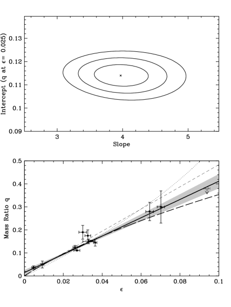
Figure 1: Calibration of the $q-\epsilon$ relation for superhumping CVs. Top panel: Constraints on the slope and intercept of the preferred linear calibration. The cross marks the best-fitting parameter combination. The ellipses correspond to 1$\sigma$, 2$\sigma$ and 3$\sigma$ contours on both parameters jointly. Bottom panel: Mass ratio vs period excess for the calibrating stars. The thick solid line is the best-fitting linear calibration, with the shaded area marking the statistical 1-$\sigma$ range. The thick long-dashed line shows P05’s calibration, the thin dotted line is Pearson’s (2006) calibration, and the thin short-dashed line is the calibration of Goodchild & Ogilvie (2006). The data point shown as a thin open symbol shows the upper limit on the mass ratio of BB Dor proposed by P05.

One final point worth noting is that the statistical errors on the fit parameters (and indeed the uncertainty regarding the functional form of the calibration itself) translate into systematic errors on the resulting masses and radii. The 1-$\sigma$ error band arising from the statistical uncertainties on our fit parameters is indicated by the dashed region in Figure 1. Formally, this is less than 10% even out to $q\simeq 0.4$, but the fit is very poorly constrained beyond $q\simeq 0.3$. The $\epsilon-q$ relation could thus change shape in this regime. The statistical error on a mass ratio obtained via Equation 7 can be estimated by folding the error on $\epsilon$ through the calibrating relation.

2.3 The Assumption of Constant Primary Mass

The next key step in the derivation of masses and radii from superhumpers is the assumption of a single primary mass for most systems in the sample. The worry here is not so much that the assumed mass might differ from the true mean WD mass for CVs. This would simply shift all ($\log{M_{2}}$, $\log{R_{2}}$) pairs along a line of slope 1/3, but would not alter the shape of the donor mass-radius relation. Instead, the main concern is that $M_{1}$ might exhibit systematic trends within the observed CV population, most importantly with orbital period. Such trends could affect the shape of the mass-radius relation.

In order to test whether this is a problem, we can check if there is any dependence of $M_{1}$ on $P_{orb}$ among CVs with reliable WD mass estimates (i.e. eclipsing systems). P05 actually tabulate all available $M_{1}$ estimates derived from eclipsing CVs. In the bottom panel of Figure 2, we plot these estimates as a function of $P_{orb}$ for all systems with $P_{orb}<6$ hrs. We exclude systems with longer periods, since they have evolved donors and thus follow a different evolution track (see Section 3.3 below).

Figure 2: Constraints on white dwarf mass evolution with orbital period. Top panel: Results of a linear fit to $M_{WD}$ vs $P_{orb}$ for eclipsing systems with well-determined white dwarf mass. The cross marks the best-fitting parameter combination. The ellipses correspond to 1$\sigma$, 2$\sigma$ and 3$\sigma$ contours on both parameters jointly. Bottom panel: $M_{WD}$ vs $P_{orb}$ for eclipsers. The thick solid line shows the optimally estimate mean white dwarf mass for all systems: $M_{WD}=0.75\pm 0.05M_{\odot}$ The thin dashed line shows the best linear fit to the data.

Figure 2 does not provide evidence for evolution of $M_{1}$ with $P_{orb}$. A full discussion of the statistical evidence for this assertion is given in Appendix B, along with a discussion of how this statement can be reconciled with earlier work that seemed to show such evolution. Here, we simply note that a linear fit to the data yields a slope consistent with zero. The best-fitting constant $M_{1}$ yields a mean WD mass of $<M_{1}>=0.75\pm 0.05M_{\odot}$ and requires an intrinsic scatter of $\sigma_{int}=0.16M_{\odot}$. Thus we confirm P05’s assertion that, in the absence of other information, $M_{1}$ can be estimated as $M_{1}=0.75M_{\odot}$ with about 20% uncertainty.

We finally note that the global intrinsic dispersion – $\sigma_{M_{1}}=0.16~{}M_{\odot}$, i.e. 21% – is the statistical error associated with taking $M_{1}=0.75M_{\odot}$ for any particular system. By contrast, the formal error on the mean WD mass ($0.05M_{\odot}$) translates into a systematic error on donor masses and radii (since a shift in the assumed $M_{1}$ affects all affected data points in the same way).

Having dealt with the $\epsilon-q$ calibration and the assumption of constant $M_{1}$, we are ready to calculate an updated set of $M_{2}$ and $R_{2}$ values (with statistical errors) for all superhumpers. We list these in Table 1. Our estimates are not identical to those derived by P05, since we have used a different $\epsilon-q$ calibration and have explicitly accounted for the intrinsic dispersion in $M_{1}$ when estimating the statistical errors. However, as expected, the overall pattern presented by the data is much the same. The main change in the data values is a slight shift towards higher masses, which arises because our $q$-estimates are generally a little higher than P05’s for fixed $\epsilon$ (see Figure 1).

2.4 External Constraints: The Location of the Period Gap and the Minimum Period

In principle, we could now simply fit the $M_{2}-R_{2}$ pairs in Table 1 (supplemented with data for eclipsing systems). However, there are actually additional empirical constraints that can (and should) be imposed on the mass-radius relation. These constraint come from the observed locations of the period gap and of the period minimum.

Let us first consider the period gap. The bottom panel in Figure 3 shows the $M_{2}-R_{2}$ estimates from Table 1, along with similar data for eclipsing systems, taken from Table 8 in P05. There is a clear discontinuity in donor radii at $M_{2}\simeq 0.2M_{\odot}$, with donors in long-period systems being larger than those in short-period systems. As discussed in more detail by P05, the transition is quite sharp and broadly consistent with the standard CV evolution scenario. Briefly, we should expect systems just above and below the period gap to have identical donor masses, since CVs evolve through the period gap as detached binaries, with no significant mass loss from the secondary. However, their radii must differ, since both short- and long-period donors must still obey the period-density relation for Roche-lobe- filling stars (Equation 3). More specifically, if we denote the upper and lower edges of the period gap as $P_{gap,\pm}$, the ratio of donor radii at the gap edges must satisfy

$$\frac{R_{2,+}}{R_{2,-}}=\left(\frac{P_{gap,+}}{P_{gap,-}}\right)^{2/3}.$$ (8)

Physically, donors above the gap are larger since they lose mass at a much higher rate than those below and are therefore forced more out of thermal equilibrium.

If we accept the premise that CV donors evolve through the period gap as detached systems, the data in Figure 3 suggests that the critical donor mass at which mass transfer stops (and then restarts) is $M_{conv}=0.20\pm 0.02M_{\odot}$, where the estimated error is purely statistical. In other words, $M_{conv}$ is the donor mass at both edges of the period gap. Given empirical estimates for the location of these edges, we can therefore use the period-density relation to determine $R_{2,conv}$, i.e. the radii of donors at the gap edges. Thus the locations of the gap edges ($P_{gap,\pm}$) fix the $M_{2}-R_{2}$ relations for long- and short-period systems at $M_{conv}$ and $P_{gap,\pm}$.

Figure 4 shows the orbital period distribution of CVs drawn from the Ritter & Kolb (2003) catalog (Edition 7.6) in both differential and cumulative form. The period gap is obvious in these distributions. We have carried out repeated measurements of the gap edges from this data with a variety of binning schemes. Based on these measurements, we estimate $P_{gap,-}=2.15\pm 0.03$ hrs and $P_{gap,+}=3.18\pm 0.04$ hrs. It is worth noting that the number of systems inside the gap increases towards longer periods. This may be due to low-metallicity systems, which are expected to invade the gap from above (Webbink & Wickramasinghe 2002).

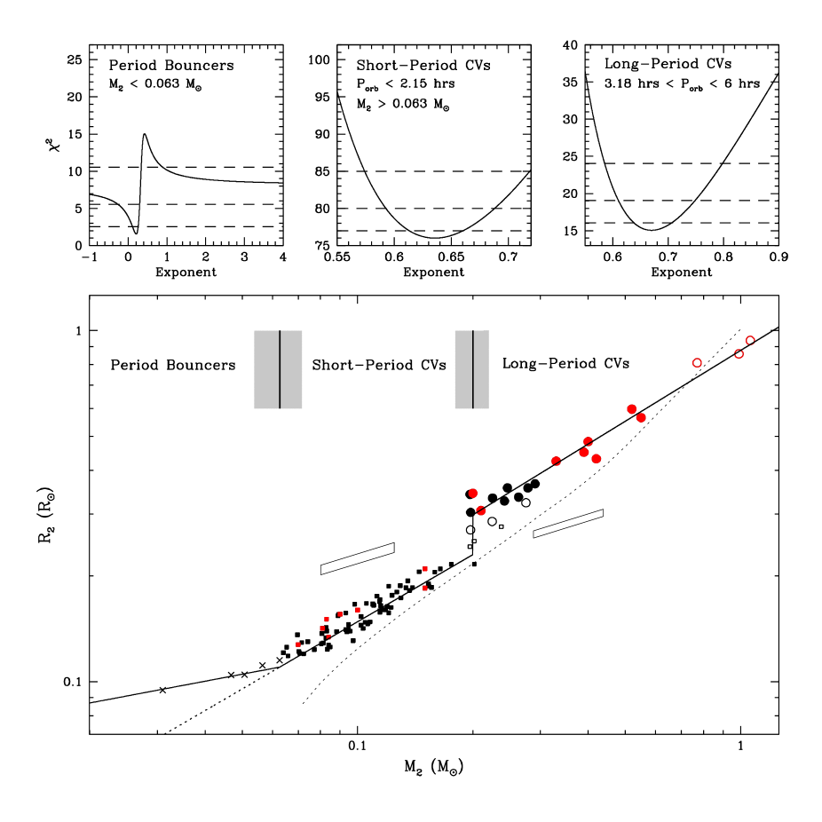
Figure 3: The mass-radius relation of CV donor stars. Bottom panel: Points shown are empirical mass and radius estimates for CV donors. Superhumpers are shown in black, eclipsers in red. Filled squares correspond to short-period CVs, filled circles to long-period systems, and crosses to likely period bouncers. The parallelograms illustrate the typical error on a single short-period or long-period CV. Open symbols were ignored in fits to the data since they correspond to systems in the period gap or long-period (probably evolved) systems. The solid lines show the optimal fit to the data in the period bouncer, short-period and long-period regions. The dotted line is the mass-radius relation for main sequence stars taken from the 5 Gyr BCAH98 isochrone. Top panels: Constraints on the power law exponents of the $M_{2}-R_{2}$ relations in the three period/mass regimes. For each regime, we plot $\chi^{2}$ vs exponent and indicate the $\chi^{2}$ corresponding to 1-$\sigma$, 2-$\sigma$ and 3-$\sigma$ around the minimum with horizontal dashed lines. The strange shape of the $\chi^{2}$ curve for the period bouncers near the exponent $\frac{1}{3}$ is real. It arises because the intrinsic power law relationship between $M_{2}$ and $R_{2}$ estimates has the same exponent.

Table 1: Donor masses and radii as estimated from superhump periods. Orbital periods are in hours; masses and radii are in solar units. Note that mass and radius estimates are not independent, but correlated via Equation 6.

System	$P_{orb}$	$M_{2}$	$\sigma_{M_{2}}$	$R_{2}$	$\sigma_{R_{2}}$		System	$P_{orb}$	$M_{2}$	$\sigma_{M_{2}}$	$R_{2}$	$\sigma_{R_{2}}$
DI UMa	1.3094	0.051	0.011	0.105	0.008		CY UMa	1.6697	0.119	0.026	0.164	0.012
V844 Her	1.3114	0.083	0.018	0.124	0.009		FO And	1.7186	0.115	0.027	0.165	0.013
LL And	1.3212	0.097	0.023	0.131	0.010		OU Vir	1.7450	0.130	0.029	0.173	0.013
SDSS 0137-09	1.3289	0.085	0.019	0.125	0.009		VZ Pyx	1.7597	0.110	0.024	0.165	0.012
ASAS 0025+12	1.3452	0.072	0.017	0.120	0.009		CC Cnc	1.7645	0.156	0.034	0.186	0.014
AL Com	1.3601	0.047	0.010	0.104	0.008		HT Cas	1.7676	0.089	0.009	0.154	0.005
WZ Sge	1.3606	0.056	0.009	0.111	0.006		IY UMa	1.7738	0.093	0.006	0.157	0.003
RX 1839+26	1.3606	0.063	0.015	0.115	0.009		VW Hyi	1.7825	0.110	0.024	0.166	0.012
PU CMa	1.3606	0.077	0.018	0.123	0.009		Z Cha	1.7880	0.089	0.003	0.155	0.001
SW UMa	1.3634	0.084	0.020	0.127	0.010		QW Ser	1.7887	0.110	0.026	0.167	0.013
HV Vir	1.3697	0.071	0.015	0.120	0.009		WX Hyi	1.7954	0.114	0.025	0.169	0.012
MM Hya	1.3822	0.066	0.014	0.118	0.009		BK Lyn	1.7995	0.154	0.033	0.187	0.013
WX Cet	1.3990	0.070	0.016	0.122	0.009		RZ Leo	1.8250	0.114	0.026	0.171	0.013
KV Dra	1.4102	0.080	0.018	0.128	0.010		AW Gem	1.8290	0.137	0.030	0.182	0.013
T Leo	1.4117	0.081	0.018	0.129	0.009		SU UMa	1.8324	0.105	0.023	0.167	0.012
EG Cnc	1.4393	0.031	0.007	0.095	0.007		SDSS 1730+62	1.8372	0.123	0.027	0.176	0.013
V1040 Cen	1.4467	0.103	0.023	0.142	0.011		HS Vir	1.8456	0.153	0.033	0.190	0.014
RX Vol	1.4472	0.064	0.015	0.121	0.009		V503 Cyg	1.8648	0.139	0.031	0.185	0.014
AQ Eri	1.4626	0.096	0.021	0.139	0.010		V359 Cen	1.8696	0.127	0.030	0.180	0.014
XZ Eri	1.4678	0.094	0.005	0.139	0.003		CU Vel	1.8840	0.098	0.024	0.166	0.013
CP Pup	1.4748	0.083	0.015	0.133	0.008		NSV 9923	1.8984	0.134	0.030	0.185	0.014
V1159 Ori	1.4923	0.106	0.023	0.146	0.010		BR Lup	1.9080	0.112	0.027	0.175	0.014
V2051 Oph	1.4983	0.095	0.022	0.141	0.011		V1974 Cyg	1.9502	0.202	0.033	0.216	0.012
V436 Cen	1.5000	0.074	0.018	0.130	0.011		TU Crt	1.9702	0.129	0.028	0.188	0.014
BC UMa	1.5026	0.102	0.022	0.145	0.010		TY PsA	2.0194	0.135	0.030	0.194	0.014
HO Del	1.5038	0.093	0.022	0.141	0.011		KK Tel	2.0287	0.121	0.027	0.187	0.014
EK TrA	1.5091	0.107	0.024	0.147	0.011		V452 Cas	2.0304	0.159	0.035	0.205	0.015
TV Crv	1.5096	0.108	0.025	0.148	0.011		DV UMa	2.0604	0.165	0.013	0.209	0.006
VY Aqr	1.5142	0.072	0.016	0.129	0.010		YZ Cnc	2.0832	0.176	0.038	0.216	0.016
OY Car	1.5149	0.065	0.004	0.125	0.003		GX Cas	2.1365	0.145	0.032	0.206	0.015
RX 1131+43	1.5194	0.088	0.019	0.139	0.010		NY Ser	2.3460	0.197	0.043	0.242	0.018
ER UMa	1.5278	0.105	0.023	0.148	0.011		V348 Pup	2.4442	0.202	0.045	0.251	0.019
DM Lyr	1.5710	0.095	0.022	0.145	0.011		V795 Her	2.5982	0.237	0.051	0.276	0.020
UV Per	1.5574	0.081	0.019	0.137	0.010		V592 Cas	2.7614	0.197	0.042	0.270	0.019
AK Cnc	1.5624	0.121	0.028	0.157	0.012		TU Men	2.8128	0.225	0.049	0.286	0.021
AO Oct	1.5737	0.083	0.021	0.139	0.012		AH Men	3.0530	0.275	0.059	0.323	0.023
SX LMi	1.6121	0.114	0.026	0.158	0.012		DW UMa	3.2786	0.197	0.010	0.303	0.005
SS UMi	1.6267	0.118	0.026	0.160	0.012		TT Ari	3.3012	0.263	0.056	0.335	0.024
KS UMa	1.6310	0.083	0.020	0.143	0.011		V603 Aql	3.3144	0.242	0.044	0.327	0.020
V1208 Tau	1.6344	0.122	0.027	0.163	0.012		PX And	3.5124	0.278	0.060	0.356	0.025
RZ Sge	1.6387	0.102	0.023	0.153	0.012		V533 Her	3.5352	0.225	0.048	0.333	0.024
TY Psc	1.6399	0.114	0.025	0.159	0.012		BB Dor	3.5808	0.291	0.062	0.366	0.026
IR Gem	1.6416	0.116	0.032	0.160	0.015		BH Lyn	3.7380	0.246	0.053	0.356	0.026
V699 Oph	1.6536	0.070	0.017	0.136	0.011		UU Aqr	3.9259	0.197	0.041	0.342	0.024

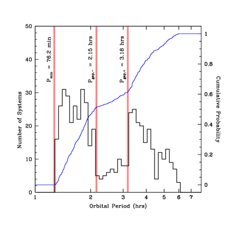
Figure 4: Differential and cumulative orbital period distribution of CVs, based on data taken from Edition 7.6 of the Ritter & Kolb (2003) catalog. Our adopted values for the minimum period and the period gap edges are shown as vertical lines. The shaded regions around them indicate our estimate of the errors on these values.

We can similarly demand that our mass-radius relationship should reproduce the observed minimum period, $P_{min}$, of the CV population. Based again on the data in Figure 4, we estimate this to be $P_{min}=76.2\pm 1.0$ min. We can implement this constraint by truncating the $M_{2}-R_{2}$ relation for short-period CVs at $M_{bounce}$, the donor mass where it reaches $P_{min}$. If there are data points with lower masses, they need to be fit separately, subject to the constraint that the fit should meet the mass-radius relation for short-period CVs at $M_{bounce}$. Moreover, if $P_{min}$ is supposed to be a minimum period, then the fit to systems with $M_{2}<M_{bounce}$ should yield an $M_{2}-R_{2}$ relation that corresponds to increasing orbital period with decreasing $M_{2}$. We will find below that that is indeed the case.

2.5 The Optimal $M_{2}$-$R_{2}$ Relation for CV Donors

Given our set of mass-radius pairs and the added external constraints, how can we obtain an optimal analytical description of the overall $M_{2}-R_{2}$ relation? This question is not as trivial as it may seem, for two reasons. First, the external constraints (i.e. the measured values of $P_{min}$, $P_{gap,\pm}$ and $M_{conv}$) need to be imposed self-consistently on fits to the $M_{2}-R_{2}$ pairs. Second, the mass and radius estimates for any given superhumper (along with their errors) are completely correlated. This was already pointed out by P05 and is easy to see from Equation 6, which shows that $R_{2}\propto M_{2}^{1/3}$. The masses and radii of eclipsers are similarly correlated, since only $q$ and $M_{1}$ are generally estimated directly from the light curve, with $M_{2}$ and $R_{2}$ being obtained indirectly in much the same way as for superhumpers. This correlation should be taken into account when fitting the data.

In Appendix C, we show how the standard $\chi^{2}$-statistic can be modified so as to explicitly account for correlated data points, external constraints and intrinsic dispersion. When carrying out our $\chi^{2}$ fits, we explicitly distinguish between three groups of CVs, each of which is fit independently with a power-law $M_{2}-R_{2}$ relation: (i) non-evolved long-period CVs ($3.18$ hrs $<P_{orb}<6$ hrs); (ii) “normal” short-period CVs ($P_{orb}<2.15~{}hrs$ and $M_{2}>M_{bounce}$; (iii) period bouncers ($M_{2}<M_{bounce}$). The value of $M_{bounce}$ is obtained from the fit to short-period CV, as described in Section 2.4. In principle, this could be an iterative procedure, since the value of $M_{bounce}$ determines which points are included in the fit. In practice, the fit to the short-period systems is quite insensitive to the exact value, since the vast majority of points lie well above any plausible estimate for $M_{bounce}$. For the optimal fit described below, we find $M_{bounce}=0.0626M_{\odot}$.

Remarkably, we find that the intrinsic radius scatter required by the $\chi^{2}$ fits to the short- and long-period systems is only about 2%-3%. For comparison, the typical statistical error is about 7%-8%. This implies that the intrinsic dispersion is probably rather poorly constrained by the data, but also that it cannot be more than a few percent. Thus there really is a unique evolution track that is followed by almost all CVs. When other tracers are used to study CV evolution (e.g. luminosity or period changes), the existence of this track is often masked by variability on time scales shorter than the binary evolution time scale (e.g. Büning & Ritter 2004). However, donor radii are hardly affected by these short-time-scale effects and thus faithfully trace the long-term evolution of $\dot{M}_{2}$

Our final mass-radius relation for all three types of CV donors is given by:

$$\tiny\frac{R_{2}}{R_{\odot}}=\left\{\begin{array}[]{ll}(0.110\pm 0.005)\times\left(\frac{M_{2}}{M_{bounce}}\right)^{0.21^{+0.05}_{-0.10}}&{\rm Period~{}Bouncers}\\ &\\ (0.230\pm 0.008)\times\left(\frac{M_{2}}{M_{conv}}\right)^{0.64\pm 0.02}&{\rm Short-Period~{}CVs}\\ &\\ (0.299\pm 0.010)\times\left(\frac{M_{2}}{M_{conv}}\right)^{0.67\pm 0.04}&{\rm Long-Period~{}CVs}\\ \end{array}\right.$$ (9)

where the three regimes are formally defined as (i) period bouncers: $M_{2}<M_{bounce}$; (ii) short-period CVs: $M_{bounce}<M_{2}<M_{conv}$ and $P_{orb}<P_{gap,-}$; (iii) long-period CVs: $M_{conv}<M_{2}<M_{evol}$ and $P_{gap,+}<P_{orb}<P_{evol}$. For reference, let us also summarize the various quantities that have been assumed

$$\begin{array}[]{lll}M_{bounce}&=&0.063\pm 0.009~{}M_{\odot}\\ M_{conv}&=&0.20\pm 0.02~{}M_{\odot}\\ M_{evol}&\simeq&0.6-0.7~{}M_{\odot}\\ P_{min}&=&76.2\pm 1.0~{}{\rm min}\\ P_{gap,-}&=&2.15\pm 0.03~{}{\rm hr}\\ P_{gap,+}&=&3.18\pm 0.04~{}{\rm hr}\\ P_{evol}&\simeq&5-6~{}{\rm hr}.\end{array}$$ (10)

We note in passing that the best-fitting mass-radius relation in the short-period regime is slightly steeper than might be suggested by visual inspection of the data in Figure 3. This is because $M_{2}$ and $R_{2}$ are correlated. More specifically, the appearance of the power law index $b$ in Equation 23 acts to push the fit away from indeces $b\simeq\frac{1}{3}$ and thus in this case to larger values. This can be verified by artificially increasing the assumed intrinsic dispersion, since this forces the fit towards a standard least-squares solution. As expected, the power law index then tends to a slightly shallower value of 0.60 in the short-period regime, and the donor mass at period minimum becomes $M_{bounce}=0.053M_{\odot}$.

P05 did not derive a fit to the period bouncers, due to the sparseness of the donor data in the sub-stellar regime. We completely agree with P05 that the fit is very poorly constrained for this group: only 5 data points fall into this class in our sample, and only one of these is clearly inconsistent with the $M_{2}-R_{2}$ relation for “ordinary” short-period systems. The $M_{2}-R_{2}$ relation in this regime is thus strongly affected by our estimate for $P_{min}$ and by the parameters inferred for short-period systems. These constraints ultimately decide which points are included in the period bouncer class and also uniquely fix $R_{2}$ at $M_{bounce}$. We have nevertheless provided the best-fit parameters for this group, partly because we have no reason to distrust these constraints, and partly because we want our semi-empirical donor sequence to extend into the sub-stellar (period bounce) regime; we would therefore rather have an uncertain mass-radius relation than none.

We also derive some confidence in our fit to the period bouncers from the fact that the best-fit mass-radius exponent in this regime turns out to be less than 1/3 (at somewhat better than 2-$\sigma$). This is a critical value, because the effective mass-radius index of the donor determines the sign of the period derivative of a CV. This can be seen explicitly by combining Paczyniski’s (1971) approximation for the radius of Roche-lobe-filling secondaries

$$\frac{R_{2}}{a}=0.462\left(\frac{q}{1+q}\right)^{1/3}$$ (11)

(which is valid for $q\raisebox{-2.58334pt}{$\;\stackrel{{\scriptstyle\raisebox{-0.60275pt}{$\textstyle<$}}}{{\sim}}\;$}0.8$) with Kepler’s third law to obtain

$$\frac{\dot{P_{orb}}}{P_{orb}}=\frac{3\xi-1}{2}\frac{\dot{M}_{2}}{M_{2}}.$$ (12)

Here, $\dot{M}_{2}<0$ is the mass transfer rate from the donor, and $\xi$ is the effective mass-radius index of the donor along its evolutionary track. If the mass-radius relation along the track can be described as a power law, $\xi$ is simply the power-law exponent. Equation 12 shows that the orbital period decreases for $\xi>1/3$, but increases for $\xi<1/3$. With $\xi=0.21^{+0.05}_{-0.10}$ for our period bouncers, these systems appear to be evolving back towards larger periods – as they should, since $P_{min}$ is supposed to be a minimum period along our donor track.

3 The Late Spectral Types of CV Donors

We now turn our attention to the spectral types of CV donors, and specifically to the $SpT$-$P_{orb}$ relationship. Ultimately, our goal will be to test if donor models based on the $M_{2}-R_{2}$ relations we have just derived are capable of reproducing the empirical $SpT$-$P_{orb}$ relation. However, our immediate task in this section is mainly the construction of an updated compilation of spectroscopic $SpT$ determinations for CV donors. We will also carry out a direct comparison between this sample and a sample of isolated MS stars. This will allow us to establish the extent of any $SpT$ discrepancy between CV donors and MS stars as a function of orbital period.

3.1 An Updated Sample of Spectral Types for CV Secondaries

B98 presented a compilation of 54 spectroscopically established donor $SpT$s for CVs with $P_{orb}<12$ hrs. Since then, many improved and new $SpT$ estimates have become available. We therefore felt it was worth repeating their analysis in order to increase the reliability and size of the donor $SpT$ sample. Briefly, we extracted a list of all $SpT$ estimates for CVs with $P_{orb}<12$ hrs from the latest version of the Ritter & Kolb (2003) catalog (Edition 7.6). We inspected all of the original references for these $SpT$s and rejected all purely photometric $SpT$ determinations, and also a few spectroscopic estimates that we considered to be less compelling. In some cases, we also carried out additional literature searches and adjusted the $SpT$s and their errors to provide best-bet estimates based on all of the available evidence. Where no new information was available, we generally retained B98’s $SpT$ estimates, with two noteworthy exceptions: we were unable to find any reliable spectroscopic $SpT$ determinations for OY Car and QZ Aur in the literature. We therefore removed these objects from our database. Our final compilation is provided in Table 2 and contains 91 $SpT$s.

Table 2: Spectral types of CV donors. This table is an update of the compilation provided by B98. It is based, in the first instance, on the $SpT$ estimates contained in the latest version (Edition 7.6) of the Ritter & Kolb (2003) catalog. However, all original source material was inspected, and only spectroscopically determined $SpT$s that were deemed reliable were accepted. In some cases (e.g. where more than one $SpT$ estimate was available in the literature), the adopted $SpT$s and/or errors were adjusted to provide best-bet estimates based on all of the available evidence.

System	$P_{orb}$ (hrs)	Spectral Type		System	$P_{orb}$ (hrs)	Spectral Type
RX J1951	11.808	M0 $\pm$ 0.5		GY Cnc	4.211	M3 $\pm$ 1
UY Pup	11.502	K4 $\pm$ 2		SDS J2048	4.200	M3 $\pm$ 1
V442 Cen	11.040	G6 $\pm$ 2		V1043 Cen	4.190	M2.5 $\pm$ 0.5
DX And	10.572	K0 $\pm$ 1		SDSS J0924	4.056	M3.5 $\pm$ 1
AE Aqr	9.880	K4 $\pm$ 1		DO Dra	3.969	M4.25$\pm$ 0.7
1RXS J1548	9.864	K2 $\pm$ 2		UU Aql	3.925	M4 $\pm$ 1
AT Ara	9.012	K2 $\pm$ 0.5		CN Ori	3.917	M4 $\pm$ 1
RU Peg	8.990	K2.5 $\pm$ 0.5		KT Per	3.905	M3.3 $\pm$ 1
GY Hya	8.336	K4.5 $\pm$ 0.5		CY Lyr	3.818	M3.25$\pm$ 1.25
CH UMa	8.236	K6.5 $\pm$ 1.5		VY For	3.806	M4.5 $\pm$ 1
MU Cen	8.208	K4 $\pm$ 1		IP Peg	3.797	M4 $\pm$ 0.5
BT Mon	8.012	G8 $\pm$ 2		QQ Vul	3.708	M4 $\pm$ 0.5
V1309 Ori	7.983	M0.5 $\pm$ 0.5		WY Sge	3.687	M4 $\pm$ 1
V392 Hya	7.799	K5.5 $\pm$ 0.5		RX J0944	3.581	M2 $\pm$ 1
AF Cam	7.776	K5.5 $\pm$ 2		MN Hya	3.390	M3.5 $\pm$ 0.5
V363 Aur	7.710	G7 $\pm$ 2		V1432 Aql	3.366	M4 $\pm$ 0.5
RY Ser	7.222	K5 $\pm$ 1		TT Ari	3.196	M3.5 $\pm$ 0.5
AC Cnc	7.211	K2 $\pm$ 1		MV Lyr	3.190	M5 $\pm$ 0.5
EM Cyg	6.982	K3 $\pm$ 1		SDSS J0837	3.180	M5 $\pm$ 1
Z Cam	6.956	K7 $\pm$ 2		AM Her	3.094	M4.25$\pm$ 0.5
SDSS J0813	6.936	K5.5 $\pm$ 1		WX LMi	2.782	M4.5 $\pm$ 2
V426 Oph	6.848	K5 $\pm$ 1		RX J1554	2.531	M4 $\pm$ 1
SS Cyg	6.603	K4.5 $\pm$ 0.5		SDSS J1702	2.402	M1.5 $\pm$ 1.1
CW 1045	6.511	K6.5 $\pm$ 1.5		QS Tel	2.332	M4.5 $\pm$ 0.5
CM Phe	6.454	M3.5 $\pm$ 1.5		UW Pic	2.224	M4.5 $\pm$ 1
TT Crt	6.440	K5 $\pm$ 0.75		UZ For	2.109	M4.5 $\pm$ 0.5
BV Pup	6.353	K3 $\pm$ 2		HU Aqr	2.084	M4.25$\pm$ 0.7
AH Her	6.195	K7 $\pm$ 1		DV UMa	2.063	M4.5 $\pm$ 0.5
XY Ari	6.065	M0 $\pm$ 0.5		QZ Ser	1.996	K4 $\pm$ 2
LL Lyr	5.978	M2.5 $\pm$ 1.5		AR UMa	1.932	M5.5 $\pm$ 0.5
AH Eri	5.738	M4 $\pm$ 1		ST LMi	1.898	M5.5 $\pm$ 1.5
V347 Pup	5.566	M0.5 $\pm$ 0.5		MR Ser	1.891	M6 $\pm$ 1
RW Tri	5.565	M0 $\pm$ 1		CU Vel	1.884	M5 $\pm$ 1
EZ Del	5.362	M1.5 $\pm$ 0.5		V2301 Oph	1.883	M5.5 $\pm$ 1
CZ Ori	5.254	M2.5 $\pm$ 1.5		RZ Leo	1.836	M5 $\pm$ 1
AR Cnc	5.150	M5 $\pm$ 1		Z Cha	1.788	M5.5 $\pm$ 0.5
EX Dra	5.038	M1.5 $\pm$ 0.5		HT Cas	1.768	M5.4 $\pm$ 0.3
RX And	5.037	K4.75$\pm$ 2		V834 Cen	1.692	M6.5 $\pm$ 1.5
AT Cnc	4.826	K7.5 $\pm$ 1		VV Pup	1.674	M6.5 $\pm$ 1
DQ Her	4.647	M3 $\pm$ 0.5		EX Hya	1.638	M4 $\pm$ 1
AI Tri	4.602	M2.5 $\pm$ 1		HS Cam	1.637	M5 $\pm$ 2
Leo 7	4.483	M3 $\pm$ 1		BZ UMa	1.632	M5.5 $\pm$ 0.5
SDSS J1553	4.391	M4.5 $\pm$ 1		VY Aqr	1.514	M9.5 $\pm$ 1
SS Aur	4.387	M3 $\pm$ 1		BC UMa	1.512	M6.5 $\pm$ 0.5
TW Vir	4.384	M5.5 $\pm$ 0.5		EI Psc	1.070	K5 $\pm$ 1
U Gem	4.246	M4.25$\pm$ 0.5

3.2 A Benchmark Main Sequence Sample

In order to assess the departure of CV donors from thermal equilibrium, we need a comparison sample of $SpT$s for MS stars. We use the $[M/H]\simeq 0$ sample compiled by Beuermann et al. (1999; hereafter B99) for this purpose. This is based on source data from Leggett et al. (1996; B99 Table 2) and Henry & McCarthy (1993; B99 Table 3). Three unresolved binaries were removed from the sample, and one missing spectral sub-type (GD165B: $SpT$=L4) was added from Leggett et al. (2001). In order to better cover the late-M and L dwarf regime, we also added a few late-type, solar metallicity objects from Leggett et al. (2001). These again included some unresolved binaries, but since data is so sparse in this regime we did not reject these objects outright. Instead, we use these binaries only for calibrating the $SpT-(I-K)$ relation (see below), where blending of objects with similar $SpT$ should not introduce any serious errors. Finally, we also added the Sun ($SpT$=G2) and Gl34A ($SpT$=G3) as calibrators, in order to extend the MS sample into the G-dwarf regime. $SpT$s and absolute magnitudes for these two objects were taken from B98. Overall, however, we prefer the B99 MS sample to that used by B98 since probable low-metallicity objects have been removed from the former.

In addition to providing an empirical comparison sample for CV donors, the MS sample is also useful for testing and calibrating the stellar models we will use in constructing our semi-empirical donor sequence. Of particular importance in this context is the ability of the models to reproduce the observed I-K colours along the MS, since we will follow B98 in using this colour to estimate $SpT$s for the models.

So how well do up-to-date stellar models reproduce the I-K colours of MS stars? In Figure 5 we show the $M_{K}$ vs (I-K) CMD for our MS sample, along with two sets of MS models. The first is the 5 Gyr isochrone taken from Baraffe et al. (1998; hereafter BCAH98), with colours calculated from the NextGen model atmospheres (Hauschildt, Allard & Baron 1999). The second, which we call AMES-MT, is an updated version of the BCAH98 models and has been suggested to provide a somewhat better match to observed optical colours (Allard, Hauschildt & Schwenke 2000). The main difference between the BCAH98 and AMES-MT models is the inclusion of an updated TiO line list in the latter.

Somewhat surprisingly, Figure 5 shows that the older BCAH98 isochrone does a much better job of fitting the empirical $M_{K}$ vs (I-K) CMD. We can only conclude that the AMES-MT models have achieved their improvement in the optical region at the expense of the (near-)infrared. Given the crucial importance of the latter region for our purposes, we use the BCAH98/NextGen models throughout this paper.

We finally revisit the $SpT$-$(I-K)$ relation defined by our MS sample. This is shown in Figure 6. Since our sample is substantially the same as that used by B98, their third order polynomial fit remains a good description of the data over most of its range. However, since our new sample now includes a mid-L dwarf (whereas B98’s calibrating sample did not extend beyond M8), it makes sense to redetermine the polynomial coefficients to ensure that the fit also describes this very late-type regime. Figure 6 shows our new calibration, which is given by

$$X=56.92-35.21(I-K)+9.810(I-K)^{2}-0.9450(I-K)^{3},$$ (13)

where $SpT=L(10-X)$ for $X\leq 10$, $SpT=M(20-X)$ for $10<X\leq 20$, $SpT=K(28-X)$ for $20<X\leq 28$, and $SpT=G(38-X)$ for $28<X\leq 38$. Note that in order to make room for L-dwarfs, we have shifted the $SpT$-$X$ relation (and hence the constant term of the polynomial fit) relative to that used by B98. As expected, our fit parameters differ only slightly from those derived by B98, but the new fit does indeed provide an improved match to the latest calibrators. The RMS scatter around the polynomial fit is less than 0.5 sub-types for L0 $<$ $SpT$s $<$ K5 but increases to 1-2 sub-types outside this range.

Figure 5: The I-K colour-magnitude diagram for the solar-metallicity main sequence sample. The solid line shows the 5 Gyr BCAH98 isochrone, which is based on the NextGen atmosphere models of Hauschildt, Allard & Baron (1999). The dashed line corresponds to a 5 Gyr isochrone based on a later version of these models (AMES-MT), which makes use of an updated TiO line list (Allard, Hauschildt & Schwenke 2000). Note that the BCAH98 models actually provide a much better match to the data.

3.3 CV Donors vs Main Sequence Stars

In Figure 7 we compare the $SpT$s of CV donors and MS stars. We follow B98 in presenting this comparison in the $SpT$-$P_{orb}$ plane. For this purpose, each star in the MS sample is assigned an orbital period on the basis of its mass and radius via the period-density relation for Roche-lobe-filling stars; thus the assigned $P_{orb}$ is the period of a hypothetical semi-detached system in which the MS star is the mass donor.

This calculation requires masses and radii for all of the stars in our MS sample. We estimate masses from the theoretical K-band mass-luminosity relation – $M(M_{K})$ – predicted by the BCAH98 models. In principle, it would be preferable to use an empirical calibration for this purpose, in order to avoid artificially forcing the data points close to the models in the $P_{orb}-SpT$ plane. However, the best empirical $M(M_{K})$ relation (Delfosse et al. 2000) is only calibrated over the range $4.5<M_{K}<9.5$, which excludes the earliest and latest stars in our sample. Moreover, Figure 3 in Delfosse et al. (2000) shows that the theoretical and empirical relations agree very closely in the well-calibrated regime, but there are hints that beyond this range, their 5th-order polynomial fit becomes less reliable than the theoretical models. In any case, we have checked that adopting the Delfosse et al. $M(M_{K})$ relation (even beyond its region of validity) would not change any of our conclusions.

Several radius estimates for the stars in our MS sample are available from B99 and Leggett et al. (2001). The bulk of our sample comes from B99, who provide three radius estimates for each star. These are based on (i) the $S_{K}(V-K)$ relation for MS stars, where $S_{K}$ is the K-band surface brightness (see also Section 4.3); (ii) the $S_{K}(I-K)$ relation; (iii) the $R_{2}(M_{K})$ relation. B99 show that all of these estimates are probably good to better than 5%. We adopt the average of these estimates and use their range as a measure of the associated error on the radius (and hence on the assigned orbital period).

Figure 7 also shows the $SpT$-$P_{orb}$ relation predicted by the BCAH98 5 Gyr isochrone. For this purpose, periods were assigned to the models in the same way as for the MS stars (i.e. based on the model masses and radii), and $SpT$s were estimated from Equation 13.

Figure 6: The spectral type vs (I-K) relation for the solar metallicity main sequence sample. The line shows the third order polynomial fit given by Equation 13.

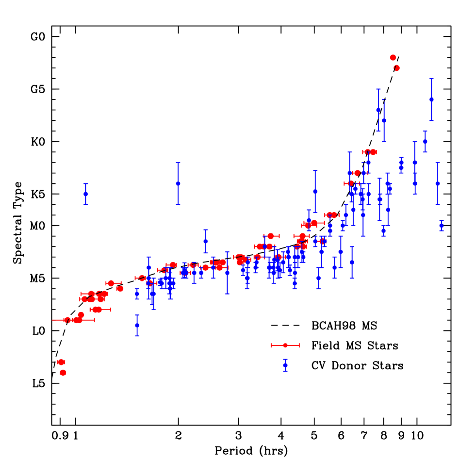
Figure 7: The empirical spectral type - orbital period relation for CVs and main sequence stars. Blue points are CV donors from Table 2, red points are MS stars. The dashed line is the relation predicted by the 5 Gyr BCAH98 isochrone, with the $SpT$(I-K) calibration given by Equation 13.

Several important results emerge immediately. First, the $SpT$-$P_{orb}$ relation of MS stars is fairly well described by the BCAH98 model sequence. Second, the $SpT$s of CV donors are systematically later than those of isolated MS stars. Importantly, this is the case across the entire $P_{orb}$ range, not just for long-period systems with $P_{orb}\raisebox{-2.58334pt}{$\;\stackrel{{\scriptstyle\raisebox{-0.60275pt}{$\textstyle>$}}}{{\sim}}\;$}3$ hrs, as suggested by B98. (With hindsight, we think that a discrepancy between the $SpT$s of CV donors and MS models at short periods was already somewhat noticeable from Figs. 4 and 5 of B98.) Third, apart from a few outliers, the CV donors with $P_{orb}\raisebox{-2.58334pt}{$\;\stackrel{{\scriptstyle\raisebox{-0.60275pt}{$\textstyle<$}}}{{\sim}}\;$}5-6$ hrs define a remarkably consistent $SpT$-$P_{orb}$ sequence. This is again evidence that most CVs do indeed follow a standard evolutionary track with relatively little scatter. Fourth, at longer periods, $P_{orb}\raisebox{-2.58334pt}{$\;\stackrel{{\scriptstyle\raisebox{-0.60275pt}{$\textstyle>$}}}{{\sim}}\;$}5-6$ hrs, the $SpT$ scatter increases markedly, although the donors remain cooler than MS stars at the same period.

B98 already provided a promising explanation for the appearance of the $SpT$-$P_{orb}$ diagram at $P_{orb}\raisebox{-2.58334pt}{$\;\stackrel{{\scriptstyle\raisebox{-0.60275pt}{$\textstyle>$}}}{{\sim}}\;$}5-6$ hrs. More specifically, they showed that donors that are already somewhat nuclear-evolved at the start of mass transfer move through just the region of the $SpT$-$P_{orb}$ diagram that is occupied by observed systems. The increased scatter in $SpT$s at the longest periods could then be understood as reflecting the range of central Hydrogen abundances in these donors at the start of mass transfer. The viability of this idea was confirmed by Baraffe & Kolb (2000) and Podsiadlowski, Han & Rappaport (2003). In the latter work, the authors also found that the dominance of evolved systems above $P_{orb}\simeq 5$ hrs (and the dominance of unevolved systems at shorter periods) is actually expected, even if evolved systems comprise only a small percentage of the total CV population. For the record, the semi-empirical donor sequence constructed below is intended to describe the unique evolution track followed by unevolved donors, and we therefore limit it to $P_{orb}\raisebox{-2.58334pt}{$\;\stackrel{{\scriptstyle\raisebox{-0.60275pt}{$\textstyle<$}}}{{\sim}}\;$}6$ hrs.

We finally comment briefly on the three most striking outliers in Figure 7, namely the three systems that lie significantly above the standard MS track with $P_{orb}<3$ hrs. In order of decreasing period, these systems (and their spectral type references) are SDSS J1702+3229 (Szkody et al. 2004), QZ Ser (Thorstensen et al. 2002a) and EI Psc (Mennickent et al. 2004; see also Thorstensen et al. 2002b). This part of the $SpT$-$P_{orb}$ diagram should only be populated by low-metallicity systems (B98) or again by systems in which the donor was already significantly evolved at the onset of mass-transfer. At least for QZ Ser and EI Psc, the latter is the preferred explanation and can also account for the fact that the orbital period of EI Psc ($P_{orb}=64$ min) is well below the minimum period for “normal” CVs (Thorstensen et al. 2002ab). SDSS J1702+3229 is located within the period gap ($P_{orb}=2.4$ hrs), and the $SpT$ estimate for it is based on the TiO-band strength measured by Szkody et al. (2004). This system is only about 2 $\sigma$ above the “standard” CV donor sequence, so additional observations will be needed to confirm if this system is genuinely abnormal.

4 A Complete, Semi-Empirical Donor Sequence for CVs

4.1 Constructing the Donor Sequence

We will now use our empirical $M_{2}-R_{2}$ and $SpT$-$P_{orb}$ relations to construct and validate a complete, semi-empirical donor sequence for CVs. More specifically, the idea is to construct the sequence by combining the $M_{2}-R_{2}$ relation with MS isochrones and atmosphere models and to validate it by checking its ability to match the observed $SpT$-$P_{orb}$ relation.

The final ingredient that is needed to carry out this program is a relation between $M_{2}$ and $T_{eff}$ (and hence $SpT$) along the donor sequence. An obvious first guess would be to assume that CV donors continue to follow the mass-luminosity relationship defined by MS stars (c.f. Patterson et al. 2003). However, this turns out to be incorrect. Instead, Kolb, King & Baraffe (2001; see also Stehle, Ritter & Kolb 1996; Baraffe & Kolb 2000; Kolb & Baraffe 2000) show that unevolved, solar-metallicity donors should be expected to have the same effective temperature as MS stars of identical mass, with essentially no dependence on the mass-loss rate.

It is now straightforward to construct our semi-empirical donor sequence. Starting from the empirical $M_{2}-R_{2}$ relation, we can use the period-density relation for CV donors to obtain $P_{orb}$ for any given donor mass. The corresponding effective temperature can be found by interpolating on the mass-$T_{eff}$ relation in a standard MS isochrone. The surface gravity is of course also known (from $M_{2}$ and $R_{2}$), so absolute magnitudes in any photometric band can be obtained by interpolating on $T_{eff}$ and $\log{g}$ in a grid of model atmospheres and scaling to $R_{2}$. Finally, the $SpT$ of each donor can be estimated from the $SpT(I-K)$ calibration (Equation 13).

In practice, we use the BCAH98 5 Gyr isochrone and the corresponding NextGen model atmosphere grid down to $T_{eff}\simeq 2000$ K. At even lower temperatures (in the brown dwarf regime), the treatment of dust in the atmospheres becomes important. Between $1500$ K$\raisebox{-2.58334pt}{$\;\stackrel{{\scriptstyle\raisebox{-0.60275pt}{$\textstyle<$}}}{{\sim}}\;$}T_{eff}\raisebox{-2.58334pt}{$\;\stackrel{{\scriptstyle\raisebox{-0.60275pt}{$\textstyle<$}}}{{\sim}}\;$}2000$ K we use the 1 Gyr “DUSTY” isochrone of Baraffe et al. (2002; see also Chabrier et al. 2000) and the “AMES-DUSTY” atmosphere models of Allard et al. (2001). At even lower temperatures, we use the 1 Gyr COND isochrone of Baraffe et al. (2003) and the AMES-COND atmosphere models of Allard et al. (2001). Physically, these two sets of models differ in that dust is assumed to be present in DUSTY atmospheres, but is assumed to have condensed out and settled in COND models. The nature and location of the switch from DUSTY to COND conditions is poorly understood even in isolated brown dwarfs, and represents a significant element of uncertainty for our donor models. We use younger models to represent brown dwarf donors since nuclear processes only stop in CV secondaries once they have reached $M_{2}\simeq 0.07M_{\odot}$. They are therefore effectively “born” as brown dwarfs at this point. The particular choice of 1 Gyr isochrones to represent our brown dwarf donors is based on a comparison of the $M_{2}-T_{eff}$ relation to the CV donor models of Kolb & Baraffe (1999). Isochrones at 1 Gyr do a reasonable job at reproducing this relation down to the lowest masses.

We start our semi-empirical donor sequence at $M_{2}<0.70M_{\odot}$ (or equivalently $P_{orb}\raisebox{-2.58334pt}{$\;\stackrel{{\scriptstyle\raisebox{-0.60275pt}{$\textstyle<$}}}{{\sim}}\;$}6.0$ hrs). As explained in Section 3.3, the longer-period CV population is likely to be dominated by systems with evolved donors, and the evolution tracks of such systems depend on the central Hydrogen abundance at the onset of mass-transfer. By contrast, the donor sequence constructed here is meant to describe the unique evolution track appropriate to unevolved secondaries, as are likely found in the vast majority of CVs. This particular starting location is also convenient since at this point the donor mass-radius relation just crosses the MS (Figure 3).

The complete donor sequence constructed in this way, spanning the range $0.01M_{\odot}\leq M_{2}\leq 0.70M_{\odot}$ is listed in Table 3 and plotted as a function of $P_{orb}$ in Figure 8. More specifically, the figure shows the evolution of the donor’s physical parameters and also of its absolute optical and near-infrared magnitudes. For reference, we also show in Figure 8 the expected absolute magnitude of the accretion-heated white dwarf as a function of $P_{orb}$. The effective temperature of the WD has been calculated following the prescription of Townsley & Bildsten (2003), assuming a standard theoretical CV evolution track (Rappaport, Verbunt & Joss 1983) to yield $\dot{M}-P_{orb}$. The corresponding absolute magnitudes were obtained by interpolating on the WD models of Bergeron et al. (1995). These WD tracks provide a robust lower limit on the accretion light, since in reality the accretion disk is likely to dominate over the WD in the optical and infrared regions.

Table 3: The semi-empirical donor sequence for CVs. Orbital periods are in hours, masses, radii and luminosities in solar units, and effective temperatures in Kelvin. UBVRI magnitudes are given on the Johnson-Cousins system (Bessell 1990), JHK magnitudes are on the CIT system (Elias et al. 1982ab). The sequence provided here is abbreviated. A more complete sequence, using steps of $0.001M_{\odot}$ and including the far-infrared L, L^′ and M bands is available in electronic form.

$P_{orb}$		$M_{2}$	$R_{2}$	$T_{eff}$	$\log{g}$	$\log{L_{2}}$		$SpT$		$M_{U}$	$M_{B}$	$M_{V}$	$M_{R}$	$M_{I}$	$M_{J}$	$M_{H}$	$M_{K}$
1.462		0.030	0.095	1009	4.964	28.50		T		37.82	31.40	26.42	21.89	19.00	15.14	15.19	15.17
1.420		0.035	0.098	1140	5.003	28.74		T		35.32	29.55	25.76	21.33	18.37	14.42	14.51	14.41
1.384		0.040	0.100	1271	5.037	28.96		T		33.52	28.09	25.02	20.75	17.80	13.89	13.89	13.73
1.353		0.045	0.103	1407	5.067	29.15		T		32.22	26.92	24.25	20.09	17.13	13.38	13.32	13.20
1.326		0.050	0.105	1543	5.094	29.33		T		31.13	25.89	23.39	19.32	16.42	12.91	12.79	12.72
1.302		0.055	0.107	1609	5.118	29.42		T		30.83	25.64	23.03	19.09	16.27	12.78	12.53	12.41
1.281		0.060	0.109	1675	5.141	29.51		T		31.68	26.67	23.09	19.71	17.21	13.27	12.27	11.61
1.268		0.063	0.110	1732	5.153	29.57		T		31.22	26.41	22.63	19.58	17.21	13.21	12.04	11.24
1.290		0.065	0.113	1784	5.148	29.65		L6.7		29.87	25.28	21.79	18.91	16.56	12.74	11.76	11.10
1.334		0.070	0.118	1894	5.139	29.79		L2.6		28.90	24.42	21.15	18.36	15.97	12.32	11.46	10.90
1.377		0.075	0.123	2003	5.131	29.93		L3.7		28.98	23.44	21.26	18.68	15.86	11.62	10.90	10.66
1.418		0.080	0.128	2313	5.124	30.21		M9		24.94	20.92	18.94	17.02	14.46	10.93	10.26	9.96
1.457		0.085	0.133	2477	5.116	30.36		M7.6		22.86	19.55	17.72	16.05	13.69	10.59	9.95	9.63
1.496		0.090	0.138	2641	5.110	30.51		M6.8		21.03	18.29	16.59	15.10	12.96	10.28	9.66	9.34
1.533		0.095	0.143	2726	5.103	30.59		M6.5		20.11	17.64	16.00	14.60	12.57	10.10	9.48	9.17
1.569		0.100	0.148	2812	5.097	30.67		M6.3		19.29	17.04	15.44	14.11	12.20	9.93	9.32	9.00
1.638		0.110	0.157	2921	5.086	30.79		M5.9		18.30	16.29	14.75	13.50	11.72	9.67	9.07	8.76
1.704		0.120	0.166	2988	5.076	30.88		M5.6		17.70	15.81	14.30	13.10	11.40	9.48	8.88	8.58
1.768		0.130	0.175	3055	5.066	30.96		M5.3		17.16	15.38	13.90	12.74	11.12	9.29	8.71	8.40
1.828		0.140	0.183	3103	5.057	31.03		M5		16.76	15.06	13.59	12.46	10.89	9.14	8.55	8.26
1.886		0.150	0.192	3151	5.049	31.10		M4.8		16.37	14.74	13.30	12.20	10.68	9.00	8.42	8.12
1.942		0.160	0.200	3185	5.042	31.15		M4.6		16.08	14.50	13.07	11.99	10.51	8.87	8.30	8.00
1.996		0.170	0.207	3218	5.035	31.20		M4.4		15.82	14.28	12.86	11.80	10.36	8.75	8.18	7.89
2.049		0.180	0.215	3246	5.028	31.25		M4.3		15.60	14.09	12.68	11.64	10.22	8.65	8.07	7.79
2.100		0.190	0.223	3269	5.021	31.29		M4.2		15.42	13.93	12.53	11.50	10.10	8.55	7.98	7.69
2.149		0.200	0.230	3292	5.015	31.33		M4		15.24	13.77	12.38	11.36	9.98	8.45	7.88	7.60
3.179		0.200	0.299	3292	4.789	31.56		M4.2		14.59	13.19	11.85	10.83	9.44	7.88	7.31	7.02
3.559		0.250	0.347	3376	4.756	31.73		M3.8		13.95	12.58	11.27	10.29	8.95	7.47	6.90	6.63
3.902		0.300	0.392	3436	4.729	31.87		M3.5		13.48	12.13	10.84	9.88	8.58	7.15	6.57	6.31
4.218		0.350	0.434	3475	4.706	31.98		M3.3		13.13	11.79	10.51	9.57	8.29	6.89	6.31	6.05
4.512		0.400	0.475	3522	4.686	32.08		M3.1		12.80	11.46	10.19	9.26	8.02	6.65	6.06	5.82
4.788		0.450	0.514	3582	4.669	32.18		M2.8		12.47	11.13	9.86	8.96	7.75	6.42	5.83	5.60
5.050		0.500	0.552	3649	4.653	32.27		M2.5		12.16	10.81	9.54	8.66	7.49	6.20	5.60	5.39
5.299		0.550	0.588	3760	4.639	32.38		M2		11.79	10.40	9.14	8.28	7.19	5.97	5.35	5.16
5.537		0.600	0.623	3893	4.626	32.49		M1.4		11.42	9.97	8.70	7.88	6.88	5.73	5.08	4.93
5.766		0.650	0.658	4065	4.615	32.61		M0.4		10.96	9.45	8.19	7.40	6.54	5.48	4.83	4.71
5.985		0.700	0.691	4239	4.604	32.73		K7		10.46	8.94	7.70	6.94	6.20	5.24	4.62	4.52
6.198		0.750	0.724	4460	4.593	32.85		K5		9.74	8.34	7.15	6.43	5.85	5.00	4.42	4.35

Figure 8: Physical and photometric parameters along the CV donor sequence. In the left column, we show the physical donor parameters ($M_{2}$, $T_{eff,2}$, $R_{2}$ and $L_{2}$) as a function of orbital period. In the middle column, the solid lines show the optical absolute magnitudes ($M_{U}$, $M_{B}$, $M_{V}$ and $M_{R}$) as a function of $P_{orb}$. Finally, in the right column, the solid lines correspond to the red optical and near-infrared absolute magnitudes ($M_{I}$, $M_{J}$, $M_{H}$ and $M_{K}$). The wiggles in the photometric parameters near period minimum are due to switches in the model atmosphere grids used (BCAH98, DUSTY, COND). In the middle and right columns, we also showestimates of the absolute magnitude sequences expected for the accretion-heated white dwarfs in CVs (dashed lines); see text for details.

One of the interesting aspects of the semi-empirical donor sequence is the fairly sharp decline in $T_{eff}$, $L_{2}$, and optical/infrared brightness in the short-period regime, but still prior to systems reaching $P_{min}$. Beyond $P_{min}$, this trend of course accelerates even more. In our donor track, even the transition point between L and T spectral types occurs before period bounce, with spectral type L being found only in a narrow range of periods (1.3 hrs $\raisebox{-2.58334pt}{$\;\stackrel{{\scriptstyle\raisebox{-0.60275pt}{$\textstyle<$}}}{{\sim}}\;$}P_{orb}\raisebox{-2.58334pt}{$\;\stackrel{{\scriptstyle\raisebox{-0.60275pt}{$\textstyle<$}}}{{\sim}}\;$}$ 1.4 hrs). It should, of course, be kept in mind that our $SpT$(I-K) calibration is relatively poorly constrained in the L/T-dwarf regime, that the MS-based $M_{2}$-$T_{eff}$ calibration becomes more inaccurate at the lowest masses, and that the atmosphere models become increasingly unreliable at the coolest temperatures. For example, with our calibration, L-dwarfs are found at $1800$ K  $\raisebox{-2.58334pt}{$\;\stackrel{{\scriptstyle\raisebox{-0.60275pt}{$\textstyle<$}}}{{\sim}}\;$}~{}T_{eff}~{}\raisebox{-2.58334pt}{$\;\stackrel{{\scriptstyle\raisebox{-0.60275pt}{$\textstyle<$}}}{{\sim}}\;$}$   $2200$ K, a somewhat narrower range than that typically quoted for isolated L-dwarfs ($1500$ K $\;\stackrel{{\scriptstyle\raisebox{-0.60275pt}{$\textstyle<$}}}{{\sim}}\;$ $T_{eff}$ $\;\stackrel{{\scriptstyle\raisebox{-0.60275pt}{$\textstyle<$}}}{{\sim}}\;$ $2500$ K; Kirkpatrick 2005). On the other hand, there are also significant differences between the effective temperatures derived for isolated L-dwarfs by different methods. Thus Leggett et al. (2001) found an L-dwarf temperature range of $1800$ K$~{}\raisebox{-2.58334pt}{$\;\stackrel{{\scriptstyle\raisebox{-0.60275pt}{$\textstyle<$}}}{{\sim}}\;$}T_{eff}\raisebox{-2.58334pt}{$\;\stackrel{{\scriptstyle\raisebox{-0.60275pt}{$\textstyle<$}}}{{\sim}}\;$}2000~{}$K from spectral fitting, but $1500$ K$\raisebox{-2.58334pt}{$\;\stackrel{{\scriptstyle\raisebox{-0.60275pt}{$\textstyle<$}}}{{\sim}}\;$}T_{eff}\raisebox{-2.58334pt}{$\;\stackrel{{\scriptstyle\raisebox{-0.60275pt}{$\textstyle<$}}}{{\sim}}\;$}2200$ K based on the estimated radii and luminosities for their sample.

Figure 8 also shows that, in period bouncers, even the accretion-heated white dwarf alone outshines the donor in all optical bands and is comparable to the donor in the infrared. All of this may explain why attempts to detect brown dwarfs in CVs (and especially those in suspected period bouncers) have met with very limited success to date.

4.2 Validating the Donor Sequence

So how well does our donor sequence fit the observed $SpT$-$P_{orb}$ data for CVs? The answer is provided graphically in Figure 9. In our view, the match to the data is very good. The average offset between the donor sequence and the filled data points in Figure 9 is consistent with zero (0.1 spectral sub-types), and the RMS scatter of the data around the sequence is 0.9 sub-type. Most of this scatter can be accounted for by observational uncertainties on the $SpT$ estimates: the mean (median) $SpT$ errors amongst the filled data points is 0.86 (1) spectral sub-types. For comparison, the average offset of the data from the standard MS is 1.2 spectral sub-types.

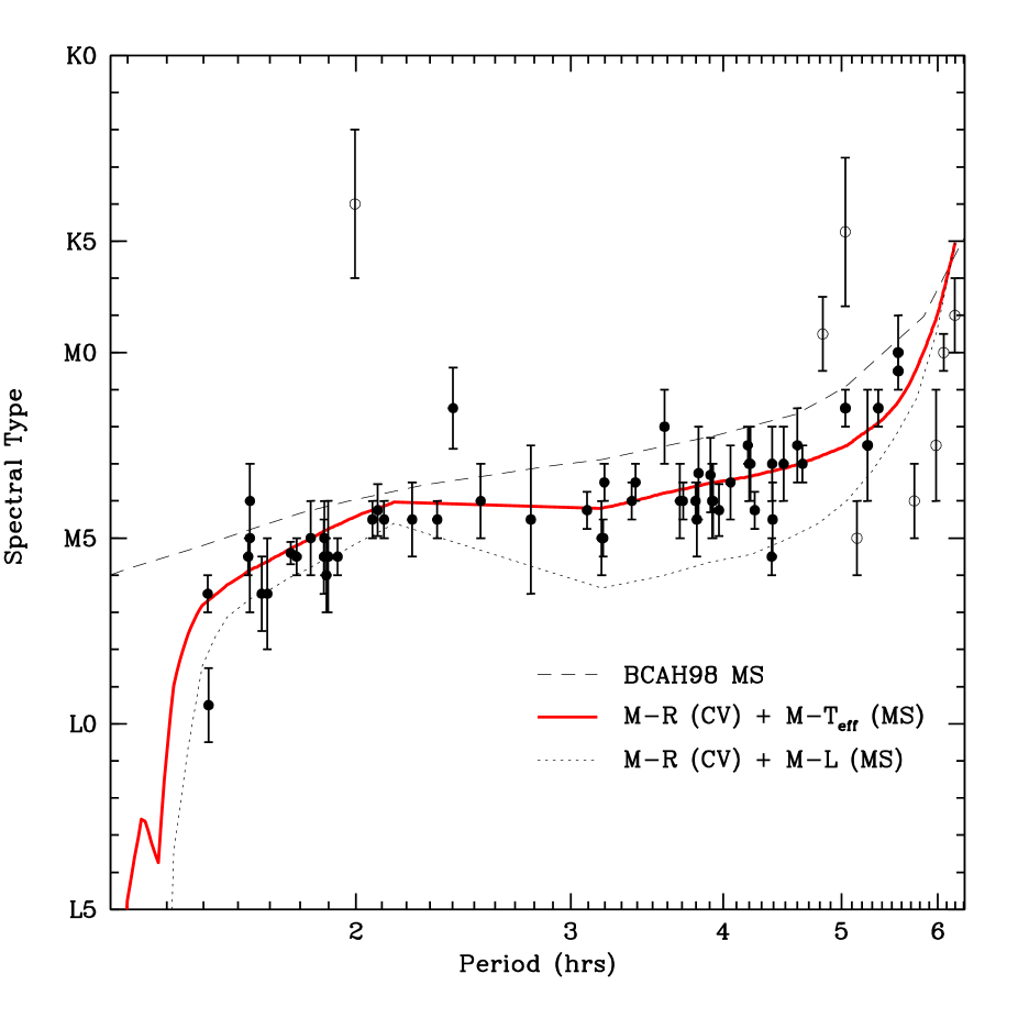
Figure 9: Observed vs predicted spectral types of CV donors. Points correspond to empirically determined $SpT$s for CVs with $P_{orb}\raisebox{-2.58334pt}{$\;\stackrel{{\scriptstyle\raisebox{-0.60275pt}{$\textstyle<$}}}{{\sim}}\;$}6$ hrs, taken from Table 2. Likely evolved donors are shown as open symbols and were excluded from the statistics quoted in the text. The solid red line shows the $SpT$($P_{orb}$) relation predicted by the semi-empirical donor sequence. The dashed line shows the relation predicted by the BCAH98 5 Gyr isochrone. The dotted line shows the relation that would be obtained if CV donors obeyed the MS mass-luminosity relation, rather than the MS mass-effective temperature relation. The kinks in the solid and dotted lines are due to a switch between two different model atmosphere grids.

It is worth stressing that the predicted sequence is not a fit to the data, i.e. the good match between predicted and observed $SpT$s has been achieved without any adjustable parameters. What this means is that the empirical $M_{2}-R_{2}$ relation yields just the right amount of radius expansion to account for the late spectral types of the donors. Thus the results of P05 and B98 are mutually consistent.

We also show in Figure 9 the donor sequence that would result if we had adopted the MS mass-luminosity relation for CV donors (rather than the correct mass-effective temperature one). As expected, this predicts even later spectral types, since in this case the bloated donor must reduce its $T_{eff}$ in order to maintain the MS luminosity that would be appropriate for its mass. This sequence does not match the data nearly as well – the average offset from the data is 1.4 spectral sub-types – but it does provides a useful lower limit on the predicted $SpT$s.

We finally comment again on the remarkably small scatter in the $SpT$-$P_{orb}$ diagram for unevolved CVs. In principle, we could try to estimate the intrinsic dispersion demanded by the data in the same way as in Section 2.3, i.e. by demanding that $\chi^{2}_{\nu}=1$ for the correct $\sigma_{int,SpT}$. This would yield $\sigma_{int,SpT}\simeq 0.4$. However, this value should perhaps not be taken at face value, since most spectral type errors are ad hoc estimates that cannot be expected to be Gaussian or even strictly 1-$\sigma$. A more robust statement is that the average intrinsic dispersion must be less than the RMS scatter of about 1 spectral sub-type. This is still quite impressive: in the M-dwarf regime, one sub-type typically spans an effective temperature range of only $\Delta T_{eff}\simeq 100-250$ K.

4.3 Applying the Donor Sequence: Distances from Photometric Parallaxes

We conclude our study by exploring one obvious practical application of the semi-empirical donor sequence, namely distance estimation. Distances towards CVs are of fundamental importance to virtually all areas of CV research, but are notoriously difficult to determine. In recent years, trigonometric parallaxes have finally been determined for a number of systems, but indirect methods remain the only way to obtain distance estimates for the vast majority of CVs.

Perhaps the most widely used indirect technique for estimating distances towards CV is Bailey’s (1981) method. This is based on the K-band surface brightness ($S_{K}$) of the secondary, defined as

$$S_{K}=K+5-5\log{d}+5\log{R_{2}/R_{\odot}}$$ (14)

where $d$ is the distance in parsecs. $S_{K}$ can be calibrated against colour (usually $(V-K)$) by using a suitable sample of MS stars. The distance towards a CV can then be estimated if the apparent K-band magnitude, $V-K$ colour and radius of the donor are known. In practice, the K-band magnitude of the CV is usually assumed to be dominated by the donor (so the resulting distance estimate is really a lower limit). Also, the radius is generally estimated from the orbital period, by using the $P_{orb}$-$\rho_{2}$ relation (Equation 3) and assuming a MS mass-radius relation. However, the most difficult aspect of the method is the determination of an appropriate $V-K$ value for the secondary, since the optical flux of CVs is usually dominated by accretion light.

Given this difficulty, much of the original promise of Bailey’s method derived from the form he inferred for the $S_{K}(V-K)$ relation. He found that for M-dwarfs (and thus for almost all CV donors), $S_{K}$ was essentially constant, so that even large errors in $V-K$ would not seriously affect the resulting distance estimates. However, the $S_{K}(V-K)$ relation has since been recalibrated by Ramseyer (1994), B99 and, most importantly, Beuermann (2000). The last of these studies provides by far the cleanest calibration to date and shows definitively that $S_{K}$ is not constant in the M-dwarf regime. Instead, the $S_{K}(V-K)$ relation is approximately linear over essentially the full range of $SpT$s found in CVs. As a result, Bailey’s original method is much less robust than had previously been supposed, unless the contribution of the donor to both V and K band fluxes can be estimated reliably from observations. This is usually impossible, and the only way forward is then to assume a “typical” donor $(V-K)$ for any given CV, based perhaps on its observed $SpT$ or just on its orbital period.

Our semi-empirical donor sequence provides a way to simplify and improve such distance estimates. As already noted above, the small scatter around the $M_{2}-R_{2}$ and the $SpT-P_{orb}$ relations implies that most CVs do, in fact, follow the unique evolution track that is delineated by this sequence. We can therefore use the absolute magnitudes predicted along the sequence to obtain lower limits on the distance towards any CV, under the single assumption that the system follows the standard track. For example, the lower limit on the distance associated with a single epoch $K$-band measurement is

$$\log{d_{lim}}=\frac{K-M_{K,2}(P_{orb})+5}{5},$$ (15)

where $K$ is the apparent magnitude and $M_{K,2}$ is the absolute $K$-band magnitude on the donor sequence at the CV’s orbital period. In principle, the apparent magnitude should be extinction-corrected, but in practice this correction is usually negligible for CVs in the infrared. If the donor contribution to the total flux is known, the apparent magnitude of the system should of course be replaced with that of the donor to yield an actual estimate of the distance (rather than just a lower limit).

In order to test this method, we have compiled distances and 2MASS infrared magnitudes for all CV with trigonometric parallax measurements. The sample is listed in Table 4 and contains 23 systems, 22 of which have reliable 2MASS measurements. In Figure 10, the absolute JHK magnitudes are shown as a function of orbital period and compared to the predictions for the donor stars from the semi-empirical sequence in Table 3. We have intentionally not corrected the observed data points for interstellar extinction. In practical applications, extinction estimates will often not be available, and our main goal here is to test how well distances may be estimated just from single-epoch infrared magnitudes and orbital periods. Extinction estimates are nevertheless listed in Table 4 and are negligible for the sources in our sample.

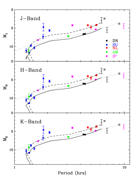
Figure 10: Infrared absolute magnitudes of CVs as a function of $P_{orb}$. Points correspond to absolute magnitudes for CVs with trigonometric parallaxes and reliable 2MASS observations (Table 4). Colours correspond to various CV sub-types, as indicated (DN = dwarf nova; SU = SU UMa star; NL = non-magnetic nova-like; AM = AM Her star; IP = intermediate polar). Systems with $P_{orb}>6$ hrs are shown as open symbols. Solid lines show the tracks predicted by the semi-empirical donor sequence, and dotted lines show the tracks corresponding to the BCAH98 5 Gyr isochrone. The dashed lines show the CV donor tracks offset by the average offset between the data points and the pure donor predictions; see text for details.

Perhaps the most important point to note from Figure 10 is that the semi-empirical donor sequence does a nice job of tracing the lower envelope of the data points. No CV with $P_{orb}<6$ hrs is significantly fainter in the infrared than the donor prediction. This again validates the sequence and implies that it can be used with confidence to determine lower limits on CV distances. However, it is also obvious from Figure 10 that the majority of systems are significantly brighter than the pure donor prediction, even in the K-band. Thus in most CVs, even the infrared flux is dominated by accretion light (cf. Dhillon et al. 2000).

We have determined the average offsets between the donor sequence and the data in the three infrared bands, for systems with $P_{orb}<6$ hrs. In doing so, we assumed that none of the systems in our sample are period bouncers, except WZ Sge, which was removed from the sample for the purpose of this calculation. The resulting offsets are

$$\begin{array}[]{ll}\Delta J=1.56&\sigma_{\Delta J}=1.25,\\ \Delta H=1.34&\sigma_{\Delta J}=1.12,\\ \Delta K=1.21&\sigma_{\Delta J}=1.07,\end{array}$$ (16)

where $\sigma_{\Delta JHK}$ is the scatter of the data around the mean offsets. As one might expect, both the offsets and the scatter decrease with increasing wavelength. However, even at $K$, the donor typically contributes only 33% of the total flux. The corresponding contributions at J and H are 24% and 29%, respectively. Thus a distance limit obtained from a single epoch infrared measurement with no additional information would typically underestimate the true distance by factors of 2.05 (J), 1.86 (H) and 1.75 (K).

If it was deemed important to convert these robust lower limits into (much less robust) distance estimates, one might consider applying the mean offsets to the absolute donor magnitudes. We hasten to emphasize that this procedure has no physical basis, and indeed there is no reason to think a priori that a single offset should yield reasonable results across the full range of orbital periods and CV types. Nevertheless, the effect of applying these offsets to the donor sequence is illustrated in Figure 10 (dashed lines). The $\sigma_{JHK}$ values indicate that, for our sample, the resulting distance estimates would be correct to about a factor of 1.78 (J), 1.68 (H) and 1.64 (K).

Table 4: Distance moduli and absolute infrared magnitudes for CVs with trigonometric parallaxes. Apparent magnitudes were taken from the final 2MASS catalog and converted to the CIT system using the transformations given by Carpenter (2001). Note that HV Vir has a parallax but no reliable 2MASS detection. Note that any asymmetric errors on the distance moduli have been symmetrized for simplicity; see the original references for the exact uncertainties. We also provide estimated reddening values ($E_{B-V}$) from Verbunt (1987). For reference, the associated extinctions are $A_{J}=0.89\times E_{B-V}$, $A_{H}=0.43\times E_{B-V}$ and $A_{K}=0.35\times E_{B-V}$ (Rieke & Lebofsky 1985). All systems that are not included in Verbunt (1987) are very close and are therefore listed here with reddening entries of (0.0). The distance references indicated in the last column are 1 = Duerbeck (1999); 2 = Harrison et al. (2004); 3 = Thorstensen (2003); 4 = McArthur et al. (1999); 5 = McArthur et al. (2001); 6 = Beuermann et al. (2004); 7 = Beuermann et al. (2003).

System	$P_{orb}(hrs)$	Type	$m-M$	$M_{J}$	$M_{H}$	$M_{K}$	$E_{B-V}$	Ref
AE Aqr	9.880	DQ	5.04 $\pm$ 0.65	4.42 $\pm$ 0.65	3.87 $\pm$ 0.65	3.76 $\pm$ 0.65	(0.00)	1
RU Peg	8.990	DN/UG	7.29 $\pm$ 0.17	3.78 $\pm$ 0.17	3.33 $\pm$ 0.17	3.20 $\pm$ 0.17	0.00	2
Z Cam	6.956	DN/ZC	6.06 $\pm$ 0.67	5.51 $\pm$ 0.67	4.98 $\pm$ 0.67	4.82 $\pm$ 0.67	0.00	3
SS Cyg	6.603	DN/UG	6.13 $\pm$ 0.15	2.41 $\pm$ 0.15	2.22 $\pm$ 0.15	2.19 $\pm$ 0.15	0.04	2
AH Her	6.195	DN/ZC	9.10 $\pm$ 0.76	2.89 $\pm$ 0.76	2.63 $\pm$ 0.76	2.58 $\pm$ 0.76	0.03	3
RW Tri	5.565	NL	7.79 $\pm$ 0.22	4.16 $\pm$ 0.22	3.78 $\pm$ 0.22	3.69 $\pm$ 0.22	0.10	4
TV Col	5.486	IP	7.87 $\pm$ 0.10	5.34 $\pm$ 0.10	4.95 $\pm$ 0.10	4.85 $\pm$ 0.10	0.00	5
V3885 Sgr	4.971	NL	5.21 $\pm$ 0.48	4.76 $\pm$ 0.48	4.52 $\pm$ 0.48	4.43 $\pm$ 0.48	0.00	1
IX Vel	4.654	NL	4.91 $\pm$ 0.20	4.23 $\pm$ 0.20	4.06 $\pm$ 0.20	3.94 $\pm$ 0.20	0.00	1
SS Aur	4.387	DN/UG	6.13 $\pm$ 0.13	6.57 $\pm$ 0.13	6.13 $\pm$ 0.13	5.89 $\pm$ 0.13	0.10	2
U Gem	4.246	DN/UG	5.01 $\pm$ 0.09	6.63 $\pm$ 0.09	6.05 $\pm$ 0.09	5.84 $\pm$ 0.09	0.00	2
V1223 Sgr	3.366	IP	8.61 $\pm$ 0.20	4.23 $\pm$ 0.20	4.12 $\pm$ 0.20	4.05 $\pm$ 0.20	0.15	6
AM Her	3.094	AM	4.49 $\pm$ 0.19	7.21 $\pm$ 0.19	6.70 $\pm$ 0.19	6.54 $\pm$ 0.19	(0.00)	3
YZ Cnc	2.083	DN/SU	7.54 $\pm$ 0.29	5.64 $\pm$ 0.29	5.40 $\pm$ 0.29	5.31 $\pm$ 0.29	0.00	2
SU UMa	1.832	DN/SU	7.07 $\pm$ 1.06	4.73 $\pm$ 1.06	4.65 $\pm$ 1.06	4.62 $\pm$ 1.06	0.00	3
V893 Sco	1.823	DN/SU	5.95 $\pm$ 0.61	7.28 $\pm$ 0.61	6.95 $\pm$ 0.61	6.75 $\pm$ 0.61	(0.00)	3
EX Hya	1.638	IP	4.05 $\pm$ 0.04	8.23 $\pm$ 0.05	7.89 $\pm$ 0.05	7.66 $\pm$ 0.05	0.00	7
VY Aqr	1.514	DN/SU/WZ	4.93 $\pm$ 0.30	10.34 $\pm$ 0.30	9.91 $\pm$ 0.31	9.68 $\pm$ 0.31	(0.00)	3
T Leo	1.412	DN/SU	5.02 $\pm$ 0.26	9.74 $\pm$ 0.26	9.30 $\pm$ 0.26	8.83 $\pm$ 0.26	(0.00)	3
HV Vir	1.370	DN/SU/WZ	8.31 $\pm$ 1.37	–	–	–	–	3
WZ Sge	1.361	DN/SU/WZ	3.19 $\pm$ 0.14	11.66 $\pm$ 0.15	11.35 $\pm$ 0.15	10.83 $\pm$ 0.15	0.00	2
EF Eri	1.350	AM	6.06 $\pm$ 0.77	11.09 $\pm$ 0.80	9.60 $\pm$ 0.78	9.33 $\pm$ 0.79	(0.00)	3
GW Lib	1.280	DN/SU/WZ	5.09 $\pm$ 0.51	11.10 $\pm$ 0.51	10.49 $\pm$ 0.52	10.33 $\pm$ 0.54	(0.00)	3

5 Discussion and Conclusions

The main goal of this paper has been the construction of a complete, semi-empirical donor sequence for CVs that is based on our best understanding of donor properties and is consistent with all key observational constraints. This donor sequence is provided in Table 3 and is based primarily on an updated version of the mass-radius relationship for CV secondaries determined by P05. It also relies on a MS-based mass-effective temperature relation that has been shown to be appropriate for CV donors by theoretical work, and on up-to-date stellar atmosphere models. By design, the donor track also reproduces the observed locations of the period gap and the period minimum, and extends beyond this to the period bouncer regime. We have shown that this sequence provides an excellent match to the observed $SpT$-$P_{orb}$ relation for unevolved CV donors (i.e. $P_{orb}\raisebox{-2.58334pt}{$\;\stackrel{{\scriptstyle\raisebox{-0.60275pt}{$\textstyle<$}}}{{\sim}}\;$}6$ hrs), and that it correctly traces the lower envelope of the $M_{JHK}-P_{orb}$ distributions of CVs.

Along the way, we have revisited and updated two important results on CV donors by P05 and B98. Regarding the former study, we have carried out a full, independent analysis of the superhumper and eclipser data that was used by P05 to construct their empirical $M_{2}-R_{2}$ relation. We constructed and used our own $q-\epsilon$ calibration for superhumpers, verified the validity of the constant $M_{1}$ assumption on which the method rests, imposed the locations of the period gap and the period minimum as constraints on the mass-radius relation and used a self-consistent fitting technique to extract optimal parameters for the $M_{2}-R_{2}$ relations for long-period CVs, short-period CVs and period-bouncers.

Regarding the study by B98, we have updated their $SpT$ data base for CV secondaries. Our new sample contains 91 CV donors with spectroscopically-determined $SpT$ estimates (compared to 54 donors in the B98 sample). Comparing the $SpT$-$P_{orb}$ distribution to that of MS stars, we find that CV donors have later spectral types at all orbital periods. This extends the finding of B98 to the short-period regime ($P_{orb}\raisebox{-2.58334pt}{$\;\stackrel{{\scriptstyle\raisebox{-0.60275pt}{$\textstyle<$}}}{{\sim}}\;$}3$ hrs).

We find that there is remarkably little intrinsic scatter about both the mean $M_{2}-R_{2}$ and $SpT-P_{orb}$ relations for CVs with $P_{orb}<6$ hrs: probably no more than a few percent in $R_{2}$ and less than 1 spectral sub-type. This suggests that, on long time-scales, most CVs do indeed follow a unique evolution track, just as is theoretically expected (e.g. Kolb 1993; Stehle, Ritter & Kolb 1996). The large scatter in luminosity-based accretion rate estimates at fixed $P_{orb}$ (e.g. Patterson 1984) is therefore probably caused by fluctuations around the mean mass transfer rate on time-scales that are short compared to the time-scale on which the donor loses mass and the binary evolves (see Büning & Ritter 2004 and references therein). In principle, the empirical $M_{2}-R_{2}$ relationship for CV donors can be inverted to infer the long-term average mass-transfer rate as a function of orbital period; this will be the subject of a separate paper.

An important feature of our donor sequence is a sharp decline in effective temperature, luminosity and optical/IR brightness, well before the period minimum is reached. In fact, the L/T transition essentially coincides with $P_{min}$ on the evolution track (although this statement depends somewhat on the validity of our spectral type calibration in a sparsely populated regime). Beyond $P_{min}$, even the accretion-heated WD alone is expected to outshine the donor at optical wavelengths and it is comparably bright to the donor even in the infrared. All of this helps to explain why brown dwarf donors have proven so difficult to detect in CVs, especially in suspected period bouncers.

Finally, we have looked at one obvious application of our donor sequence, the determination of distance estimates from infrared photometry. We have shown that robust lower limits can indeed be obtained, but that, in our calibration sample, these are typically a factor of two smaller than the true distances. Thus, even in the infrared, the donor typically contributes only $\simeq$30% of the total flux. Distance estimates that explicitly allow for this average donor contribution are typically good to about a factor of 2 in our calibration sample.

Appendix A Calibrating the $\epsilon-q$ Relation

Here we provide some additional details on the way in which we calibrated the $\epsilon-q$ relation. As already noted in Section 2.2, we rely on the same calibrators as P05 (given in their Table 7), but there are a few differences between their treatment of the problem and ours. First, the two calibrators with the most precise mass ratios are XZ Eri and DV UMa (Feline et al. 2004). In both cases, Feline et al. obtained their final $q$-estimates as weighted averages over the mass ratios determined in 3 different photometric bands. However, we found the individual $q$-estimates for both systems were not quite consistent at the level expected based on their internal errors. We therefore re-averaged the individual $q$ values, but allowed explicitly for just enough intrinsic dispersion to make the values in all bands consistent with each other. The resulting new mass ratios were $q=0.111\pm 0.03$ (XZ Eri) and $q=0.152\pm 0.003$ (DV UMa). The implied changes to the mass ratios are relatively small, but the increase in the formal errors is important (since these two data points would otherwise be given too much weight in the calibration). Second, we took note of the approximate upper limit on the mass ratio of BB Dor suggested by P05 ($q<0.38$), but did not explicitly enforce it in our fits. Instead, we decided to check a posteriori if our fits significantly violated this approximate constraint or not. Third, we chose to treat $q$ (rather than $\epsilon$) as the independent variable of the problem, since the ultimate goal is to estimate $q$ from a measured $\epsilon$. Fourth, we experimented with a variety of different families of 2-parameter curves, including linear fits (with constant term), quadratic fits (with no constant term) and power laws.

We found that the preferred functional form for the $\epsilon-q$ relation is linear, i.e. $q=a+b\epsilon$, with $a$ and $b$ constants. We obtained optimal estimates of $a$ and $b$ by minimizing the $\chi^{2}$ of the model with respect to the data, allowing explicitly for errors in both $q$ and $\epsilon$ and also for the possibility of intrinsic scatter around the relation, $\sigma_{int}$. The goodness-of-fit metric then becomes

$$\chi^{2}=\sum_{i=1}^{N}\frac{(q-a-b\epsilon)^{2}}{\sigma^{2}_{q}+b^{2}\sigma_{\epsilon}^{2}+\sigma_{int}^{2}}.$$ (17)

The $\epsilon-q$ relation given in the main body is the minimum $\chi^{2}$ solution. It does not significantly violate the approximate upper limit on BB Dor’s mass ratio and achieves a statistically acceptable $\chi^{2}_{\nu}=1.03$ with $\sigma_{int}=0$. Thus any intrinsic scatter around the calibrating relation must be small compared to the statistical errors on the data point. P05 explicitly added an extra 5% uncertainty on both $q$ and $\epsilon$ when carrying out their fits. We appreciate their rationale for doing this (allowing for variability in superhump periods and unaccounted-for external errors in published mass ratio estimates); indeed, we accounted for the possibility of a non-zero $\sigma_{int}$ in our fits for exactly the same reasons. However, it simply turns out that such additional error contributions are not actually demanded by the data.

Appendix B Testing the Assumption of Constant Primary Mass

In order to test if there is evidence for evolution of $M_{1}$, we fitted a straight line to the $N=16$ eclipser data points with $P_{orb}<6$ hrs given in Table 7 in P05. Orbital period errors are negligible compared to the errors on $M_{1}$ and to the intrinsic dispersion, so we used the $\chi^{2}$ metric

$$\chi^{2}=\sum_{i=1}^{N}\frac{(M_{1}-a-bP_{orb})^{2}}{\sigma^{2}_{M_{1}}+\sigma^{2}_{int}}.$$ (18)

Here, $\sigma_{M_{1}}$ is the error on $M_{1}$ and $\sigma_{int}$ is the intrinsic dispersion around the fit. The intrinsic dispersion is set to the value needed to obtain a reduced $\chi^{2}_{\nu}\simeq 1$, where $\nu=N-2$; for the linear fit, this value is $\sigma_{int}=0.16M_{\odot}$. The corresponding constraints on the slope and intercept are shown in the top panel of Figure 2, and the best-fitting line itself is plotted in the bottom panel. There is certainly substantial scatter among the $M_{1}$ values, but the best-fitting slope is not significantly different from zero. Thus there is no convincing evidence for a trend of $M_{1}$ with $P_{orb}$. The best-fitting constant $M_{1}$, using the same $\chi^{2}$ metric, but with slope fixed at $b=0$, yields a mean WD mass of $M_{1}=0.75\pm 0.05M_{\odot}$. It requires the same level of intrinsic scatter as the linear fit, i.e. $\sigma_{int}=0.16M_{\odot}$.

These results may seem at odds with the studies of Webbink (1990) and Smith & Dhillon (1998), both of whom suggested that CVs below the gap tend to have lower WD masses than those above the gap. More specifically, Smith & Dhillon [Webbink] derived weighted mean masses of $M_{1}=0.66\pm 0.01M_{\odot}$ [$0.66\pm 0.01M_{\odot}$] below the gap a nd $M_{1}=0.78\pm 0.02M_{\odot}$ [$0.81\pm 0.04M_{\odot}$] above the gap. Two points are important to note here. First, the weights that were used in calculating these weighted means were the inverse variances of the formal errors on the individual data points. Second, the quoted uncertainties on the means are the formal errors on the weighted means, rather than the dispersion of the points around the means. If we calculate the same quantities for our sample (in which there are 8 short- and 8 long-period systems), we find weighted means with formal errors of $M_{1}=0.642\pm 0.007M_{\odot}$ below the gap and $M_{1}=0.72\pm 0.02M_{\odot}$ above the gap. So if we had used these measures, there would appear to be a significant difference between short- and long-period systems for our sample, too.

The resolution of this apparent paradox is simple. As already noted by Smith & Dhillon, the weighted means and their formal errors are quite misleading, since they can be totally dominated by a few systems with small formal uncertainties. If the true intrinsic dispersion among the sample being averaged is larger than these formal uncertainties – as it clearly is here – then the formal error on the weighted mean (and even the weighted mean itself) is rather meaningless. From a statistical point of view, such a sample violates the basic premise underlying the calculation of the weighted mean, which is that each data point is drawn from a distribution with the same mean, with a variance given solely by the formal error.

Smith & Dhillon also give the unweighted means and dispersions for their sample, which are $M_{1}=0.69\pm 0.13M_{\odot}$ below the gap and $M_{1}=0.80\pm 0.22M_{\odot}$ above the gap. For our sample, the corresponding numbers are $M_{1}=0.74\pm 0.20M_{\odot}$ below the gap and $M_{1}=0.78\pm 0.16M_{\odot}$ above the gap. This already shows that the differences between short- and long-period systems are much less significant than suggested by the formal weighted means and errors, and that any real trend with $P_{orb}$ that might be present is small compared to the intrinsic dispersion.

However, the best way to estimate the means, error on the means and intrinsic dispersion is via the statistic given by Equation 18 (again with slope fixed at $b=0$). This accounts explicitly for both the formal errors and intrinsic dispersion, with the latter being adjusted to yield a reasonable $\chi^{2}_{\nu}$. If we do this separately for short- and long-period systems in our sample, we find $M_{1}=0.73\pm 0.07M_{\odot}$ with $\sigma_{int}=0.19M_{\odot}$ below the gap and $M_{1}=0.77\pm 0.06M_{\odot}$ with $\sigma_{int}=0.15M_{\odot}$ above the gap. As expected, these numbers are not significantly different from each other anymore.

Appendix C Fitting the $M_{2}-R_{2}$ Relation

We wish to obtain an optimal estimate of the mass-radius relation of CV donors from a set of ($M_{2},R_{2}$) pairs. As noted in Section 2.5, the key challenges are to acccount for the correlated nature of the errors on $M_{2}$ and $R_{2}$ and to self-consistently impose the external constraints derived from the locations of the period gap and the period minimum. In addition, we also need to allow for intrinsic scatter around the mass-radius relation.

We begin by defining the analytical form of the mass-radius relation we wish to fit to the data. Based on inspection of the data in Figure 3, we will follow P05 and describe the mass-radius relation as a power law,

$$\frac{R_{mod}}{R_{ref}}=\left(\frac{M}{M_{ref}}\right)^{b}.$$ (19)

Here and below, we drop the subscript “2” on the mass and radius in order to keep the notation transparent. In practice, we carry our fits out in log-space, where the power law transforms into the linear relation

$$\log{R_{mod}}=\log{R_{ref}}\;+b\log{M}\;-b\log{M_{ref}}.$$ (20)

In the absence of additional constraints, both $R_{ref}$ and $b$ would be free parameters of this model. However, as discussed in Section 2.4, we will demand that $M=M_{conv}$ at $P_{orb}=P_{gap,\pm}$ and $M=M_{bounce}$ at $P_{orb}=P_{min}$. The easiest way to accomplish this is to adopt $M_{ref}=M_{conv}$ for long- and short-period CVs and $M_{ref}=M_{bounce}$ for period bouncers. With these choices of reference mass, $R_{ref}$ is fixed (to within some error) by the period-density relation for Roche-lobe filling stars (Equation 6). Thus for long period CVs, we have

$$\begin{array}[]{l}\log{R_{ref}}=\log{0.2361R_{\odot}}\;+(2/3)\log{P_{gap,+}(hr)}+\\ \hskip 21.33955pt(1/3)\log{M_{conv}}\;-(1/3)\log{M_{\odot}}.\end{array}$$ (21)

Similar relations hold for short-period CVs and period bouncers. Note that in all these relations, $P_{gap,\pm}$(or $P_{min}$) and $M_{conv}$ (or $M_{bounce}$) are empirical estimates with associated unertainties. As discussed further below, these uncertainties translate into a systematic error on each data point that needs to be accounted for in the final fit.

However, let us first deal with the correlation between the $M$ and $R$ estimates for a given system. The easiest way to achieve this is to work exclusively in terms of $M$. For example, consider a particular data point ($M_{i}$, $R_{i}$, $P_{orb,i}$) in the short-period regime (the corresponding derivation for long-period systems and period bouncers is identical). The residual between this point and the model prediction is $\Delta_{i}=\log{R_{i}}-\log{R_{mod,i}(M_{i})}$. Using Equations 6,  19 and 21, this can be rewritten as

$$\begin{array}[]{l}\Delta_{i}=\frac{2}{3}\log{P_{orb,i}}\;-\frac{2}{3}\log{P_{gap,-}}+\\ \hskip 21.33955pt\left(\frac{1}{3}-b\right)\log{M_{i}}\;-\left(\frac{1}{3}-b\right)\log{M_{conv}}.\end{array}$$ (22)

Let us ignore the systematic errors arising from the uncertainties on $M_{conv}$ and $P_{gap,-}$ for the moment and consider only the statistical variance on $\Delta_{i}$. This is

$$\sigma_{stat,i}^{2}=\left(\frac{1}{3}-b\right)^{2}$$ (23)

where we have neglected the error on $P_{orb,i}$ which is always much smaller than that on $M_{i}$. An optimal estimate for $b$ could then be obtained by minimizing the usual $\chi^{2}$ statistic

$$\chi^{2}=\sum_{i=1}^{N}\frac{\Delta_{i}^{2}}{\sigma_{stat,i}^{2}},$$ (24)

or, if we additionally want to allow for an intrinsic variance $\sigma_{int}^{2}$,

$$\chi^{2}=\sum_{i=1}^{N}\frac{\Delta_{i}^{2}}{\sigma_{stat,i}^{2}+\sigma_{int}^{2}},$$ (25)

where $N$ is the number of data points.

We should also face up to the uncertainties on $M_{conv}$ and $P_{gap,-}$. It is tempting to simply account for these in the denominator of Equation 25. However, this would be incorrect, since any change in these quantities affects all residuals in the same way: $\sigma_{\log{M}_{conv}}$ and $\sigma_{\log{P}_{gap,-}}$ are systematic errors in this context. Let us define the systematic variance on each residual as

$$\sigma_{sys}^{2}=\frac{4}{9}\sigma_{\log{P}_{gap,-}}^{2}\;+\;\left(\frac{1}{3}-b\right)^{2}\sigma_{\log{M_{conv}}}^{2}.$$ (26)

It is then possible to define a new $\chi^{2}$ statistic that has the correct distribution and accounts for both $\sigma_{stat,i}$ and $\sigma_{sys}$. Following Stump et al. (2002), we find that in our case, this statistic is

$$\chi^{2}=\sum_{i=1}^{N}\frac{\Delta_{i}^{2}}{\sigma_{stat,i}^{2}+\sigma_{int}^{2}}\;-\;\frac{\left[\sum_{i=1}^{N}\frac{\Delta_{i}\sigma_{sys}}{\sigma_{stat,i}^{2}+\sigma_{int}^{2}}\right]^{2}}{1+\sum_{i=1}^{N}\frac{\sigma_{sys}^{2}}{\sigma_{stat,i}^{2}+\sigma_{int}^{2}}}.$$ (27)

The only uncertainties we have not explicitly accounted for in our fits are (i) the error on the mean white dwarf mass adopted for superhumpers and (ii) the errors on the parameters of the $\epsilon-q$ calibration. As discussed in Sections 2.3 and 2.2, these uncertainties also translate into systematic errors on the data points. In principle, it would be possible to formally account for these systematics in a similar way as we just did for the errors on $P_{gap,\pm}$ and $M_{conv}$, for example. However, in practice, such a treatment would be considerably more difficult and (in our view) a little pointless. The added difficulty arises partly because these new systematics do not affect all data points in a given mass/period regime (i.e. only the superhumpers, but not the eclipsers); the error on the calibration parameters, in particular, does not even affect all superhumpers in the same way. We feel the additional complexity this would introduce is not warranted. After all, regarding (i), we already know that the error on the mean $M_{1}$ is small compared to intrinsic dispersion around this mean, which we do account for (see Section 2.3). And regarding (ii), we already noted in Section 2.2 that the systematic uncertainty associated with the $\epsilon-q$ relation is small in the well-calibrated regime, but not necessarily well-described by the formal parameter uncertainties in the poorly-calibrated regime. Rather than attempt to include this poorly defined systematic in our fits, we thus prefer to simply emphasize its existence.

The optimal estimate of the power-law exponent $b$ is obtained by minimizing Equation 27. For long- and short-period systems, we determine the appropriate level of $\sigma_{int}$ by requiring that the reduced $\chi^{2}$ should be equal to one; for period bouncers, the reduced $\chi^{2}$ is slightly less than one even without any intrinsic dispersion. However, this is probably more of a reflection of the sparseness of the data in this regime than of any true constraint on $\sigma_{int}$. We therefore conservatively adopt the value of $\sigma_{int}$ obtained for short-period CVs for the period bouncers as well. Errors on the power law exponents can be estimated in the usual way. For example, the 1-$\sigma$ confidence interval around $b$ corresponds to the range of exponents for which $\chi^{2}\leq\chi^{2}_{min}+1$, where $\chi^{2}_{min}$ is the lowest value of $\chi^{2}$.

In order to test this method, we have carried out Monte Carlo simulations. Thus we created fake data sets with known slopes and subject to all of the errors we are trying to account for in our fits. In these simulations, the method did a good job in recovering the correct slope, and the distribution of the recovered slopes had a dispersion consistent with the estimated error on the slope.

References

- [Allard et al.(2000)] Allard, F., Hauschildt, P. H., & Schwenke, D. 2000, ApJ, 540, 1005
- [Allard et al.(2001)] Allard, F., Hauschildt, P. H., Alexander, D. R., Tamanai, A., & Schweitzer, A. 2001, ApJ, 556, 357
- [Bailey(1981)] Bailey, J. 1981, MNRAS, 197, 31
- [Baraffe et al.(1998)] Baraffe, I., Chabrier, G., Allard, F., & Hauschildt, P. H. 1998, A&A, 337, 403
- [\citeauthoryearBaraffe & Kolb2000] Baraffe I., Kolb U., 2000, MNRAS, 318, 354
- [Baraffe et al.(2002)] Baraffe, I., Chabrier, G., Allard, F., & Hauschildt, P. H. 2002, A&A, 382, 563
- [Baraffe et al.(2003)] Baraffe, I., Chabrier, G., Barman, T. S., Allard, F., & Hauschildt, P. H. 2003, A&A, 402, 701
- [Bergeron et al.(1995)] Bergeron, P., Wesemael, F., & Beauchamp, A. 1995, PASP, 107, 1047
- [Bessell(1990)] Bessell, M. S. 1990, PASP, 102, 1181
- [Beuermann et al.(1998)] Beuermann, K., Baraffe, I., Kolb, U., & Weichhold, M. 1998, A&A, 339, 518
- [Beuermann et al.(1999)] Beuermann, K., Baraffe, I., & Hauschildt, P. 1999, A&A, 348, 524
- [Beuermann(2000)] Beuermann, K. 2000, New Astronomy Review, 44, 93
- [Beuermann et al.(2003)] Beuermann, K., Harrison, T. E., McArthur, B. E., Benedict, G. F., Gänsicke, B. T. 2003, A&A, 412, 821
- [Beuermann et al.(2004)] Beuermann, K., Harrison, T. E., McArthur, B. E., Benedict, G. F., Gänsicke, B. T. 2004, A&A, 419, 291
- [Büning & Ritter(2004)] Büning, A., & Ritter, H. 2004, A&A, 423, 281
- [Carpenter(2001)] Carpenter, J. M. 2001, AJ, 121, 2851
- [Chabrier et al.(2000)] Chabrier, G., Baraffe, I., Allard, F., & Hauschildt, P. 2000, ApJ, 542, 464
- [Delfosse et al.(2000)] Delfosse, X., Forveille, T., Ségransan, D., Beuzit, J.-L., Udry, S., Perrier, C., & Mayor, M. 2000, A&A, 364, 217
- [Dhillon et al.(2000)] Dhillon, V. S., Littlefair, S. P., Howell, S. B., Ciardi, D. R., Harrop-Allin, M. K., & Marsh, T. R. 2000, MNRAS, 314, 826
- [Duerbeck(1999)] Duerbeck, H. W. 1999, IBVS, 4731, 1
- [bla] Echevarría J. 1983, Rev.Mex.Astron.Astrof. 8, 109
- [Elias et al.(1982)] Elias, J. H., Frogel, J. A., Matthews, K., & Neugebauer, G. 1982a, AJ, 87, 1029
- [Elias et al.(1982)] Elias, J. H., Frogel, J. A., Matthews, K., & Neugebauer, G. 1982b, AJ, 87, 1893
- [Feline et al.(2004)] Feline, W. J., Dhillon, V. S., Marsh, T. R., & Brinkworth, C. S. 2004, MNRAS, 355, 1
- [\citeauthoryearFriend et al.1990] Friend M. T., Martin J. S., Connon-Smith R., Jones D. H. P., 1990a, MNRAS, 246, 637
- [\citeauthoryearFriend et al.1990] Friend M. T., Martin J. S., Connon-Smith R., Jones D. H. P., 1990b, MNRAS, 246, 654
- [Goodchild & Ogilvie(2006)] Goodchild, S., & Ogilvie, G. 2006, MNRAS, 368, 1123
- [Harrison et al.(2004)] Harrison, T. E., Johnson, J. J., McArthur, B. E., Benedict, G. F., Szkody, P., Howell, S. B., & Gelino, D. M. 2004, AJ, 127, 460
- [Hauschildt et al.(1999)] Hauschildt, P. H., Allard, F., & Baron, E. 1999, ApJ, 512, 377
- [Henry & McCarthy(1993)] Henry, T. J., & McCarthy, D. W., Jr. 1993, AJ, 106, 773
- [Kirkpatrick(2005)] Kirkpatrick, J. D. 2005, ARA&A, 43, 195
- [Kolb(1993)] Kolb, U. 1993, A&A, 271, 149
- [Kolb & Baraffe(1999)] Kolb, U., & Baraffe, I. 1999, MNRAS, 309, 1034
- [Kolb & Baraffe(2000)] Kolb, U., & Baraffe, I. 2000, New Astronomy Review, 44, 99
- [Kolb et al.(2001)] Kolb, U., King, A. R., & Baraffe, I. 2001, MNRAS, 321, 544
- [Leggett et al.(1996)] Leggett, S. K., Allard, F., Berriman, G., Dahn, C. C., & Hauschildt, P. H. 1996, ApJS, 104, 117
- [Leggett et al.(2001)] Leggett, S. K., Allard, F., Geballe, T. R., Hauschildt, P. H., & Schweitzer, A. 2001, ApJ, 548, 908
- [McArthur et al.(1999)] McArthur, B. E., et al. 1999, ApJl, 520, L59
- [McArthur et al.(2001)] McArthur, B. E., et al. 2001, ApJ, 560, 907
- [Mennickent et al.(2004)] Mennickent, R. E., Diaz, M. P., & Tappert, C. 2004, MNRAS, 347, 1180
- [Paczyński(1971)] Paczyński, B. 1971, ARA&A, 9, 183
- [Patterson et al.(2003)] Patterson, J., et al. 2003, PASP, 115, 1308
- [Patterson et al.(2005)] Patterson, J., et al. 2005, PASP, 117, 1204
- [\citeauthoryearPearson2006] Pearson K. J., 2006, MNRAS, 371, 235
- [Podsiadlowski et al.(2003)] Podsiadlowski, P., Han, Z., & Rappaport, S. 2003, MNRAS, 340, 1214
- [Ramseyer(1994)] Ramseyer, T. F. 1994, ApJ, 425, 243
- [Rappaport et al.(1983)] Rappaport, S., Verbunt, F., & Joss, P. C. 1983, ApJ, 275, 713
- [Rieke & Lebofsky(1985)] Rieke, G. H., & Lebofsky, M. J. 1985, ApJ, 288, 618
- [Ritter & Kolb(2003)] Ritter, H., & Kolb, U. 2003, A&A, 404, 301
- [Smith & Dhillon(1998)] Smith, D. A., & Dhillon, V. S. 1998, MNRAS, 301, 767
- [Stehle et al.(1996)] Stehle, R., Ritter, H., & Kolb, U. 1996, MNRAS, 279, 581
- [Stump et al. (2002)] Stump, D et al. 2002, Phys. Rev. D, 65, 014012
- [Szkody et al.(2004)] Szkody, P., et al. 2004, AJ, 128, 1882
- [Thorstensen et al.(2002)] Thorstensen, J. R., Fenton, W. H., Patterson, J., Kemp, J., Halpern, J., & Baraffe, I. 2002a, PASP, 114, 1117
- [Thorstensen et al.(2002)] Thorstensen, J. R., Fenton, W. H., Patterson, J. O., Kemp, J., Krajci, T., & Baraffe, I. 2002b, ApJl, 567, L49
- [Townsley & Bildsten(2003)] Townsley, D. M., & Bildsten, L. 2003, ApJl, 596, L227
- [Verbunt(1987)] Verbunt, F. 1987, A&AS, 71, 339
- [Warner(1995)] Warner, B. 1995, ’Cataclysmic Variable Stars’, Cambridge Astrophysics Series, Cambridge, New York: Cambridge University Press
- [Thorstensen(2003)] Thorstensen, J. R. 2003, AJ, 126, 3017
- [Patterson(1984)] Patterson, J. 1984, ApJS, 54, 443
- [Webbink(1990)] Webbink, R. F. 1990, in Accretion-Powered Compact Binaries, Ed: C. W. Mauche, Cambridge: Cambridge University Press, p177,
- [Webbink & Wickramasinghe(2002)] Webbink, R. F., & Wickramasinghe, D. T. 2002, MNRAS, 335, 1