Cluster Disruption: Combining Theory and Observations

Abstract

We review the theory and observations of star cluster disruption. The three main phases and corresponding typical timescales of cluster disruption are: I) Infant Mortality ($\sim 10^{7}$ yr), II) Stellar Evolution ($\sim 10^{8}$ yr) and III) Tidal relaxation ($\sim 10^{9}$ yr). During all three phases there are additional tidal external perturbations from the host galaxy. In this review we focus on the physics and observations of Phase I and on population studies of Phases II & III and external perturbations (concentrating on cluster-GMC interactions). Particular attention is given to the successes and short-comings of the Lamers cluster disruption law, which has recently been shown to stand on a firm physical footing.

¹Department of Physics and Astronomy, University College London, Gower Street, London, WC1E 6BT, United Kingdom
²Astronomical Institute, Utrecht University, Princetonplein 5, NL-3584 CC Utrecht, The Netherlands

1. Introduction

The vast majority (perhaps all) of stars are formed in a clustered fashion. However, only a very small percentage of older stars are found in bound clusters. These two observations highlight the importance of clusters in the star-formation process and the significance of cluster disruption. The process of cluster disruption begins soon after, or concurrent with, cluster formation. Lada & Lada (2003) found that $\lesssim 10\%$ of stars formed in embedded clusters end up in bound clusters after $\sim 10^{8}$ yr. Whitmore (2003) and Fall et al. (2005) have shown that at least 20%, but perhaps all, star formation in the merging Antennae galaxies is taking place in clusters, the majority of which are likely to become unbound. The case is similar in M51, with $>60\%$ of all young ($<10$ Myr) clusters likely to be destroyed within the first 10s of Myr of their lives (Bastian et al. 2005). On longer timescales, Oort (1958) and Wielen (1971) noted a clear lack of older ($>$ few Gyr) open clusters in the solar neighbourhood and Boutloukos & Lamers (2003) found a strong absence of older clusters in M51, M33, SMC, and the solar neighbourhood.

The lack of old open clusters in the solar neighbourhood is even more striking when compared with the LMC, which contains a significant number of ‘blue globular clusters’ with ages well in excess of a Gyr (e.g. Gascoigne 1966; de Grijs & Anders 2006). This difference can be understood either as a difference in the formation history of clusters or as a difference in the disruption timescales. This later scenario was suggested by Hodge (1987), who directly compared the age distribution of Galactic open clusters and the SMC cluster population. He noted that there are $10-15$ times more clusters with an age of 1 Gyr in the SMC as compared to the solar neighbourhood (when normalising both populations to an age of $10^{8}$ yr) and concluded that disruption mechanisms must be less efficient in the SMC.

Much theoretical work has gone into the later scenario, with both analytic and numerical models of cluster evolution predicting a strong influence of the galactic tidal field on the dissolution of star clusters (for a recent review see Baumgardt 2006). Only recently has there been a large push to understand cluster disruption from an observational standpoint in various external potentials, making explicit comparison with models (Boutloukos & Lamers 2003; Lamers et al. 2005a, b; Gieles et al. 2005; Lamers & Gieles 2006).

We direct the reader to the review by Larsen in these proceedings for a historical look at the observations and theory of cluster disruption.

1.1. Phases of cluster disruption

While cluster disruption is a gradual process with several different disruptive agents at work simultaneously, one can distinguish three general phases of cluster mass loss and disruption. As we will see, a large fraction of clusters gets destroyed during the primary phase. The main phases and corresponding typical timescales of cluster disruption are: I) Infant Mortality ($\sim 10^{7}$ yr), II) Stellar Evolution ($\sim 10^{8}$ yr) and III) Tidal relaxation ($\sim 10^{9}$ yr). During all three phases there are additional tidal external perturbations from e.g. giant molecular clouds (GMCs), the galactic disc and spiral arms that heat the cluster and speed up the process of disruption. However, these external perturbations operate on longer timescales for cluster populations and so are most important in Phase III. In Fig. 1 we schematically illustrate the three Phases of disruption and the involved time-scales. Note that the number of disruptive agents decreases in time.

In this review we will focus on the physics and observations of Phase I as well as on recent population studies aimed at understanding Phases II and III on a statistical basis. For a recent review on the physics of Phases II and III, we refer the reader to Baumgardt (2006).

Figure 1.: Schematic overview of the three phases of cluster disruption considered and the responsible physics that drives the disruption.

Before proceeding, it is worthwhile to consider our definition of a cluster. Schweizer (2006) defines a cluster to be a gravitationally bound stellar association which will survive for 10–20 crossing times. This definition implies that the stars provide enough gravitational potential to bind the cluster and ignores the role of gas in the early evolution of clusters. In this review, we will define a cluster as a collection of gas and stars which was initially gravitationally bound. The reason for this definition will become evident in Section 2.

2. Infant Mortality

Recent studies on the populations of young star clusters in M51 (Bastian et al. 2005) and the Antennae galaxies (Whitmore 2003; Fall et al. 2005) have shown a large excess of star clusters with ages less than $\sim$10 Myr with respect to what would be expected assuming a constant cluster formation rate. The fact that open clusters in the solar neighbourhood display a similar trend (Lada & Lada 2003) has led to the conclusion that this is a physical effect and not simply that we are observing these galaxies at a special time in their star-formation history. If one adopts this view, then we are forced to conclude that the majority (between 60-90%) of star clusters become unbound when the remaining gas (i.e. gas that is left-over from the star formation process) is expelled. These clusters will survive less than a few crossing times.

2.1. Gas expulsion

Suppose that a star cluster is formed out of a sphere of gas with an efficiency $\epsilon$, where $\epsilon=M_{stars}/(M_{stars}+M_{gas})$. Further suppose that the gas and stars are initially in virial equilibrium. If we define the virial parameter as $Q=-2T/W$, with $T$ the kinetic energy and $W$ the potential energy, virial equilibrium implies $Q=1$. Finally, suppose that the remaining gas is removed on a timescale faster than the crossing time of stars in the cluster.

In such a scenario the cluster is left in a super-virial state after the gas removal, with $Q=1/\epsilon$, and the star cluster will expand since the binding energy is too low for the stellar velocities. The expanding cluster will reach virial equilibrium after a few crossing times, but only after a (possibly large) fraction of the stars have escaped. This process has been shown to remove a significant amount of the stellar mass of a cluster, and if $\epsilon<0.3$ the entire cluster will become unbound on a timescale of 10s of Myr (Tutukov 1978; Goodwin 1997a, b; Kroupa & Boily 2002; Boily & Kroupa 2003a, b; Bastian & Goodwin 2006).

Rapid gas removal of the type discussed above leaves distinct observables. In Figure 2 we show the surface brightness profiles of three young clusters (left panels) as well as two results of $N$-body simulations (right panels) of clusters including the effects of rapid gas removal. All three young clusters show an excess of light at large radii with respect to the best fitting EFF (Elson et al. 1987) or King (1962) profiles. This is in good agreement with the predictions of the simulations, in which an unbound halo of stars is removed (although still appearing to be associated with the cluster for 10s of Myr) due to the rapid change of the gravitational potential (Bastian & Goodwin 2006). Such excess light at large radii has also been found in young clusters in the Antennae galaxies (Whitmore et al. 1999). Goodwin & Bastian (2006) show that for values of $\epsilon$ of 0.1 and 0.6, clusters will lose 75% and 10% of the stellar mass respectively within the first $\sim 20$ Myr of their lives.

Thus we see that this is an extremely efficient way to rapidly disperse stars from young clusters into the field. This mechanism provides a natural explanation for the observed diffuse UV light in the field of starburst galaxies (Tremonti et al. 2001; Chandar et al. 2005) and supports the scenario of these authors that this light is due to rapidly dispersing young clusters.

Whether or not a cluster survives this phase, and hence more than 10–20 crossing times, is largely dependent on the star-formation efficiency of the GMC core in which the cluster formed. Thus, two clusters with exactly the same parameters (radius, mass, metallicity, external potential field, etc) may experience two radically different evolutionary paths if their star-formation efficiencies are different. Goodwin & Bastian (2006) have used the internal dynamical properties of young clusters in order to estimate their $\epsilon$-values. No clear trend of $\epsilon$ on cluster (stellar) mass or radius was found.

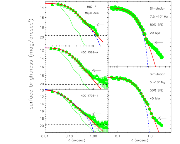
Figure 2.: Surface brightness profiles for three young clusters (left - M82-F, NGC 1569-A, and NGC 1705-1) and two $N$-body simulations which include the rapid removal of gas which was left over from a non-100% star-formation efficiency (right). The solid (red) and dashed (blue) lines are the best fitting EFF (Elson et al. 1987) and King (King 1962) profiles respectively. Note the excess of light at large radii with respect to the best fitting EFF profile in both the observations and models. This excess light is due to an unbound expanding halo of stars caused by the rapid ejection of the remaining gas after the cluster forms. Hence, excess light at large radii strongly implies that these clusters are not in dynamical equilibrium. For details of the modeling and observations see Bastian & Goodwin (2006) and Goodwin & Bastian (2006).

2.2. Interpretation of the properties of young clusters

Even if a cluster survives the gas removal phase, this phase can significantly effect the observed properties of the cluster. Hence, deducing the initial properties of a cluster from its current state is not trivial. Kroupa & Boily (2002) have noted the strong effect of residual gas removal on inferring the initial stellar mass of a cluster, while Goodwin & Bastian (2006) have refined the mass loss estimates and shown that measurements of the current radii of young clusters may not reflect the initial nor the final value. Additionally, Goodwin & Bastian (2006) show that this effect can mimic stellar IMF variations in young clusters.

3. Population Studies of Cluster Disruption

The clusters that have survived the gas removal phase are subject to disruption Phases II and III (§ 1.1.) as well as tidal effects. Disruption due to these effects can be studied on individual clusters, of which the recent observations of the dissolving globular clusters Palomar 5 (Odenkirchen et al. 2001) are probably the most spectacular example. However, much can be learned by approaching this problem from a cluster population point of view.

3.1. The Lamers disruption law

Suppose that clusters are formed continuously with a constant cluster formation rate (a constraint which we can relax later). Also, we will assume that we know the cluster initial mass function (here taken to be a power law of the form $\mbox{${N_{\rm cl}}$}\mbox{${\mbox{d}}$}\mbox{${M_{\rm cl}}$}\propto\mbox{${M_{\rm cl}}$}^{-\alpha}\mbox{${\mbox{d}}$}\mbox{${M_{\rm cl}}$}$ with ${\alpha}=2$ (e.g. Zhang & Fall 1999; de Grijs et al. 2003) and that clusters can be detected down to a known magnitude limit. Finally, we will assume that the disruption time of a cluster depends on the cluster mass, such that more massive clusters survive longer (on average) than lower mass clusters. For this final assumption we will adopt a function of the form:

$$\mbox{$t_{\rm dis}$}=t_{4}(\mbox{${M_{\rm cl}}$}/10^{4}M_{\odot})^{\gamma},$$ (1)

where $t_{4}$ is the disruption time of a $10^{4}\,M_{\odot}$ cluster and $0<\gamma<1$ (Boutloukos & Lamers 2003). The beauty of this formulation is that it only has two variables, $t_{4}$ and $\gamma$, and as we will see, provides extremely good fits to observations.

3.2. Application to various cluster populations

The formulation provided above, when combined with the given assumptions, allows for the parameters $t_{4}$ and $\gamma$ to be found from age and mass distributions of clusters. The first survey using this technique was carried out by Boutloukos & Lamers (2003) on cluster populations in M51, M33, the SMC, and the solar neighbourhood. They made a sudden disruption assumption, meaning that the cluster is in the sample with its initial mass until $t_{\rm dis}$, when it is disrupted. The somewhat surprising result from this study was that, while $\gamma$ had more or less the same value in all environments studied ($\langle\gamma\rangle=0.62\pm 0.06$), $t_{4}$ varied by over two orders of magnitude, with values of $\sim 80$ Myr in the central regions of M51 to $\sim 8$ Gyr in the SMC.

The simple sudden disruption assumption was improved in a more recent model by Lamers et al. (2005a), where a gradual loss of cluster mass was implemented. They assumed that the cluster mass decreases exponentially with a time-scale that decreases as the cluster mass decreases. This is done by saying that the mass loss per unit time ($\dot{M}$) relates to $t_{\rm dis}$ as:

$$\mbox{$\dot{M}$}=\mbox{${M_{\rm cl}}$}/\mbox{$t_{\rm dis}$}\propto\mbox{${M_{\rm cl}}$}^{1-\gamma},$$ (2)

with $t_{\rm dis}$ from Eq. 1. This very simple analytical description for cluster mass loss shows remarkably good agreement when compared to the mass loss following from the detailed $N$-body simulations of Baumgardt & Makino (2003). In Fig. 3 we show a direct comparison of $\dot{M}$ from the $N$-body simulations of clusters with different density profiles and on different orbits (left) and the above mentioned analytical model of Lamers et al. (2005a) (right).

In both graphs the time is normalised to $t_{\rm dis}$ and only the mass loss due to stars escaping the cluster is shown, i.e. mass loss due to stellar evolution (SEV) is not shown. In addition, there is a coupling between the two types of mass loss: if stars loose mass, the cluster will expand and more stars are pushed over the tidal boundary. The simulations of Baumgardt & Makino (2003) considered SEV, therefore, their $\dot{M}$ results shown in Fig. 3 do include tidal $\dot{M}$ induced by SEV. For this reason we can simply add the mass loss due to SEV, taken from an SSP model, to Eq. 2.

Figure 3.: Comparison between the mass loss following from the $N$-body simulations of clusters with different number of stars, different concentration and on different orbits (left). The mass loss due to stellar evolution is not shown. In the right panel the analytical model of Lamers et al. (2005a) is shown.

In a series of follow-up works, it has been shown that the similarity of the value of $\gamma$ in various environments strongly implies a uniformity in the cluster disruption process, while the varying values of $t_{4}$ is due to the different tidal field strengths (and gas contents) of the galaxies studied. Galaxies with strong tidal fields, as, for example, derived from their rotation curves, having shorter disruption times (Lamers et al. 2005b). Comparison with results of realistic $N$-body models performed by Baumgardt & Makino (2003) have placed this empirical disruption law on a solid physical footing (Lamers et al. 2005a). Lamers et al. (2005a) have also derived a formula for the predicted mass and age distributions of cluster samples that includes both stellar evolution and disruption for any star formation history.

Gieles et al. (2005) inserted the Lamers disruption law into a cluster population synthesis model. This method has two distinct advantages over the earlier formulations. The first is that it removes the requirement of a constant cluster formation rate, and second, it uses the age and mass distributions together to find $\gamma$ and $t_{4}$. The case of M51 is shown in Fig. 4. One first begins by constructing an observed number density grid in age-mass space (upper-left panel where the shading corresponds to the logarithm of the number of clusters found within that cell). Then one generates a large number of models with different values of $t_{4}$, $\gamma$, (time dependent) cluster formation rates, etc. and compares these models with the observed grid. The resultant $\chi^{2}_{\nu}$ diagram is shown in the bottom panel of Fig. 4. The best fit model is shown in the top right panel of Fig. 4.

This cluster population synthesis (CPS) technique, also used in a similar way by Dolphin & Kennicutt (2002) to derive the properties of the cluster population in the galaxy NGC 3627, holds great promise in disentangling the myriad of effects present in cluster populations. In principle, the dependences of cluster size, galactocentric radius, star-formation efficiency dependent infant mortality rates, or alternative cluster disruption models can be taken into account by this technique. For this technique to be fully exploited one needs large samples of cluster populations with known ages and masses. Datasets suitable for these kind of studies are beginning to be collected and released. Several face-on spiral galaxies have been imaged in multiple filters with the high resolution/wide field HST/ACS camera (e.g Barmby et al. 2006 for M101 and Gieles et al. 2006b for M51).

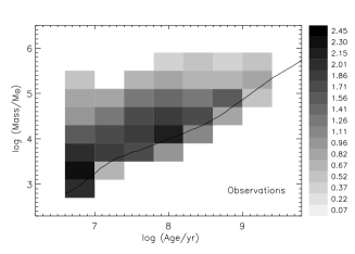
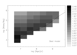
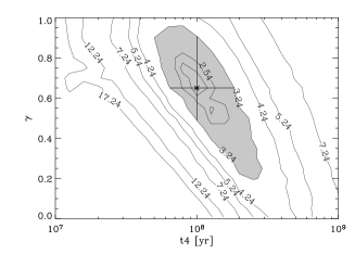
Figure 4.: Top left panel: The observed age-mass diagram of clusters in M51. The shading represents the logarithm of the number of clusters found within the corresponding box in age-mass space. The solid line represents the detection limit of the sample. Top right panel: The best fitting cluster population synthesis model which includes the detection limit of the observations and has fit on $\gamma$ and $t_{4}$. Bottom: The $\chi^{2}_{\nu}$ diagram in $\gamma$-$t_{4}$ space. The best fitting model is marked with an ’x’, while the accepted fits ($\chi^{2}_{\nu}<\chi^{2}_{\nu,{\rm best}}+1$) are shaded. Reproduced from Gieles et al. (2005).

3.3. Possible objections

It is worth noting possible objections to the Lamers disruption law. The first comes from Fall et al. (2005) who find that in the Antennae galaxies the number of clusters decreases in time ($\tau$) as $\mbox{${\mbox{d}}$}N/\mbox{${\mbox{d}}$}\tau\propto\tau^{-1}$, independent of cluster mass. This may be explained if the disruption timescale $t_{4}$ due to tidal field effects (e.g. Phase II & III) is greater than or similar to the maximum age in the sample. The cluster disruption due to tidal effects would not yet be present in the Fall et al. (2005) sample, instead the decrease in cluster numbers would be the result of infant mortality and the fading of clusters. Studies of infant mortality in M51 also suggest that the effect is mass independent (Bastian et al. 2005). In fact, if infant mortality was not (mostly) independent of cluster mass we would expect the embedded cluster mass function to be significantly different from the optically selected cluster mass function.

In Fig. 5 we show the dependence of the mass function slope of a multiple age cluster population on the ratio of the $t_{4}$ and the maximum age of the cluster in the sample ($t_{\rm max}$). Clusters were created continuously over 1 Gyr with an initial mass function of a power-law with index $-2$. The Lamers disruption law was applied in the same way as in Gieles et al. (2005). The important thing to take away from this figure is that as $t_{\rm dis}$ approaches and exceeds $t_{\rm max}$ the mass function is less affected by disruption and so it retains its initial form, i.e. the right panel in Fig. 5 probably applies to the Fall et al. (2005) sample.

Figure 5.: Representation of how the slope of the mass function changes as a function of the ratio between the disruption time ($t_{\rm dis}$) and the age of the oldest cluster in the sample (in this case assuming a constant cluster formation rate). Note that if $t_{\rm dis}$ approaches or exceeds $t_{\rm max}$ the slope of the mass function approaches the initial mass function value (i.e. $-2$).

A second observation seemingly contradicting the Lamers disruption law is that of Chandar et al. (2006) who find an intermediate age ($\sim 4-7$ Gyr) globular cluster in M33. In M33, Lamers et al. (2005b) find a $t_{4}$ value of $\sim 600$ Myr, implying a disruption time of $\sim 2.5$ Gyr for a $10^{5}~{}M_{\odot}$ cluster. However, as the authors note, the value of $t_{4}$ derived by Lamers et al. (2005b) was presumably of the thin disk of the galaxy, and if the intermediate-age cluster is part of the thick-disk or halo of the galaxy then the expected value of $t_{4}$ would be significantly larger than that quoted. Additionally, it should also be noted that the mass derived by Chandar et al. (2006) is the present mass of the cluster. The cluster presumably started with a much higher mass and disruptive effects have brought this cluster into its current state. If the present mass of the cluster is $1\times 10^{5}$ ${\rm M}_{\odot}$, then its initial mass (after infant weight loss) would have been $5\times 10^{5}$ ${\rm M}_{\odot}$(assuming an age of 5 Gyr), using the value of $t_{4}$ for M33 given by Lamers et al. (2005b).

4. External Disruption Effects: GMCs and Spiral Arms

4.1. The disruption time due to external perturbations

Figure 6.: Comparison between the observed (filled circles) and predicted (solid line; from the $N$-body models of Baumgardt & Makino 2003) disruption time of a $10^{4}~{}M_{\odot}$ cluster, $t_{4}$, as a function of the mean density $\rho_{\rm amb}$ in $M_{\odot}$pc^-3 of the host galaxy. Reproduced from Lamers et al. (2005b).

As more and more galaxies (and environments) have their characteristic disruption timescales measured, it is useful to compare the results to $N$-body models in order to check for consistency between the two. This was done in Lamers et al. (2005b) who compared the $t_{4}$ values derived for the SMC, M33, M51 and the solar neighbourhood to the $N$-body models of Baumgardt & Makino (2003) and Portegies Zwart et al. (1998, 2002) which sample a large range in the ambient densities of the host galaxies. Their results, shown in Fig. 6, are intriguing. While the predicted and observed disruption time of the SMC are in excellent agreement, the disruption times of the Galaxy, M33 and M51 are observed to be much shorter than predicted by $N$-body models. This result is particularly surprising given the fact that the mass loss predictions of a single cluster are in excellent agreement between the Lamers empirical description and that given by $N$-body models (Lamers et al. 2005a and Fig. 3).

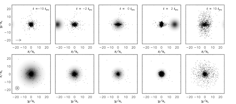
Figure 7.: Snapshots of a star cluster undergoing a head-on encounter with a GMC of M_n = $10^{4}~{}M_{\odot}$ with $V_{\rm max}=20\sigma_{\rm rms}$. Top: The motion of the GMC is along the x-axis and the line of sight is perpendicular. Bottom: The motion of the GMC is into the page and the line of sight is along the GMC trajectory. The arrows in the left-hand lower corner of the left-hand panels are parallel to the direction of motion of the GMC. The GMC is shown with grey shades based on the surface density of a GMC with a_n = 5.8a_c. The time with respect to the moment of encounter is indicated in each panel of the top row. See Gieles et al. (2006c) for a description of the methods and parameters used.

Thus, we are left to ask, what physical effects are not included in the $N$-body models that may be responsible for disrupting clusters? The $N$-body models used in the comparison were carried out in a smooth logarithmic potential which does not realistically represent the thin disk components of disk galaxies. Gieles et al. (2006a, c) have attempted to add encounters with giant molecular clouds (GMCs) and spiral arm passages to the $N$-body models. In Fig. 7 we show an example of a cluster-GMC encounter (from Gieles et al. 2006c). The parameters of this run are for typical open clusters and GMCs in the solar neighbourhood. The top panels show an edge-on view for five different time steps, while the bottom panels show a view along the trajectory of the GMC.

Encounters with GMCs present the most important external perturbation which cause mass loss of star in clusters. Gieles et al. (2006c) find that $t_{\rm dis}$ due to encounters with GMCs scales as

$$\mbox{$t_{\rm dis}$}=2.0\,S\left(\frac{\mbox{${M_{\rm cl}}$}}{10^{4}\,\mbox{${\rm M}_{\odot}$}}\right)\left(\frac{3.75\,{\rm pc}}{\mbox{$r_{\rm h}$}}\right)^{3}{\mbox{Gyr}},$$ (3)

where $S\equiv 1$ for the solar neighbourhood and $S$ scales with the surface density of individual GMCs ($\Sigma_{\rm n}$) and the global GMC density ($\rho_{\rm n}$) as $S\propto(\mbox{$\Sigma_{\rm n}$}\mbox{$\rho_{\rm n}$})^{-1}$. The scaling of $S$ with $\rho_{\rm n}$ implies that it does not matter if the molecular gas is distributed over a large number of low mass clouds or a small number of massive (giant) clouds. This makes it easy to estimate $t_{\rm dis}$ from the observed molecular gas density. Indeed, for M51, where the molecular gas density is about an order of magnitude higher than in the solar neighbourhood, a $t_{\rm dis}$ from Eq. 3 of 150 Myr is predicted. This corresponds well with the value derived from observations of $t_{4}=100-200$ Myr (Gieles et al. 2005).

Note that Eq. 3 implies a scaling of $t_{\rm dis}$ with the cluster density ($\rho_{\rm cl}$). This seems different than the dependence with ${M_{\rm cl}}$ discussed before. However, there is only a very shallow relation observed between cluster half-mass radius ($r_{\rm h}$) and ${M_{\rm cl}}$, of the form $\mbox{$r_{\rm h}$}\propto\mbox{${M_{\rm cl}}$}^{0.1}$ (Larsen 2004). With this relation, and Eq. 3, it follows that for external perturbations $\mbox{$t_{\rm dis}$}\propto\mbox{${M_{\rm cl}}$}^{0.7}$, i.e. very close to the index of $\gamma\simeq 0.6$ found from observations discussed in § 3.2.. This suggests that the disruptive effect of the tidal field and additional external perturbations can be added linearly, resulting in a $t_{\rm dis}$ that depends on ${M_{\rm cl}}$ as $\mbox{$t_{\rm dis}$}\propto\mbox{${M_{\rm cl}}$}^{0.6}$. This can explain the large variation found in the $t_{4}$ value derived from observations and the almost constant $\gamma=0.6$ (Boutloukos & Lamers 2003). In § 5. we discuss some of the pitfalls of these results.

4.2. Application to the open clusters in the Galaxy

As seen in the proceeding sections, the observed disruption time of star clusters in the solar neighbourhood is a factor of $\sim 5$ shorter than predicted by $N$-body models. The inclusion of spiral arm passages and GMC encounters into $N$-body models is a promising way to bring the predictions into agreement with the observations. This was recently done by Lamers & Gieles (2006) who found excellent agreement after the inclusion GMC encounters and spiral arm passages. They assume that the different mass loss effects (stellar evolution, tidal field and external perturbations) can be added linearly. Using the mass-radius relation of § 4.1. and the results from Gieles et al. (2006a) and Gieles et al. (2006c) they analytically model the mass loss due to different effects analytically. This is illustrated in the left panel of Fig. 8 (from Lamers & Gieles 2006). Based on this mass loss description, the age distribution of open clusters in the solar neighbourhood can be predicted (instead of fitted, as was done hitherto). The results are shown in the right panel of Fig. 8.

Figure 8.: Left: The mass evolution of a $10^{4}\mbox{${\rm M}_{\odot}$}$ cluster due to various disruptive effects. Right: Comparison between the observed age distribution of open clusters (from Kharchenko et al. 2005) and the predictions from Lamers & Gieles (2006) for three different maximum masses.

5. Discussion

We showed in §§ 3.&4. that the simple Lamers disruption law can successfully explain the age and mass distribution of young star clusters populations. Here we will discuss other observations lending support to the Lamers law and some of the standing problems and uncertainties of this scenario which need further attention.

5.1. Independent checks on the disruption law

It is reassuring to see that different datasets of various cluster populations all come to similar conclusions regarding the disruption of clusters.

de Grijs & Anders (2006) use a variety of studies to look at the cluster population of the LMC. They also find a lack of old clusters (with respect to what would be expected from a continuous cluster formation rate) and derive $\gamma=0.56$, again in agreement with other galaxies studied by Boutloukos & Lamers (2003) and Lamers et al. (2005a). Note that a lower value of $\gamma$ is expected to be observed when the typical $t_{\rm dis}$ is of the same order as the oldest clusters in the sample (Fig. 5), as is the case in LMC.

Outside the local group, the strongly interacting galaxy NGC 6745 has been studied by de Grijs et al. (2003) who found evidence for mass dependent disruption, with $\gamma=0.54$. The rich cluster system of the intermediate-age merger remnant NGC 1316 shows a clear bimodal colour distribution, with the red component presumably being formed during the merger. Goudfrooij et al. (2004) showed, using deep HST-ACS images that if one breaks the red component into ‘inner’ and ‘outer’ regions (with respect to the galactic centre), that the outer region is a continuous power-law while the inner region shows a power-law behavior at the high luminosity end and a flattening at the low luminosity end. The authors interpret this as evidence for mass-dependent cluster disruption, although no attempt was made to find the characteristic disruption timescale or the value of $\gamma$.

One standing problem with the Lamers disruption law, also present in other studies on disruption, is whether or not an initial power-law cluster initial mass function (CIMF) can be transformed into a log-normal distribution, which is observed for old globular cluster populations. The Lamers law can create such a turnover, however the precise value of the turnover mass should be dependent on the ambient density (Lamers et al. 2005b), meaning that cluster disruption should be more efficient in the inner regions of a galaxy than in the outer regions. Thus, without fine tuning the models (e.g. having the same disruption time at all radii due to large radially dependent velocity anisotropies) one would expect a radially dependent turnover peak in the globular cluster mass function, which is not observed. For a more detailed description of this problem, see the review by Larsen in these proceedings. Additionally, as noted by Waters et al. (2006) the Lamers disruption over-predicts the number of low-mass clusters when applied to old globular cluster populations.

5.2. Caveats in the theoretical underpinning

In § 4.1. we showed that the scaling of $t_{\rm dis}$ with ${M_{\rm cl}}$ is a power-law with exponent $\gamma\simeq 0.6$. This scaling is similar for two-body evaporation in a tidal field with external perturbations, such as shocks by GMCs and spiral arms, and agrees well with the observations. However, there are still some caveats in the theory explaining this, mostly coming from questions regarding the initial conditions of the simulations.

1. The first caveat stems from the relation between initial mass and radius of the clusters used in the simulations. If we parameterize this relation as $r_{\rm h}$ $\propto$ ${M_{\rm cl}}$^λ, then Baumgardt & Makino (2003) use $\lambda=1/3$, implying that their clusters fill their tidal radius. However, observations imply that $\lambda=0-0.1$ (with a large scatter) (Larsen 2004; Bastian et al. 2005), implying that $r_{\rm h}$ is mostly independent of mass. This shallow relation implies that massive clusters are not filling their tidal radius, which would change the dependence of $t_{\rm dis}$ with ${M_{\rm cl}}$ (Tanikawa & Fukushige 2005).

2. In the derivation of $\gamma$ for external shocks (§ 4.1.), only clusters in isolation were considered. How would the presence of a tidal field affect this result?

3. How does the relation for $t_{\rm dis}$ change if there exists a relation between the concentration parameter and mass of a cluster (i.e. as seen in the Galactic GCs reported by Larsen in these proceedings)?

4. Could an initial mass-radius relation with $\lambda=1/3$ be erased during the gas removal phase?

5. What is the effect of the initial mass/luminosity profile used in the simulations and how does it evolve? e.g. are clusters born with EFF profiles which are converted into King profiles? Does the cluster concentration alter its mass loss evolution?

6. How do the external perturbations and the galactic tidal field cooperate? Can the mass loss due to both effects simply be added linearly?

Acknowledgments.

Both NB and MG are grateful to Henny for all of his guidance, ideas and help.

References

- Barmby et al. (2006) Barmby, P., Kuntz, K. D., Huchra, J. P., & Brodie, J. P. 2006, AJ, 132, 883
- Bastian & Goodwin (2006) Bastian, N. & Goodwin, S.P. 2006, MNRAS, 369, L9
- Bastian et al. (2005) Bastian, N., Gieles, M., Lamers, H.J.G.L.M., Scheepmaker, R. A., & de Grijs, R. 2005, A&A 431, 905
- Baumgardt & Makino (2003) Baumgardt, H., & Makino, J. 2003, MNRAS, 340, 227
- Baumgardt (2006) Baumgardt, H. 2006: Globular Clusters: Guides to Galaxies (astro-ph/0605125)
- Boily & Kroupa (2003a) Boily, C.M. & Kroupa, P. 2003a, MNRAS, 338, 665
- Boily & Kroupa (2003b) Boily, C.M. & Kroupa, P. 2003b, MNRAS, 338, 673
- Boutloukos & Lamers (2003) Boutloukos, S.G. & Lamers, H.J.G.L.M. 2003, MNRAS, 338, 717
- Chandar et al. (2005) Chandar, R., Leitherer, C., Tremonti, C.A., Calzetti, D., Aloisi, A., Meurer, G.R., & de Mello, D. 2005, ApJ, 628, 210
- Chandar et al. (2006) Chandar, R., Puzia, T.H., Sarajedini, A., Goudfrooij, P. 2006, ApJL, in press (astro-ph/0606419)
- de Grijs et al. (2003) de Grijs, R., Anders, P., Bastian, N., Lynds, R., Lamers, H.J.G.L.M., O’Neil, E.J. 2003, MNRAS, 343, 1285
- de Grijs & Anders (2006) de Grijs, R., & Anders, P. 2006, MNRAS, 366, 295
- Dolphin & Kennicutt (2002) Dolphin, A.E., & Kennicutt, R.C. 2002, AJ, 124, 158
- Elson et al. (1987) Elson, R.A.W., Fall, M.S., & Freeman, K.C. 1987, ApJ 323, 54 (EFF)
- Fall & Zhang (2001) Fall, S. M. & Zhang, Q. 2001, ApJ, 561, 751
- Fall et al. (2005) Fall, S.M., Chandar, R. & Whitmore, B.C. 2005, ApJ, 631, L133
- Gascoigne (1966) Gascoigne, S. C. B. 1966, MNRAS, 134, 59
- Gieles et al. (2005) Gieles, M., Bastian, N., Lamers, H.J.G.L.M., & Mout, J.N. 2005, A&A, 441, 949
- Gieles et al. (2006a) Gieles, M., Athanassoula E., Portegies Zwart S. F., 2006b, MNRAS, submitted
- Gieles et al. (2006b) Gieles, M., Larsen, S. S., Scheepmaker, R. A., et al. 2006b, A&A, 446, L9
- Gieles et al. (2006c) Gieles, M., Portegies Zwart, S.F., Baumgardt, H. Athanassoula, E., Lamers, H.J.G.L.M., Sipior, M., Leenaarts, J. 2006c, MNRAS, 371, 793
- Goudfrooij et al. (2004) Goudfrooij, P., Gilmore, D., Whitmore, B.C., & Schweizer, F. 2004, ApJ, 613, L121
- Goodwin (1997a) Goodwin, S.P. 1997a, MNRAS, 284, 785
- Goodwin (1997b) Goodwin, S.P. 1997b, MNRAS, 286, 669
- Goodwin & Bastian (2006) Goodwn, S.P. & Bastian, N. 2006, MNRAS, in press (astro-ph/0609477)
- Hodge (1987) Hodge, P. 1987, PASP, 99, 724
- Kharchenko et al. (2005) Kharchenko, N. V., Piskunov, A. E., Röser, S., Schilbach, E., & Scholz, R.-D. 2005, A&A, 438, 1163
- King (1962) King, I. 1962, AJ 67, 471
- Kroupa & Boily (2002) Kroupa, P. & Boily, C.M. 2002, MNRAS, 336, 1188
- Lada & Lada (2003) Lada, C.J. & Lada, E.A. 2003, ARA&A, 41, 57
- Lamers et al. (2005a) Lamers, H.J.G.L.M., Gieles, M., Bastian, N., Baumgardt, H., & Kharchenko, N.V. 2005a, A&A, 117, 129
- Lamers et al. (2005b) Lamers, H.J.G.L.M., Gieles, M., & Protegies Zwart, S.F. 2005b, A&A, 429, 173
- Lamers & Gieles (2006) Lamers, H.J.G.L.M. & Gieles, M. 2006, A&A, 455, L17
- Larsen (2004) Larsen, S. S. 2004, A&A, 416, 537
- Odenkirchen et al. (2001) Odenkirchen, M., et al. 2001, ApJ, 548, L165
- Oort (1958) Oort, J. H. 1958, Ricerche Astronomiche, 5, 507
- Portegies Zwart et al. (1998) Portegies Zwart, S.F., Hut, P., & Makino, J. 1998, A&A, 337, 363
- Portegies Zwart et al. (2002) Portegies Zwart, S.F., Makino, J., McMillan, S.L.W., & Hut, P. 2002, ApJ, 565, 265
- Schweizer (2006) Schweizer, F. 2006: Globular Clusters: Guides to Galaxies (astro-ph/0606036)
- Spitzer (1987) Spitzer, L. 1987, Dynamical evolution of globular clusters (Princeton, NJ, Princeton University Press, 1987, 191 p.)
- Tanikawa & Fukushige (2005) Tanikawa, A., & Fukushige, T. 2005, PASJ, 57, 155
- Tremonti et al. (2001) Tremonti, C.A., Calzetti, D., Leitherer, C., & Heckman, T.M. 2001, ApJ, 555, 322
- Tutukov (1978) Tutukov, A.V. 1978, A&A, 70, 57
- Vesperini (1998) Vesperini, E. 1998, MNRAS, 299, 1019
- Vesperini & Zepf (2003) Vesperini, E. & Zepf, S. E. 2003, ApJ, 587, L97
- Waters et al. (2006) Waters, C.Z., Zepf, S.E., Lauer, T.R, Baltz, E.A., & Silk, J. 2006, ApJ, in press (astro-ph/0607238)
- Wielen (1971) Wielen, R. 1971, A&A, 13, 309
- Whitmore et al. (1999) Whitmore, B.C. Zhang, Q., Leitherer, C., et al. 1999b, AJ, 118, 1551
- Whitmore (2003) Whitmore, B. C. 2003, in A Decade of HST Science, eds. Mario Livio, Keith Noll & Massimo Stiavelli, (Cambridge: Cambridge University Press), 153. (widely referenced as Whitmore 2000, astro-ph/0012546)
- Zhang & Fall (1999) Zhang, Q., & Fall, S. M. 1999, ApJ, 527, L81