Astrometry in Wide-field Surveys

Abstract

We present a robust and fast algorithm for performing astrometry and source cross-identification on two dimensional point lists, such as between a catalogue and an astronomical image, or between two images. The method is based on minimal assumptions: the lists can be rotated, magnified and inverted with respect to each other in an arbitrary way. The algorithm is tailored to work efficiently on wide fields with large number of sources and significant non-linear distortions, as long as the distortions can be approximated with linear transformations locally, over the scale-length of the average distance between the points. The procedure is based on symmetric point matching in a newly defined continuous triangle space that consists of triangles generated by an extended Delaunay triangulation. Our software implementation performed at the 99.995% success rate on $\sim 260,000$ frames taken by the HATNet project.

1. Introduction

Cross-matching two two-dimensional points lists is a crucial step in astrometry and source identification. The tasks involves finding the appropriate geometrical transformation that transforms one list into the reference frame of the other, followed by finding the best matching point-pairs. One of the lists usually contains the pixel coordinates of sources in an astronomical image (e.g. point-like sources, such as stars), while the other list can be either a reference catalog with celestial coordinates, or it can also consist of pixel coordinates that originate from a different source of observation (another image). Throughout this paper we denote the reference (list) as $\mathcal{R}$, the image (list) as $\mathcal{I}$, and the function that transforms the reference to the image as $\mathcal{F}_{R\rightarrow I}$.

The difficulty of the problem is that in order to find matching pairs, one needs to know the transformation, and vica versa: to derive the transformation, one needs point-pairs. Furthermore, the lists may not fully overlap in space, and may have only a small fraction of sources in common.

By making simple assumptions on the properties of $\mathcal{F}_{R\rightarrow I}$, however, the problem can be tackled. A very specific case is when there is only a simple translation between the lists, and one can use cross-correlation techniques (see Phillips & Davis, 1995) to find the transformation. We note, that the a method proposed by Thiebaut & Boër (2001) uses the whole image information to derive a transformation (translation and magnification).

A more general assumption, typical to astronomical applications, is a that $\mathcal{F}_{R\rightarrow I}$ is a similarity transformation (rotation, magnification, inversion, without shear), i.e. $\mathcal{F}_{R\rightarrow I}=\lambda\mathbf{A}\underline{r}+\underline{b}$, where $\mathbf{A}$ is a (non-zero) scalar $\lambda$ times the orthogonal matrix, $\underline{b}$ is an arbitrary translation, and $\underline{r}$ is the spatial vector of points. Exploiting that geometrical patterns remain similar after the transformation, more general algorithms have been developed that are based on pattern matching (Groth, 1986; Valdes et al., 1995). The idea is that the initial transformation is found by the aid of a specific set of patterns that are generated from a subset of the points on both $\mathcal{R}$ and $\mathcal{I}$. For example, the subset can be that of the brightest sources, and the patterns can be triangles. With the knowledge of this initial transformation, more points can be cross-matched, and the transformation between the lists can be iteratively refined. Some of these methods are implemented as an iraf task in immatch (Phillips & Davis, 1995).

The above pattern matching methods perform well as long as the dominant term in the transformation is linear, such as for astrometry of narrow field-of-view (FOV) images, and as long as the number of sources is small (because of the large number of patterns that can be generated – see later). In the past decade of astronomy, with the development of large format CCD cameras or mosaic imagers, many wide-field surveys appeared, such as those looking for transient events (e.g. ROTSE — Akerlof et al. 2000), transiting planets (e.g. Kelt – Pepper, Gould, & Depoy 2004, TrES – Alonso et al. 2004, HATNet – Bakos 2002, 2004, see Charbonneau 2006 for further references), or all-sky variability (e.g. ASAS – Pojmanski 1997). There are non-negligible, higher order distortion terms in the astrometric solution that are due to, for instance, the projection of celestial to pixel coordinates and the properties of the fast focal ratio optical systems. Furthermore, these images may contain $\sim 10^{5}$ sources, and pattern matching is non-trivial.

These surveys necessitated a further generalization of the algorithm, which we present in this paper. To be more specific, we were motivated by the astrometric requirements of the Hungarian-made Automated Telescope Network (HATNet). Each HAT telescope of the Network consists of a $f=200\mathrm{mm}$, $d=f/1.8$ telephoto lens and a $\rm 2K\times\rm 2K$ CCD yielding an $8\arcdeg\times 8\arcdeg$ FOV. In our experience, we need at least 4th order polynomial functions of the pixel coordinates in order to properly describe the distortion of the lens. With a typical exposure time of 5 minutes in I-band, in a moderately dense field ($b\approx 15^{\circ}$) there are 30000 stars brighter than I=13 for which better than 10% photometry can be achieved. If we consider all 3-$\sigma$ detections, we have to deal with the identification of $\sim$100,000 sources.

The algorithm presented in this paper is based on, and is a generalization of the above pattern matching algorithms. It is very fast, and works robustly for wide-field imaging with minimal assumptions. Namely, we assume that: i) the distortions are non-negligible, but small compared to the linear term, ii) there exists a smooth transformation between the reference and image points, iii) the point lists have a considerable number of sources in common, and iv) the transformation is locally invertible. The paper is presented as follows. First we describe symmetrical point matching in § 2 before we go on to the discussion of finding the transformation (§ 3). The software implementation and its performance on a large and inhomogeneous dataset is demonstrated in § 4. Finally, we draw conclusions in § 5.

2. Symmetric point matching

First, let us assume that $\mathcal{F}_{R\rightarrow I}$ is known. To find point-pairs between $\mathcal{R}$ and $\mathcal{I}$  one should first transform the reference points to the reference frame of the image: $\mathcal{R^{\prime}}=\mathcal{F}_{R\rightarrow I}(\mathcal{R})$. Now it is possible to perform a simple symmetric point matching between $\mathcal{R^{\prime}}$ and $\mathcal{I}$. One point ($R_{1}\in\mathcal{R^{\prime}}$) from the first and one point ($I_{1}\in\mathcal{I}$) from the second set are treated as a pair if the closest point to $R_{1}$ is $I_{1}$ and the closest point to $I_{1}$ is $R_{1}$. This requirement is symmetric by definition and excludes such cases when e.g. the closest point to $R_{1}$ is $I_{1}$, but there exists an $R_{2}$ that is even closer to $I_{1}$, etc.

In one dimension, finding the point of a given list nearest to a specific point ($x$) can be implemented as a binary search. Let us assume that the point list with $N$ points is ordered in ascending order. This has to be done only once, at the beginning, and using the quicksort algorithm, for example, the required time scales on average as $\mathcal{O}(N\log N)$. Then $x$ is compared to the median of the list: if it is less than the median, the search can be continued recursively in the first $N/2$ points, if it is greater than the median, the second $N/2$ half is used. At the end only one comparison is needed to find out whether $x$ is closer to its left or right neighbor, so in total $1+\log_{2}(N)$ comparisons are needed, which is an $\mathcal{O}(\log N)$ function of $N$. Thus, the total time including the initial sorting also goes as $\mathcal{O}(N\log N)$.

As regards a two dimensional list, let us assume again, that the points are ordered in ascending order by their $x$ coordinates (initial sorting $\sim\mathcal{O}(N\log N)$), and they are spread uniformly in a square of unit area. Finding the nearest point in $x$ coordinate also requires $\mathcal{O}(\log N)$ comparisons, however, the point found presumably will not be the nearest in Euclidean distance. The expectation value of the distance between two points is $1/\sqrt{N}$, and thus we have to compare points within a strip with this width and unity height, meaning $\mathcal{O}(\sqrt{N})$ comparisons. Therefore, the total time required by a symmetric point matching between two catalogs in two dimensions requires $\mathcal{O}(N^{3/2}\log N)$ time.

We note that finding the closest point within a given set of points is also known as nearest neighbor problem (for a summary see Gionis, 2002, and references therein). It is possible to reduce the computation time in 2 dimensions to $\mathcal{O}(N\log N)$ by the aid of Voronoi diagrams and Voronoi cells, but we have not implemented such an algorithm in our matching codes.

3. Finding the transformation

Let us go back to finding the transformation between $\mathcal{R}$ and $\mathcal{I}$. The first, and most crucial step of the algorithm is to find an initial “guess” $\mathcal{F}^{(1)}_{R\rightarrow I}$ for the transformation based on a variant of triangle matching. Using $\mathcal{F}^{(1)}_{R\rightarrow I}$, $\mathcal{R}$ is transformed to $\mathcal{I}$, symmetric point-matching is done, and the paired coordinates are used to further refine the transformation (leading to $\mathcal{F}^{(i)}_{R\rightarrow I}$ in iteration $i$), and increase the number of matched points iteratively. A major part of this paper is devoted to finding the initial transformation.

3.1. Triangle matching

It was proposed earlier by Groth (1986) and Stetson (1989), and recently by others (see Valdes et al., 1995) to use triangle matching for the initial “guess” of the transformation. The total number of triangles that can be formed using $N$ points is $N(N-1)(N-2)/6$, an $\mathcal{O}(N^{3})$ function of $N$. As this can be an overwhelming number, one can resort to using a subset of the points for the vertices of the triangles to be generated. One can also limit the parameters of the triangles, such as exclude elongated or large (small) triangles.

As triangles are uniquely defined by three parameters, for example the length of the three sides, these parameters (or their appropriate combinations) naturally span a 3-dimensional triangle space. Because our assumption is that $\mathcal{F}_{R\rightarrow I}$ is dominated by the linear term, to first order approximation there is a single scalar magnification between $\mathcal{R}$ and $\mathcal{I}$ (besides the rotation, chirality and translation). It is possible to reduce the triangle space to a normalized, two-dimensional triangle space ($(T_{x},T_{y})\in T$), whereby the original size information is lost. Similar triangles (with or without taking into account a possible flip) can be represented by the same points in this space, alleviating triangle matching between $\mathcal{R}$ and $\mathcal{I}$.

3.1.1 Triangle spaces

There are multiple ways of deriving normalized triangle spaces. One can define a “mixed” normalized triangle space $T^{\text{(mix)}}$, where the coordinates are insensitive to inversion between the original coordinate lists, i.e. all similar triangles are represented by the same point irrespective of their chirality (Valdes et al., 1995):

$$T^{\text{(mix)}}_{x} = p/a,$$ (1)

$$T^{\text{(mix)}}_{y} = q/a,$$ (2)

where $a$, $p$ and $q$ are the sides of the triangle in descending order. Triangles in this space are shown on the left panel of Fig. 1. Coordinates in the mixed triangle space are continuous functions of the sides (and therefore of the spatial coordinates of the vertices of the original triangle) but the orientation information is lost. Because we assumed that $\mathcal{F}_{R\rightarrow I}$ is smooth and bijective, no local inversions and flips can occur. In other words, $\mathcal{R}$ and $\mathcal{I}$ are either flipped or not with respect to each other, but chirality does not have a spatial dependence, and there are no “local spots” that are mirrored. Therefore, using mixed triangle space coordinates can yield false triangle matchings that can lead to an inaccurate initial transformation, or the match may even fail. Thus, for large sets of points and triangles it is more reliable to fix the orientation of the transformation. For example, first assume the coordinates are not flipped, perform a triangle match, and if this match is unsatisfactory, then repeat the fit with flipped triangles.

This leads to the definition of an alternative, “chiral” triangle space:

$$T^{\text{(chir)}}_{x} = b/a,$$ (3)

$$T^{\text{(chir)}}_{y} = c/a,$$ (4)

where $a$, $b$ and $c$ are the sides in counter-clockwise order and $a$ is the longest side. In this space similar triangles with different orientations have different coordinates. The shortcoming of $T^{\text{(chir)}}$ is that it is not continuous: a small perturbation of an isosceles triangle can result in a new coordinate that is at the upper rightmost edge of the triangle space.

Figure 1.— The position of triangles in the mixed and the chiral triangle spaces. The exact position of a given triangle is represented by its center of gravity. Note that in the mixed triangle space some triangles with identical side ratios but different orientation overlap. The dashed line shows the boundaries of the triangle space. The dotted-dashed line represents the right triangles and separates obtuse and acute ones.

In the following, we show that it is possible to define a parametrization that is both continuous and preserves chirality. Flip the chiral triangle space in the right panel of Fig. 1 along the $T_{x}+T_{y}=1$ line. This transformation moves the equilateral triangle into the origin. Following this, apply radial magnification of the whole space to move the $T_{x}+T_{y}=1$ line to the $T_{x}^{2}+T_{y}^{2}=1$ arc (the magnification factor is not constant: $1$ along the direction of $x$ and $y$-axis and $\sqrt{2}$ along the $T_{x}=T_{y}$ line). Finally, apply an azimuthal slew by a factor of $4$ to identify the $T_{y}=0,T_{x}>0$ and $T_{x}=0,T_{y}>0$ edges of the space. To be more specific, let us denote the sides as in $T^{\text{(chir)}}$: $a$, $b$ and $c$ in counter-clockwise order where $a$ is the longest, and define

$$\alpha = 1-b/a,$$ (5)

$$\beta = 1-c/a.$$ (6)

Using these values, it is easy to prove that by using the definitions of the following variables:

$$x_{1} = \frac{\alpha(\alpha+\beta)}{\sqrt{\alpha^{2}+\beta^{2}}},$$ (7)

$$y_{1} = \frac{\beta(\alpha+\beta)}{\sqrt{\alpha^{2}+\beta^{2}}},$$ (8)

$$x_{2} = x_{1}^{2}-y_{1}^{2},$$ (9)

$$y_{2} = 2x_{1}y_{1},$$ (10)

one can define the triangle space coordinates as:

$$T^{\text{(cont)}}_{x} = \frac{x_{2}^{2}-y_{2}^{2}}{(\alpha+\beta)^{3}}=\frac{(\alpha+\beta)\left(\alpha^{4}-6\alpha^{2}\beta^{2}+\beta^{4}\right)}{(\alpha^{2}+\beta^{2})^{2}},$$ (11)

$$T^{\text{(cont)}}_{y} = \frac{2x_{2}y_{2}}{(\alpha+\beta)^{3}}=\frac{4(\alpha+\beta)\alpha\beta(\alpha^{2}-\beta^{2})}{(\alpha^{2}+\beta^{2})^{2}}\,.$$ (12)

The above defined $T^{\text{(cont)}}$ continuous triangle space has many advantages. It is a continuous function of the sides for all non-singular triangles, and also preserves chirality information. Furthermore, it spans a larger area, and misidentification of triangles (that may be very densely packed) is decreased. Some triangles in this space are shown in Fig. 2.

Figure 2.— Triangles in the the continuous triangle space as defined by Eqs. 11–12. We show the same triangles as earlier, in Fig. 1, for the $T^{\text{(mix)}}$ and $T^{\text{(chir)}}$triangle spaces. Equilateral triangles are centered in the origin. The dotted-dashed line refers to the right triangles, and divides the space to acute (inside) and obtuse (outside) triangles. Isosceles triangles are placed on the $x$-axis (where $T^{\text{(cont)}}_{y}=0$).

3.1.2 Optimal triangle sets

As it was mentioned before, the total number of triangles that can be formed from $N$ points is $\approx N^{3}/6$. Wide-field images typically contain $\mathcal{O}(10^{4})$ points or more, and the total number of triangles that can be generated – a complete triangle list – is unpractical for the following reasons. First, storing and handling such a large number of triangles with typical computers is inconvenient. To give an example, a full triangulation of 10,000 points yields $\sim 1.7\times 10^{11}$ triangles.

Second, this complete triangle list includes many triangles that are not optimal to use. For example large triangles can be significantly distorted in $\mathcal{I}$ with respect to $\mathcal{R}$, and thus are represented by substantially different coordinates in the triangle space. The size of optimal triangles is governed by two factors: the distortion of large triangles, and the uncertainty of triangle parameters for small triangles that are comparable in size to the astrometric errors of the vertices.

To make an estimate of the optimal size for triangles, let us denote the characteristic size of the image by $D$, the astrometric error by $\delta$, and the size of a selected triangle as $L$. For the sake of simplicity, let us ignore the distortion effects of a complex optical assembly, and estimate the distortion factor $f_{d}$ in a wide field imager as the difference between the orthographic and gnomonic projections (see Calabretta & Greisen, 2002):

$$f_{d}\approx|(\sin(d)-\tan(d))/d|\approx|1-\cos(d)|\,,$$ (13)

where $d$ is the radial distance as measured from the center of the field. For the HATNet frames ($d=D\approx 6\arcdeg$ to the corners) this estimate yields $f_{d}\approx 0.005$. The distortion effects yield an error of $f_{d}L/D$ in the triangle space – the bigger the triangle, the more significant the distortion. For the same triangle, astrometric errors cause an uncertainty of $\delta/L$ in the triangle space that decreases with increasing $L$. Making the two errors equal,

$$\frac{f_{d}\cdot L}{D}=\frac{\delta}{L},$$ (14)

an optimal triangle size can be estimated by

$$L_{\text{opt}}=\sqrt{\frac{\delta\cdot D}{f_{d}}}.$$ (15)

In our case $d=2048$ pixels (or $6\arcdeg$), $f_{d}=0.005$ and the centroid uncertainty for an $I=11$ star is $\delta=0.01$, so the optimal size of the triangles is $L_{\text{opt}}\approx 60-70$ pixels.

Third, dealing with many triangles may result in a triangle space that is over-saturated by the large number of points, and may yield unexpected matchings of triangles. In all definitions of the previous subsection, the area of the triangle space is approximately unity. Having triangles with an error of $\sigma$ in triangle space and assuming them to have a uniform distribution, allowing a $3\sigma$ spacing between them, and assuming $\sigma=\delta/L_{\text{opt}}$, the number of triangles is delimited to:

$$T_{\text{max}}\approx\frac{1}{(3\sigma)^{2}}\approx\frac{1}{9}\left(\frac{L}{\delta}\right)^{2}=\frac{D}{9f_{d}\delta}\,.$$ (16)

In our case (see values of $D$, $f_{d}$ and $\delta$ above) the former equation yields $T_{\text{opt}}\approx 2\times 10^{6}$ triangles. Note that this is 5 orders of magnitude smaller than a complete triangulation ($\mathcal{O}(10^{11})$).

3.1.3 The extended Delaunay triangulation

Delaunay triangulation (see Shewchuk, 1996) is a fast and robust way of generating a triangle mesh on a point-set. The Delaunay triangles are disjoint triangles where the circumcircle of any triangle contains no other points from any other triangle. This is also equivalent to the most efficient exclusion of distorted triangles in a local triangulation. For a visual example of a Delaunay triangulation of a random set of points, see the left panel of Fig. 3.

Figure 3.— Triangulations of some randomly distributed points: the left panel shows the Delaunay triangulation (60 triangles in total) the right panel exhibits the $\ell=1$ extended triangulation (312 triangles) of the same point set.

Following Euler’s theorem (also known as the polyhedron formula), one can calculate the number of triangles in a Delaunay triangulation of $N$ points:

$$T_{D}=2N-2-C,$$ (17)

where $C$ is the number of edges on the convex hull of the point set. For large values of $N$, $T_{D}$ can be estimated as $2N$, as $2+C$ is negligible. Therefore, if we select a subset of points (from $\mathcal{R}$ or $\mathcal{I}$) where neighboring ones have a distance of $L_{\text{opt}}$, we get a Delaunay triangulation with approximately $2D^{2}/L_{\text{opt}}^{2}$ triangles. The $D$, $\delta$ and $f_{d}$ values for HAT images correspond to $\approx 6000$ triangles, i.e. 3000 points. In our experience, this yields very fast matching, but it is not robust enough for general use, because of the following reasons.

Delaunay triangulation is very sensitive for removing a point from the star list. According to the polyhedron formula, on the average, each point has 6 neighboring points and belongs to 6 triangles. Because of observational effects or unexpected events, the number of points fluctuates in the list. To mention a few examples, it is customary to build up $\mathcal{I}$ from the brightest stars in an image, but stars may get saturated or fall on bad columns, and thus disappear from the list. Star detection algorithms may find sources depending on the changing full-width at half maximum (FWHM) of the frames. Transients, variable stars or minor planets can lead to additional sources on occasions. In general, if one point is removed, 6 Delaunay triangles are destroyed and 4 new ones are formed that are totally disjoint from the 6 original ones (and therefore they are represented by substantially different points in the triangle space). Removing one third of the generating points might completely change the triangulation.

Second, and more important, there is no guarantee that the spatial density of points in $\mathcal{R}$ and $\mathcal{I}$ is similar. For example, the reference catalog is retrieved for stars with different magnitude limits than those found on the image. If the number of points in common in $\mathcal{R}$ and $\mathcal{I}$ is only a small fraction of the total number of points, the triangulation on the reference and image has no common triangles. Third, the number of the triangles with Delaunay triangulation ($T_{\text{D}}$) is definitely smaller than $T_{\text{opt}}$; i.e. the triangle space could support more triangles without much confusion.

Therefore, it is beneficial to extend the Delaunay triangulation. A natural way of extension can be made as follows. Define a level $\ell$ and for any given point ($P$) select all points from the point set of $N$ points that can be connected to $P$ via maximum $\ell$ edges of the Delaunay triangulation. Following this, one can generate the full triangulation of this set and append the new triangles to the whole triangle set. This procedure can be repeated for all points in the point set at fixed $\ell$. For self-consistence, the $\ell=0$ case is defined as the Delaunay triangulation itself. If all points have 6 neighbors, the number of “extended” triangles per data point is:

$$T_{\ell}=(3\ell^{2}+3\ell+1)(3\ell^{2}+3\ell)(3\ell^{2}+3\ell-1)/6$$ (18)

for $\ell>0$, i.e. this extension introduces $\mathcal{O}(\ell^{6})$ new triangles. Because some of the extended triangles are repetitions of other triangles from the original Delaunay triangulation and from the extensions of another points, the final dependence only goes as $\mathcal{O}(T_{\text{D}}\ell^{2})$. We note that our software implementation is slightly different, and the expansion requires $\mathcal{O}(N\ell^{2})$ time and automatically results in a triangle set where each triangle is unique. To give an example, for $N=10,000$ points the Delaunay triangulation gives $20,000$ triangles, the $\ell=1$ extended triangulation gives $\sim 115,000$ triangles, $\ell=2$ some $\sim 347,000$ triangles, $\ell=3$ $875,000$ and $\ell=4$ $\sim 1,841,000$ triangles, respectively. The extended triangulation is not only advantageous because of more triangles, and better chance for matching, but also, there is a bigger variety in size that enhances matching if the input and reference lists have different spatial density.

3.1.4 Matching the triangles in triangle space

If the triangle sets for both the reference and the input list are known, the triangles can be matched in the normalized triangle space (where they are represented by two dimensional points) using the symmetric point matching as described in § 2.

In the next step we create a ${N_{R}\times N_{I}}$ “vote” matrix $V$, where $N_{R}$ and $N_{I}$ are the number of points in the reference and input lists that were used to generate the triangulations, respectively. The elements of this matrix have an initial value of 0. Each matched triangle corresponds to 3 points in the reference list (identified by $r_{1}$, $r_{2}$, $r_{3}$) and 3 points in the input list ($i_{1}$, $i_{2}$ and $i_{3}$). Knowing these indices, the matrix elements $V_{r_{1}i_{1}}$, $V_{r_{2}i_{2}}$ and $V_{r_{3}i_{3}}$ are incremented. The magnitude of this increment (the vote) can depend on the distances of the matching triangles in the triangle space: the closer they are, the higher votes these points get. In our implementation, if $N_{T}$ triangles are matched in total, the closest pair gets $N_{T}$ votes, the second closest pair gets $N_{T}-1$ votes, and so on.

Having built up the vote matrix, we select the greatest elements of this matrix, and the appropriate points referring to these row and column indices are considered as matched sources. We note that not all of the positive matrix elements are selected, because elements with smaller votes are likely to be due to misidentifications. We found that in practice the upper 40% of the matrix elements yield a robust match.

3.2. The unitarity of the transformations

If an initial set of the possible point-pairs are known from triangle-matching, one can fit a smooth function (e.g. a polynomial) that transforms the reference set to the input points. Our assumption was that the dominant term in our transformation is the similarity transformation, which implies that the homogeneous linear part of it should be almost almost a unitarity operator. After the transformation is determined, it is useful to measure how much we diverge from this assumption. As mentioned earlier (§ 1), similarity transformations can be written as

$$\underline{r^{\prime}}=\lambda\mathbf{A}\underline{r}+\underline{b}\,\equiv\,\lambda\begin{pmatrix}a&b\\ c&d\end{pmatrix}\underline{r}+\underline{b},\,$$ (19)

where $\lambda\neq 0$, and the $a,b,c,d$ matrix components are the sine and cosine of a given rotational angle, i.e. $a=c$ and $b=-c$.

If we separate the homogeneous linear part of the transformation, as described by a matrix similar to that in Eq. 19, it will be a combination of rotation and dilation with possible inversion if $|a|\approx|d|$ and $|c|\approx|b|$. We can define the unitarity of a matrix as:

$$\Lambda^{2}:=\frac{(a\mp d)^{2}+(b\pm c)^{2}}{a^{2}+b^{2}+c^{2}+d^{2}}\,,$$ (20)

where the $\pm$ indicates the definition for regular and inverting transformations, respectively. For a combination of rotation and dilation, $\Lambda$ is zero, for a distorted transformation $\Lambda\approx f_{d}\ll 1$.

The $\Lambda$ unitarity gives a good measure of how well the initial transformation was determined. It happens occasionally that the transformation is erroneous, and in our experience, in these cases $\Lambda$ is not just larger than the expectational value of $f_{d}$, but it is $\approx 1$. This enables fine-tuning of the algorithm, such as changing chirality of the triangle space, or adding further iterations till satisfactory $\Lambda$ is reached.

3.3. Point matching in practice

In practice, matching points between the $\mathcal{R}$ reference and $\mathcal{I}$ image goes as the following:

1. Generate two triangle sets $T_{R}$ and $T_{I}$ on $\mathcal{R}$ and $\mathcal{I}$, respectively:

   1. In the first iteration, generate only Delaunay triangles.

   2. Later, if necessary, extended triangulation can be generated with increasing levels of $\ell$.

2. Match these two triangle sets in the triangle space using symmetric point matching.

3. Select some possible point-pairs using a vote-algorithm (yielding $N_{0}$ pairs).

4. Derive the initial smooth transformation $\mathcal{F}^{(1)}_{R\rightarrow I}$ using a least-squares fit.

   1. Check the unitarity of $\mathcal{F}^{(1)}_{R\rightarrow I}$.

   2. If it is greater than a given threshold ($\mathcal{O}(f_{d})$), increase $\ell$ and go to step 1/b. If the unitarity is less than this threshold, proceed to step 5.

   3. If we reached the maximal allowed $\ell$, try the procedure with triangles that are flipped with respect to each other between the image and reference, i.e. switch chirality of the $T^{\text{(cont)}}$ triangle space.

5. Transform $\mathcal{R}$ using this initial transformation to the reference frame of the image ($\mathcal{R^{\prime}}=\mathcal{F}^{(1)}_{R\rightarrow I}(\mathcal{R})$).

6. Perform a symmetric point matching between $\mathcal{R^{\prime}}$ and $\mathcal{I}$ (yielding $N_{1}>N_{0}$ pairs).

7. Refine the transformation based on the greater number of pairs, yielding transformation $\mathcal{F}^{(i)}_{R\rightarrow I}$, where $i$ is the iteration number.

8. If necessary, repeat points 5, 6 and 7 iteratively, increase the number of matched points, and refine the transformation.

For most astrometric transformations and distortions it holds that locally they can be approximated with a similarity transformation. At a reasonable density of points on $\mathcal{I}$ and $\mathcal{I}$, the triangles generated by a (possibly extended) Delaunay triangulation are small enough not to be affected by the distortions. The crucial step is the initial triangle matching, and due to the use of local triangles, it proves to be robust procedure. It should be emphasized that $\mathcal{F}^{(i)}_{R\rightarrow I}$ can be any smooth transformation, for example an affine transformation with small shear, or polynomial transformation of any reasonable order. The optimal value of the order depends on the magnitude of the distortion. The detailed description of fitting such models and functions can be found in various textbooks (see e.g. Chapter 15. in Press et al., 1992). It is noteworthy that in step 7 one can perform a weighted fit with possible iterative rejection of n-$\sigma$ outlier points.

4. Software implementation and applications

4.1. Software implementation

The coordinate matching and coordinate transforming algorithms are implemented in two stand-alone binary programs written in ANSI C. The program named grmatch matches point sets, including triangle space generation, triangle matching, symmetric point matching and polynomial fitting, that is steps 1 through 4 in § 3.3. The other program, grtrans, transforms coordinate lists using the transformation coefficients that are output by grmatch. The grtrans code is also capable of fitting a general polynomial transformation between point-pair lists if they are paired or matched manually or by an external software. We should note that in the case of degeneracy, e.g. when all points are on a perfect lattice, the match will fail.

Both programs are part of the fihat/HATpipe package that is under development for the massive data reduction of the HATNet data-flow. They can be easily embedded into UNIX environments, as both of them parses wide-range of command line arguments for defining the structure of the input data and fine-tuning the algorithm. The programs are also capable of redirecting their input and/or output to standard streams.

By combining grmatch and grtrans, one can easily derive the World Coordinate System (WCS) information for a FITS data file. Output of WCS keywords is now fully implemented in grtrans, following the conventions of the package wcstools (see Mink, 2002). Such information is very useful for manual analysis with well-known FITS viewers (e.g. ds9, see Joye & Mandel, 2003). For a more detailed description of WCS see Calabretta & Greisen (2002) and on the representation of distortions see Shupe (2005).

The package containing the programs grmatch and grtrans and other related software are accessible after registration from the web address http://www.hatnet.hu/software.

4.2. Performance on large data sets

We used grmatch and grtrans to perform astrometry and star identification on a large set of images taken by the HAT Network of telescopes (Bakos, 2004). The results presented in this paper are based on observations originating from the following HATNet telescopes: HAT-5, HAT-6 and HAT-7 located at the Fred Lawrence Whipple Observatory (FLWO), Arizona, plus HAT-8 and HAT-9 at the Smithsonian Submillimeter Array roof (SMA) atop Mauna Kea, Hawaii. To recall, these telescopes have an identical setup: $f=200\mathrm{mm}$, $d=f/1.8$ telephoto lens and a $\rm 2K\times\rm 2K$ CCD yielding an $8\arcdeg\times 8\arcdeg$ FOV. In order to test the method on different instruments, we also performed astrometry on data taken by the TopHAT (FLWO) photometry follow-up instrument. TopHAT is a 0.26m diameter, f/5 Ritchey-Crétien design with a Baker wide-field corrector, aided by a $\rm 2K\times\rm 2K$ Marconi chip, yielding 1.3° FOV.

The steps of the astrometry and identification were the following. First, for all observed fields, reference star lists were generated using the 2MASS catalog (see Skrutskie, 2006) as reference. These reference lists include the source identifiers, the original celestial coordinates (RA, Dec), an estimated I-band magnitude and the $(\xi,\eta)$ projected coordinates of the stars. We used arc projection (see Calabretta & Greisen, 2002) centered at the nominal center of the given field, and scaling of the projection was unity in the manner that a star located at 1 degree distance from the center of the given celestial field has a unit distance in the $(\xi,\eta)$ plane from the origin in the reference list. The FOV of the reference lists were a bit wider than the nominal FOV of the HAT telescopes so as to ensure a full overlap between the two lists in spite of the small uncertainties in the positioning of the telescopes.

Second, an input star list was generated for each image, using our star detection algorithm fistar (also part of fihat/HATpipe) that detects and fits star-like objects above a given S/N threshold. This detection yields a set of input lists that include the pixel coordinates, $(X,Y)$ of the stars and other quantities (including the flux, FWHM and the shape parameters).

Third, for each image, the input star list and the relevant reference star list was matched using the program grmatch. The match was performed between the projected reference coordinates, $(\xi,\eta)$, and the detected pixel coordinates, $(X,Y)$. The program outputs two files: the list of the matched lines (this is the “match” file) and a small file that includes the fitted polynomial transformation parameters and some statistical data (this is the “transformation” file). It should be emphasized that the match was not done directly using the original celestial coordinates, as they exhibit an unwanted curvature in the field.

Finally, the reference star list $(\xi,\eta)$ was transformed by the program grtrans into the system of the image $(X,Y)$ using the “transformation” file. The transformed list shows where each star with a given identifier would fall on the image. The transformation can be also used to calculate the WCS information for the given image.

Figure 4.— Vector plots of the difference between the transformed reference and the input star coordinates for a typical HAT field. The left panel shows the difference for second-order, the right panel for fourth-order polynomial fits.

We note that the crucial part of the process is the third step. This can be fine-tuned by many parameters, one of the most important being the polynomial order. For a small FOV (less than one degree) and small distortions, linear or second order polynomials yield good result. For HAT images, we had to increase the order up to 6 to achieve the best results. Fig. 4 exhibits two vector plots that show the difference between the transformed reference coordinates and the detected star coordinates using a second and a fourth-order polynomial transformation for a typical HAT image. In the first case, using a second-order fit, definite radial structures remain, and the stars located at the corners of the image are not even matched due to the large distortions in the optics. Using a fourth-order fit, however, all segments of the image are matched and the residuals are also smaller. These small residuals can be better visualized if only the difference between one of the coordinates is shown in a gradient plot: Fig. 5 illustrates the difference between the $Y$ coordinates for the same image using a fourth- and sixth-order polynomial fit. While there is a definite residual structure in the fourth-order fit, it disappears using the sixth-order polynomial transformation.

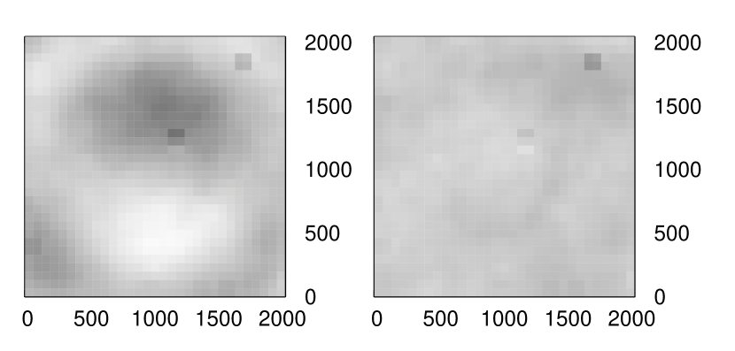
Figure 5.— The difference between the $Y$ coordinates of the transformed reference and the input star coordinates for a typical HAT field. The left panel shows the difference for fourth-order, the right panel for sixth-order polynomial fits.

As regards statistics, we performed the astrometry and source identification for 243,447 HAT images that had been acquired between the beginning of 2003 and June 2006. The wide-field telescopes observed 52 individual and almost non-overlapping fields between $b=-30^{\circ}$ and $b=+74^{\circ}$ galactic latitudes.

We initiated the processing with the following parameters. For the triangulation, the 3000 brightest sources were used from both the reference catalog and the detected stars. The critical unitarity was set to $0.01$, therefore if the fitted initial transformation had an unitarity larger than this value, the level of the triangulation expansion was increased. The final transformation was determined using a weighted sixth-order polynomial fit. Because the astrometric errors of brighter stars are smaller, we weighted data-points based on their magnitude during the fit. Finally, the maximal distance of matches was set to one pixel to reject false identifications.

Astrometry and cross-identification of sources was successful for 238,353 images. The remaining 5094 images were analyzed manually, and we found that only 13 of them were good enough to expect astrometry to succeed; all the other ones were cloudy or had shown various other errors. Astrometry on these 13 images also succeeded by decreasing the number of stars for triangulation to 2000. It means that a completely automatic run yielded 99.995% success rate, and the other images were also matched by applying small changes to the fine-tune parameters.

In order to test the algorithm with a different instrument, we also performed astrometry on 22,936 TopHAT images taken in 2005. The only difference in the procedure was that the polynomial transformation was only of 2nd order. The success ratio was 93%, but 90% of the frames where astrometry failed were cloudy with virtually no stars. Astrometry also failed on very short exposure (10sec) V-band frames. Fine-tuning the parameters (number of triangles, input lists) resolved most of these cases.

The following statistics was done on the wide-field HAT frames. The median value of the number of matched sources relative to the number of stars in the reference or the input list was $98.38\%\pm 0.31\%$ (median deviation). The average value of the CPU usage was $0.77\pm 0.22$ seconds per frame on a 64-bit AMD Opteron machine running at 2GHz. Astrometry was successful on 96.78% of the images using Delaunay-triangulation without extended triangles (CPU: 0.73sec), while 0.49% of the frames were processed at level $\ell=1$ extended triangulation (CPU: 1.79 sec), 0.06% at $\ell=2$ (CPU: 2.22 sec), 33 images at $\ell=3$ (CPU: 3.67 sec) and 1334+5094 images at $\ell=4$ extended triangulation (CPU: 5.20 sec). Here 5094 refers to those images were astrometry failed even at $\ell=4$, mostly because of bad data quality (see before). The reason for the Delaunay triangulation being successful for 96% of the wide-field HAT frames without extended triangulation is because the HAT instruments perform homogeneous data acquisition, and are very well characterized (zero-points, saturation). Thus, the 2MASS reference catalogs can be retrieved for the given field in such a way that there are many sources in common. In general applications, however, when the saturation limit and faint magnitude limits of an image have only a crude estimate, the extended triangulation is essential.

Although the procedure is fast, we note that the most time consuming part of the process is the triangulation generation and the triangle matching itself. On average, this required more than 60% of the total time, and at $\ell=4$, 92% of the time. The median value of the fit residuals was 0.06 pixels, while the median value of the unitarities was 0.0042. The latter is in a quite good agreement with the expected value of the nonlinearity factor $f_{d}\approx 0.005$.

4.3. Comparison with other implementations

We also compared the performance of the program grmatch with an existing implementation within IRAF, namely the images.immatch package with its relevant tasks xyxymatch, geomap and geoxytran. The steps of the point matching were as described in § 3.3. First, an initial set of possible pairs were established using xyxymatch and the “triangles” option as matching method. Because the triangle sets generated by xyxymatch are full triangulations, we limited our input lists to the brightest sources, otherwise the $\mathcal{O}(N^{3})$ dependence of the number of the triangles would have resulted in an unrealistically long matching time. Second, the initial transformation was fitted using geomap, and followed by transforming the reference catalog to the frame of the input list using geoxytran and this fit. Third, the transformed reference and the original input list were also matched by xyxymatch, but this time using the “tolerance” matching method. Finally, this new list of point pairs were used again to refine the geometrical transformation by geomap.

The comparison of grmatch and the IRAF images.immatch implementation was based on 950 individual images, all acquired by TopHAT from the same FOV. We note that we had to use the relatively narrow field TopHAT for the comparison, as the triangle match on the original 8.2° HATNet frames is almost hopeless given the spatial distortions, the large number of stars, and the difficulty to select the brightest stars and at the same time retain a small total number of selected sources (in order to be able to cope with a full triangulation). On each image there were approximately $800-900$ detected stars, depending on the airmass or thin clouds. For the triangulation and the initial xyxymatch fit we used the $35$ brightest sources both from the reference catalog and from the input star lists. We found that grmatch required $\sim 0.1$ sec CPU time on average while the whole procedure using these IRAF-based tasks, as described above, required $\sim 5-7$ sec net CPU time for a single image. Both algorithms yielded the same transformation coefficients and found the same number of pairs, however, in $3$ cases, the number of sources used for triangulation had to be increased manually to $40$ or $45$. It is noteworthy that although the IRAF version proved to be significantly slower, the time consuming part was the first xyxymatch matching. All other tasks, including the second matching (with “tolerance” option) required only a fraction of a second per image.

5. Summary

In this paper we present a robust algorithm for cross-matching two two-dimensional point lists. The task is twofold: finding the smooth spatial transformation between the lists, and cross-matching points. These two steps are intertwined, and are performed in an iterative way till satisfactory transformation and matching rate are reached. We make only very basic assumptions that hold for almost all astronomical applications, including wide-field surveys with distorted fields and large number of sources. Namely, the transformation between the point lists is dominantly a similarity transformation (arbitrary shift, rotation, magnification, inversion). A significant distortion term can be present, given it can be linearized on the scale-length of the average distance of neighboring points.

In § 2 we briefly described symmetric point-matching in one and two dimensions, because this tool is used throughout the astrometry procedure. Finding the initial transformation between the point lists is based on triangle matching. First we defined various normalized triangle spaces in § 3.1.1. The “mixed” triangle space of Valdes et al. (1995) is a continuous function of the triangle parameters, but flipped triangles are not distinguished. The “chiral” triangle space ensures that chirality information is preserved, but this space is not continuous. We showed that it is possible to define a “continuous” triangle space that is both continuous and preserves chirality, and which, furthermore, spans a larger volume and diminishes confusion of triangles having similar coordinates.

Taking into account the distortion of a field and the astrometric errors, we calculated both the optimal size and number of triangles. For the typical setup of a HATNet telescope ($8\arcdeg\times 8\arcdeg$ FOV, distortion factor $f_{d}\sim 0.005$) the optimal size is $0.2\arcdeg$, and the optimal number of triangles is less than $2\times 10^{6}$. We use Delaunay triangulation for generating the triangles of the triangle-space. This has the advantage of being fast, robust, and generating local triangles that are less prone to being distorted. In § 3.1.3 we noted, however, that Delaunay triangulation is sensitive for removing or adding points to the list, and thus instable. We introduced an extension of this triangulation that is parametrized by an $\ell$ level.

Having determined the transformation between the two lists, one can check how well our initial assumption of the dominant term being linear holds. In § 3.2 we introduced the unitarity of the transformation, a simple scalar measure of this property. We described the practical details of the algorithm in § 3.3, and the actual software implementation (grmatch, grtrans) in § 4.1.

Finally, we ran the above programs on some 240,000 frames taken by the wide-angle cameras of HATNet, plus 20,000 frames acquired by the TopHAT telescope. The success rate was very close to 100%, and the routines handled the various pointing errors, defocusing and 6th order distortions in the wide fields. Both programs will become available in binary format for a wide range of architectures upon request from the authors.

References

- Akerlof et al. (2000) Akerlof, C., et al.2000, AJ, 119, 1901
- Alonso et al. (2004) Alonso, R., et al.2004, ApJ, 613, L153
- Bakos (2002) Bakos, G. Á., Lázár, J., Papp, I., Sári, P., Green, E. M. 2002, PASP, 114, 974
- Bakos (2004) Bakos, G. Á., Noyes, R. W., Kovács, G., Stanek, K. Z., Sasselov, D. D. and Domsa, I. 2004, PASP, 116, 266
- Calabretta & Greisen (2002) Calabretta, M. R., Greisen, E. W. 2002, A&A, 395, 1077
- Charbonneau (2006) Charbonneau, D., Brown, T. M., Burrows, A., Laughlin, G. 2006, in Conference Proceedings of Protostars and Planets V, astro-ph/0603376
- Gionis (2002) Gionis, A.: Computational Geometry: Nearest Neighbor Problem (lecture notes) 666http://theory.stanford.edu/~nmishra/CS361-2002/lecture12-scribe.pdf
- Groth (1986) Groth, E. J. 1986, AJ, 91, 1244
- Hartman et al. (2004) Hartman, J. D., Bakos, G. Á., Stanek, K. Z., Noyes, R. W. 2004, AJ, 128, 1761
- Joye & Mandel (2003) Joye, W. A., Mandel, E. 2003, ASP Conf. Ser., 295, 489
- Mink (2002) Mink, D. J., 2002, ASP Conf. Ser, 281, 169
- Pepper, Gould, & Depoy (2004) Pepper, J., Gould, A., & Depoy, D. L.2004, AIP Conf. Proc. 713: The Search for Other Worlds, 713, 185
- Phillips & Davis (1995) Phillips, A. C., Davis, L. E. 1995, in Astronomical Data Analysis Software and Systems IV, ASP Conference Series Vol. 77, 297 (eds. R. A. Shaw, H. E. Payne and J. J. E. Hayes)
- Pojmanski (1997) Pojmanski, G. 1997, Acta Astronomica, 47, 467
- Press et al. (1992) Press, W. H., Teukolsky, S. A., Vetterling, W.T., Flannery, B.P. 1992, Numerical Recipes in C: the art of scientific computing, Second Edition, Cambridge University Press
- Shewchuk (1996) Shewchuk, R. J. 1996, in Applied Computational Geometry: Towards Geometric Engineering, ed. M. C. Lin & D. Manocha (Berlin: Springer), 1148, 203
- Shupe (2005) Shupe, D. L., Moshir, Mehdrdad, Li, J.; Makovoz, D., Narron, R., Hook, R. N., 2005, ASP Conf. Ser., 347, 491 777see also http://spider.ipac.caltech.edu/staff/shupe/distortion_v1.0.htm
- Skrutskie (2006) Skrutskie, M. F., Cutri, R. M., Stiening, R., Weinberg, M. D., Schneider, S., Carpenter, J. M., Beichman, C., Capps, R., Chester, T., Elias, J., Huchra, J., Liebert, J., Lonsdale, C., Monet, D. G., Price, S., Seitzer, P., Jarrett, T., Kirkpatrick, J. D., Gizis, J., Howard, E., Evans, T., Fowler, J., Fullmer, L., Hurt, R., Light, R., Kopan, E. L., Marsh, K. A.,, McCallon, H. L., Tam, R., Van Dyk, S., and Wheelock, S., AJ, 131, 1163
- Stetson (1989) Stetson, P. B. 1989, in Advanced School of Astrophysics, Image and Data Processing/Interstellar Dust, ed. B. Barbury, E. Janot-Pacheco, A. M. Magalhães and S. M. Viegas (São Paulo, Instituto Astrônomico e Geofísico)
- Valdes et al. (1995) Valdes, F. G., Campusano, L. E., Velásquez, J. D., Stetson, P. B. 1995, PASP, 107, 1119
- Thiebaut & Boër (2001) Thiebaut, C., Boër, M. 2001, ASP Conf. Ser., 238, 388