Deep FORS1 observations of the double Main Sequence of $\omega$ Centauri

Abstract

We present the results of a deep photometric survey performed with FORS1@VLT aimed at investigating the complex Main Sequence structure of the stellar system $\omega$ Centauri. We confirm the presence of a double Main Sequence and identify its blue component (bMS) over a large field of view up to 26’ from the cluster center. We found that bMS stars are significantly more concentrated toward the cluster center than the other ”normal” MS stars. The bMS morphology and its position in the CMD have been used to constrain the helium overabundance required to explain the observed MS morphology.

1. Introduction

The understanding of the origin and evolution of the stellar system $\omega$ Centauri (NGC5139) still represents one of the most intriguing unanswered questions of stellar astrophysics. Unique among Galactic star clusters in terms of structure, kinematics and stellar content, it is the only known globular cluster (GC) which shows a clear metallicity spread (Norris et al. 1996 and references therein). Recent photometric surveys have revealed the presence of multiple sequences in its color-magnitude diagram (CMD). In particular, high-precision photometric analyses have revealed a discrete structure of its red giant branch (RGB, Rey et al. 2004; Sollima et al. 2005a), indicating a complex star formation history. Beside the dominant metal-poor population (MP, ${\rm[Fe/H]}\sim-1.6$), three metal-intermediate (MInt) components (spanning a range of metallicity $-1.3<{\rm[Fe/H]}<-1.0$) and an extreme metal-rich population (${\rm[Fe/H]}\sim-0.6$, Pancino et al. 2002) have been identified. The different RGB populations of $\omega$ Cen share different structural and dynamical properties (Norris et al. 1997; Ferraro et al. 2002; Pancino et al. 2003; Sollima et al. 2005a). In particular, Norris et al. (1997) found that the 20 % metal-rich tail of the distribution is more concentrated toward the cluster center than the dominant metal-poor component.

Finally, Anderson (2002) and Bedin et al. (2004) discovered new peculiarities also along the Main Sequence (MS) of the cluster. Indeed, an additional blue MS (bMS, comprising $\sim$ 30% of the whole cluster MS stars) running parallel to the dominant one, has been resolved. According to stellar models with canonical chemical abundances, the location of the observed bMS would suggest a very low metallicity ($[Fe/H]<-2$). Conversely, the spectroscopic analysis of a sample of MS stars belonging to the two MS components showed that bMS stars present a metallicity $\sim 0.3~{}dex$ higher than that of the dominant cluster population (Piotto et al. 2005). Norris (2004) suggested that a large helium overabundance ($\Delta Y\sim 0.15$) could explain the anomalous position of the bMS in the CMD. However, such a large helium abundance spread poses serious problems in the overall interpretation of the chemical enrichment history of this stellar system.

In this paper we present deep BR photometry covering a wide area extending from 6’ to 26’ from the cluster center with the aim of studying the morphology, the radial extent and the distribution of the bMS population.

2. Observations and data reduction

The photometric data were obtained with the FORS1 camera, mounted at the Unit1 (UT1) of the ESO Very Large Telescope (VLT, Cerro Paranal, Chile). Observations were performed during 6 nights on March and April 2005 (see Table 1), using the standard resolution mode of FORS1. In this configuration the image scale is 0.2” $pixel^{-1}$ and the camera has a global field of view of $6.8^{\prime}\times 6.8^{\prime}$ . A mosaic of 8 partially overlapping fields spanning a wide area from 6’ to 26’ from the cluster center were observed (see Fig. 1). The innermost field partially overlaps the deep ACS photometry described in Ferraro et al. (2004) allowing linkage between the two datasets. The standard pre-reduction procedure was followed to remove the bias and to apply flat-field corrections. We used the point-spread-function (PSF) fitting package DoPhot (Schechter et al. 1993) to obtain instrumental magnitudes for all the stars detected in each frame. For each field, two different frames were observed through the B and R filters. The photometric analysis was performed independently on each image. Only stars detected in all the four frames were included in the final catalog. For each passband, the obtained magnitudes were transformed to the same instrumental scale and averaged. As usual, the most isolated and brightest stars in the field were used to link the aperture magnitudes to the fitting instrumental ones, after normalizing for exposure time and correcting for airmass. During the observing run, nine standard stars from the Landolt (1992) list were observed. Aperture photometry was performed on each standard, and used to derive the equations linking the aperture photometry to the standard photometric system. The calibration equations linking the b and r instrumental magnitudes to the standard system ones (B and R) are:

$$B-b=-0.067~{}(b-r)+27.123$$

$$R-r=0.007~{}(b-r)+27.400$$

Both the slope and the zero points of the above relations are in good agreement with those provided by the FORS1 support team. Finally, a catalog with more than 70,000 calibrated stars was produced.

3. Color Magnitude Diagram

Fig. 2 shows the (R, B-R) CMD of the entire sample. As can be seen, the unevolved population of $\omega$ Cen down to $R\sim 24$ is sampled. In particular, two different MS populations can be identified:

• The dominant MS population (rMS) containing $\sim 75\%$ of the entire MS population stars;

• A narrow blue MS, running parallel to the rMS population, can be distinguished at $19.5<R<21$.

In order to investigate the morphology and properties of the bMS, we studied the distance distribution of bMS stars from the mean ridge line of the rMS. The rMS mean ridge line was computed by selecting by eye the stars belonging to the dominant MS component. We took care in excluding both blue objects populating the faint part of the CMD (i.e. white dwarfs) and the bright red population (mostly due to the Galactic field). Particular care was taken in excluding bMS stars which could contaminate the selected rMS sample. However, bMS stars are well separated from the rMS over a large magnitude range. We estimate the contamination from bMS stars to be $<10$% between $19<R<21$, with negligible impact on the ridge line determination. Then, we fitted the selected stars with a low-order polynomial and rejected stars lying at a $>~{}2\sigma$ distance. The procedure was iterated until convergence to a stable fit was obtained. Then, we defined the observable $\Delta x$ as the geometrical distance of each MS star from the reference ridge line. Fig. 3 shows the obtained mean ridge line and the distance distributions in the $left$ and $middle~{}panels$, respectively. In the $right~{}panel$ the histograms of the distances from the mean ridge line at different magnitude levels are shown. As can be noted, the bMS appears distinguishable from the rMS at magnitude $R\sim 19.2$, reaching a maximum separation from the rMS at $R\sim 20.3$ . The bMS merges into the bulk of the cluster MS at a fainter magnitude ($R\sim 21.3$). Fig. 4 shows the CMD for each of the eight fields observed in the present analysis. The CMDs related to the innermost fields are significantly less populated than the outer ones. This effect is due to the presence of many bright saturated stars that cover most of the chip field of view thus allowing a meaningful photometric analysis only over a small fraction of the chip area. As can be seen, the MS splitting is visible in all the CMDs regardless of the distance from the cluster center. This evidence indicates that bMS stars cover the entire extension of the cluster, being part of the population mix of $\omega$ Cen. The evident MS splitting clearly visible in Fig. 2, 3 and 4 confirms what already found by Anderson (2002) and Bedin et al. (2004) on the basis of high-precision HST photometric studies performed on two small fields located in a peripheral region of the cluster (at $\sim$ 7’ and 17’ from the cluster center, respectively). However, this is the first time that the bMS is identified over such a large area. This allowed us to perform a meaningful comparison between the bMS and rMS radial distributions.

4. Radial Distributions

In order to derive the radial distributions of the two MS populations, we selected the samples of bMS and rMS stars on the basis of the distances from the mean ridge line of the rMS shown in the $middle~{}panel$ of Fig. 3 . The adopted selection boxes for the two MS components are shown in Fig. 5 . Only stars in the magnitude range $19.4<R<20.8$ have been used, in order to limit the analysis to the region in which the two MS components are more clearly distinguished. For the rMS sample only stars with $-0.05<\Delta x<0.2$ have been considered, while bMS stars were selected among stars with $-0.17<\Delta x<-0.08$. On the basis of these selection criteria we isolated 7,122 rMS and 1,718 bMS stars. A residual contamination of rMS stars can be still present in the bMS selection box. This effect could be important expecially in the innermost fields, where severe crowding produces large uncertainties in magnitude and color. In order to quantify this effect, we performed an extensive set of experiments with artificial stars (Bellazzini et al. 2002): a sample of 100,000 artificial stars whose magnitude were extracted from the rMS mean ridge line have been simulated in the observed fields. The spread of the distribution around the rMS mean ridge line reflects the photometric errors in the different regions of the cluster. Then, we counted the number of stars that satisfy the bMS selection criterion and evaluated the contamination factor. The above analysis indicated that $\sim 7$% of the bMS stars in the inner 12’ are expected to be spurious rMS stars. The contamination decreases rapidly at larger radii, becoming neglegible at $r>16^{\prime}$. We took into account this effect in the following analysis.

Fig. 6 shows the cumulative radial distribution of the rMS and bMS samples. The comparison indicates that the two MS components of $\omega$ Cen are distributed in a different way. A two-dimensional generalization of the Kolmogorov-Smirnov test (Peacock 1983, Fasano & Franceschini 1987) gives a probability that the spatial distribution of the bMS sample and the rMS one are drawn from the same parent distribution of less than $10^{-6}$. In particular, bMS stars are more concentrated toward the cluster center. To further investigate this effect, we computed the ratio between the number of bMS and rMS stars at different distances from the cluster center. This observable is insensitive to the photometric completeness and it could provide important information on the relative frequency of bMS stars. Fig. 7 shows the calculated ratio corrected for contamination effects (see above) as a function of the distance from the cluster center. On average, the bMS accounts for $\sim 24$% of the whole MS population. As can be noted, the relative fraction of bMS-to-rMS stars decreases from 0.28 (at distances $\sim 7^{\prime}$) to 0.15 (at distances $>19^{\prime}$). This is best put into evidence in Fig. 8 where the distribution of MS stars with respect to the rMS mean ridge line, calculated in the magnitude range $19.4<R<20.8$ for stars at three different distances from the cluster center, is shown.

5. Comparison with Theoretical Isochrones

Apart from the HB, the MS is the most helium-sensitive region of the CMD. A significant helium overabundance could explain the anomalous location of the bMS in the CMD because of the effect on the mean opacity that leads stars to higher temperatures and bluer colors (Norris 2004). The relative location of the two MS components shown in the CMD of Fig. 2 allowed us to infer an indirect estimate of the helium content of the bMS population by means of a detailed comparison with suitable theoretical models. In doing this, we used a new set of theoretical isochrones calculated adopting the most up-to-date input physics and spanning a wide range in helium abundance. A detailed description of the evolutionary code used to compute these new models can be found in Straniero et al. 1997. To compare the observed CMD with theoretical isochrones, a distance modulus and a reddening correction have to be adopted. In the following we used $(m-M)_{0}=13.70\pm 0.13$ (Bellazzini et al. 2004). Concerning the reddening and extinction coefficients, we used $E(B-V)=0.11\pm 0.01$ (Lub 2002), $A_{B}=4.1~{}E(B-V)$, $A_{R}=2.32~{}E(B-V)$ (Savage & Mathis 1979).

For the dominant rMS population we adopted a metallicity of $[Fe/H]=-1.6$ as suggested by the most extensive spectroscopic surveys performed on giant stars (Norris et al. 1996; Suntzeff & Kraft 1996), while for the bMS we adopted a significantly higher metallicity of $[Fe/H]=-1.3$, as indicated by Piotto et al. (2005). The contribution of the $\alpha$-element enhancement has been taken into account by simply rescaling standard models to the global metallicity [M/H], according to the following relation

$$\mathrm{[M/H]}~{}=~{}\mathrm{[Fe/H]}+\log_{10}(0.638~{}10^{[\alpha/Fe]}+0.362)~{}~{}~{}~{}~{}\mbox{Salaris et al. (1993)}$$

We adopted $[\alpha/Fe]=+0.3$ for both the rMS and the bMS samples, according to the most recent high-resolution spectroscopic results (Norris & Da Costa 1995; Smith et al. 2000; Vanture et al. 2002). For the two MS components we computed a set of models with canonical helium abundance (Y=0.246, Salaris et al. 2004) and various helium enhancement levels. The metallicity, in terms of mass fraction Z, has been calculated according to the relation

$$Z=(1-Y)\frac{10^{[M/H]+log[Z/X]_{\odot}}}{1+10^{[M/H]+log[Z/X]_{\odot}}}~{}~{}~{}~{}~{}~{}~{}~{}~{}~{}\mbox{Sollima et al. (2005b)}$$

where $[Z/X]_{\odot}=0.0176$, according to Lodders et al. (2003). Fig. 9 shows the isochrone fitting for the two observed MS populations of $\omega$ Cen. As can be seen the metal-poor isochrone nicely fits the rMS. While the metal-rich isochrone with cosmological helium abundance cannot reproduce the location of the bMS in the CMD, a significant helium enhancement ($Y>0.35$) is required to reproduce the bMS. The bMS is best fitted by an isochrone with Y=0.40 . This value is in good agreement with that predicted by Norris (2004) and that estimated by Piotto et al. (2005) on the basis of ACS observations of a peripheral region of the cluster. However, the exact amount of helium overabundance needed to explain the observed MS morphology is still largely uncertain because of the following reasons:

• Uncertainties in the color-temperature conversion. A helium overabundance significantly alters the trasparency of the atmosphere. The adoption of color-temperature conversion based on standard models with no helium overabundance produces a shift in color that mimics a larger helium abundance;

• Uncertainties on the metal abundances. Small changes in the iron and/or $\alpha$-elements abundances produce significant effects on the MS morphology. Theoretical models indicate that a variation of $\Delta Z=0.0001$ in the metal content difference between the two MS populations would mimic the effect of a change of $\Delta Y=0.012$ in the deduced helium abundance;

• Theoretical uncertainties in the helium-rich isochrones. Until now, none of the known stellar systems has been found to have a helium abundance $Y>0.30$ . Therefore, there are no direct observational constraints that allow to confirm the effect of the large helium overabundance predicted by theoretical models.

In Fig. 10 we compare the CMD of Fig. 2 with a synthetic CMD obtained adopting for the two MS components the stellar parameters listed above, a Salpeter (1955) Initial Mass Function and photometric errors derived from the arificial star technique described in Sect. 4 . Note that the synthetic CMD reproduces quite well the observed CMD also in the faint part of the MS where the bMS merges with the rMS at $R\sim 21$ . The effective temperature of the lower part of the MS is indeed less sensitive to a variation of the helium content with respect to the upper part (see Alexander et al. 1997). This occurrence can be explained with simple arguments. In very low mass stars ($<0.5M_{\odot}$), the onset of the $H_{2}$ recombination (below 6000 K) induces the formation of a deep convective envelope characterized by a very efficient energy transport. In practice, the temperature gradient coincides with the adiabatic gradient up to the top of the convective zone. In this condition, since the radiative flux is negligible, the effective temperature is mainly controlled by the details of the equation of state and it is less sensitive to the variation of the radiative opacity. In particular, the adiabatic gradient is dominated by the presence of hydrogen molecules, while the atomic H and He only give minor contributions. Indeed, owing to the presence of these molecules, the number of internal degrees of freedom increases, the specific heat increases and the adiabatic gradient significantly decreases with respect to the typical value of a monoatomic perfect gas (with just 3 degrees of freedom and $dlogT/dlogP=0.4$). Detailed stellar models calculations confirm that the separation between isochrones computed with different helium abundances becomes progressively less evident at fainter magnitudes. The increasing photometric error introduces a further confusion at lower magnitudes making impossible to distinguish the two MSs.

6. Discussion and Conclusions

The results presented in this paper indicate that the bMS presents peculiar structural properties which differ from those of the dominant MS population of $\omega$ Cen. In particular, bMS stars are significantly more concentrated toward the cluster center. Note that differences in the spatial distribution of different RGB populations were already found by Norris et al. (1997), Pancino et al. (2003) and Sollima et al. (2005a) which showed that the metal-rich ($[Fe/H]>-1.4$) stellar populations of $\omega$ Cen are more concentrated than the dominant metal-poor population. Peculiarities in the radial distributions were also found among the HB stars of $\omega$ Cen: Bailyn et al. (1992) and Rey et al. (2004) showed that the population of Extreme Horizontal Branch (EHB) stars of $\omega$ Cen is more concentrated toward the cluster center than MS and Sub Giant Branch (SGB) stars.

A detailed comparison with theoretical isochrones confirms that a significant helium overabundance ($\Delta Y>0.10$) could explain the observed bMS morphology, as already suggested by Norris (2004), Piotto et al. (2005) and Lee et al. (2005). Note that the existence of a stellar population with such a large helium overabundance can also naturally explain the HB morphology (in particular the existence of the population of EHB stars observed in the cluster, Lee et al. 2005), the location of the RGB bumps (Sollima et al. 2005a) and the SGB morphology (Sollima et al. 2005b) remaining consistent with the short ($<2Gyr$) star formation time-scale estimated by Sollima et al. (2005b). The peculiar structural properties of the bMS indicate that the star formation process in $\omega$ Cen could have proceeded favoring the formation of helium-rich population(s) in the inner region of the cluster.

However, this scenario poses serious problems in drawing the overall chemical enrichment history of this stellar system. In fact, none among the known chemical enrichment mechanisms is able to produce the huge amount of helium required to reproduce the observed MS morphology without drastically increasing the metal abundance. Indeed, the derived helium-to-metals abundance gradient between the dominant metal-poor and bMS population turns out to be $\delta Y/\delta Z>>100$, in stark contrast with more canonical values of $\delta Y/\delta Z\sim 3-4$ (Jimenez et al. 2003). In this respect, an intriguing puzzle is presented by the observed incongruences between the expected and the observed luminosity of metal-intermediate ($[Fe/H]\sim-1.2$) RR Lyrae found in $\omega$ Cen by Sollima et al. (2006, see also Rey et al. 2000 and Norris 2004). Note that a helium-rich population is not expected to produce a sizeable RR Lyrae component (Lee et al. 2005). Hence, two populations with similar metallicities but very different helium abundances seem to coexist within the cluster.

A selective self-enrichment process has to be invoked in order to produce the required amount of helium while keeping the metal abundance practically unchanged. Moreover, a very efficient mechanism is required in order to homogenize and efficiently re-use all the “enriched” material ejected by the previous generation of polluting stars.

However, a pure self-enrichment scenario may not be the best description of the evolution of $\omega$ Cen. Alternative scenarios can also be considered.

In particular, the bMS population could have formed in a different environment, thus not partaking in the chemical enrichment process of $\omega$ Cen. In this case, a complex interplay of chemical and dynamical evolution has to be taken into account, including gas exchange with the Milky Way and/or minor mergers, within a framework such as the binary cluster mergers scenario (Makino et al. 1997; Minniti et al. 2004).

Bekki & Norris (2006) noted that the large fraction of bMS stars ($\sim 24$%) cannot be explained without assuming that most of the helium enriched gas necessary to form the bMS originated from external sources. They suggested that part of the helium-enriched stars formed from gas ejected by field stellar populations surrounding $\omega$ Cen when it was the nucleus of an ancient dwarf galaxy, and later fell into the central region of the system.

Another possible explanation can be provided by the presence of spatial variation in the helium abundance of the protostellar clouds from which the helium-rich population(s) of $\omega$ Cen formed. Diffusion could produce such an effect as a result of the different acceleration imparted to helium atoms because of their different atomic masses (Chuzhoy 2006).

Table 1Observing logs

Field	Date	Filter	Exp time
			sec
1	10 Apr 2005	B	1099
1	10 Apr 2005	B	1099
1	10 Apr 2005	R	394
1	10 Apr 2005	R	394
2	16 Mar 2005	B	1099
2	16 Mar 2005	B	1099
2	16 Mar 2005	R	394
2	16 Mar 2005	R	394
3	16 Mar 2005	B	1099
3	16 Mar 2005	B	1099
3	16 Mar 2005	R	394
3	16 Mar 2005	R	394
4	08 Apr 2005	B	1099
4	08 Apr 2005	B	1099
4	08 Apr 2005	R	394
4	08 Apr 2005	R	394
5	10 Apr 2005	B	1099
5	10 Apr 2005	B	1099
5	10 Apr 2005	R	394
5	10 Apr 2005	R	394
6	12 Apr 2005	B	1099
6	12 Apr 2005	B	1099
6	12 Apr 2005	R	394
6	12 Apr 2005	R	394
7	04 Apr 2005	B	1099
7	04 Apr 2005	B	1099
7	04 Apr 2005	R	394
7	04 Apr 2005	R	394
8	12 Apr 2005	B	1099
8	12 Apr 2005	B	1099
8	12 Apr 2005	R	394
8	12 Apr 2005	R	394

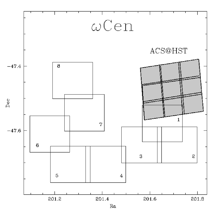
Figure 1.— Map of the region sampled by the FORS1 observations. North is up, east on the right. The eight fields observed with FORS1 are shown. Grey boxes indicate the position of the ACS photometry by Ferraro et al. (2004). The cluster center is located in the central ACS field.

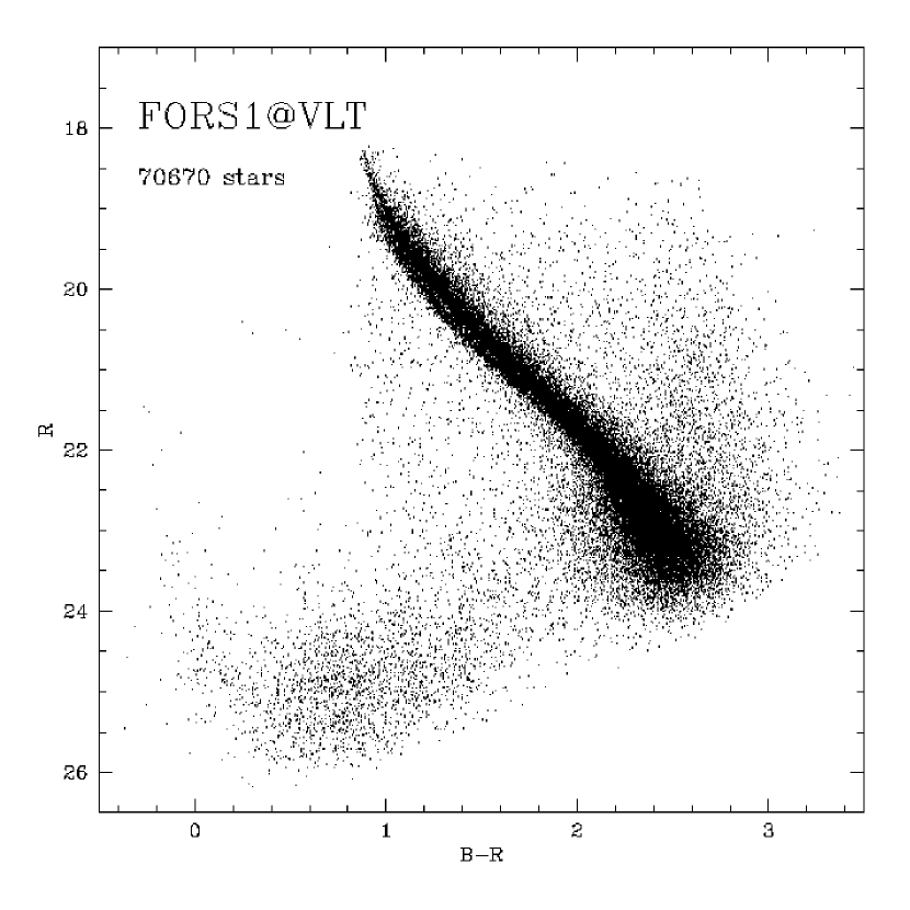
Figure 2.— R, B-R CMD for the global sample of $\sim$70,000 stars measured in $\omega$ Cen.

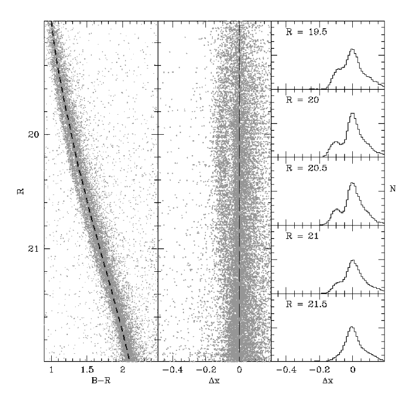
Figure 3.— The zoomed (R, B-R) CMD of $\omega$ Cen in the bMS region is shown in the $left~{}panel$. The mean ridge line of the rMS population is overplotted to the CMD as a dashed line. The distribution of MS stars with respect to the reference mean ridge line is shown in the $middle~{}panel$. In the $right~{}panel$ the histograms of the distances from the mean ridge line at different magnitude levels are shown.

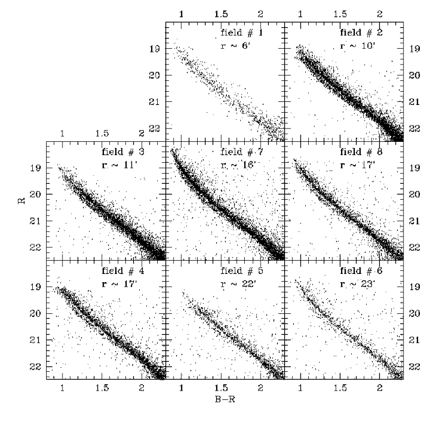
Figure 4.— The (R, B-R) CMDs of $\omega$ Cen zoomed in the bMS region for each of the eight observed fields. The field numbers are the same of Fig. 1 .

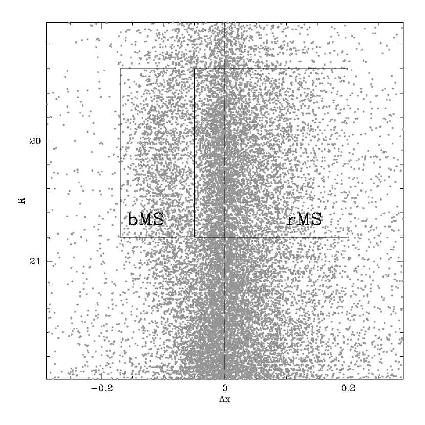
Figure 5.— Selection boxes for the rMS and bMS population in the ($\Delta x$,R) plane ($Middle~{}panel$ of Fig. 3) .

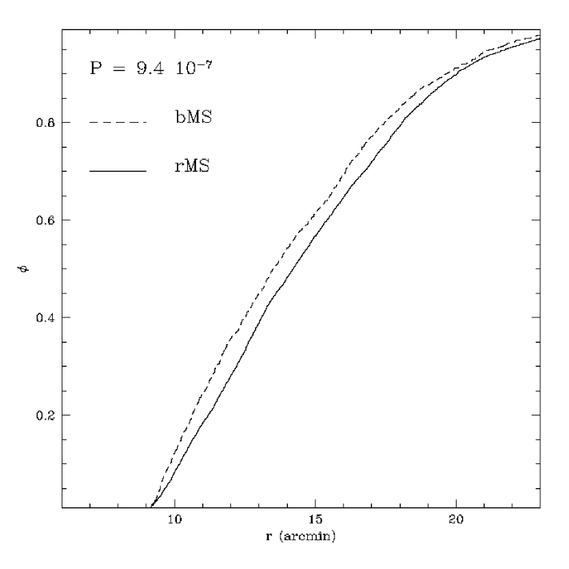
Figure 6.— Cumulative radial distribution for the rMS stars (solid line) and bMS stars (dashed line) as a function of their projected distance from the cluster center.

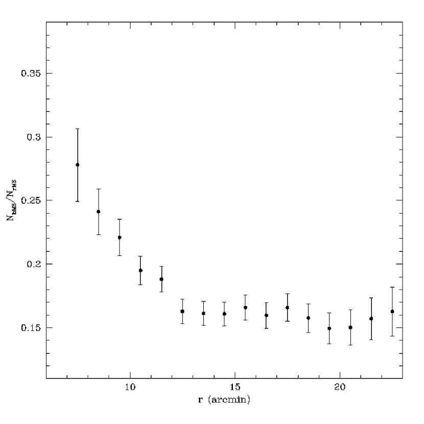
Figure 7.— Corrected ratio between the number of bMS and rMS stars at different distances from the cluster center.

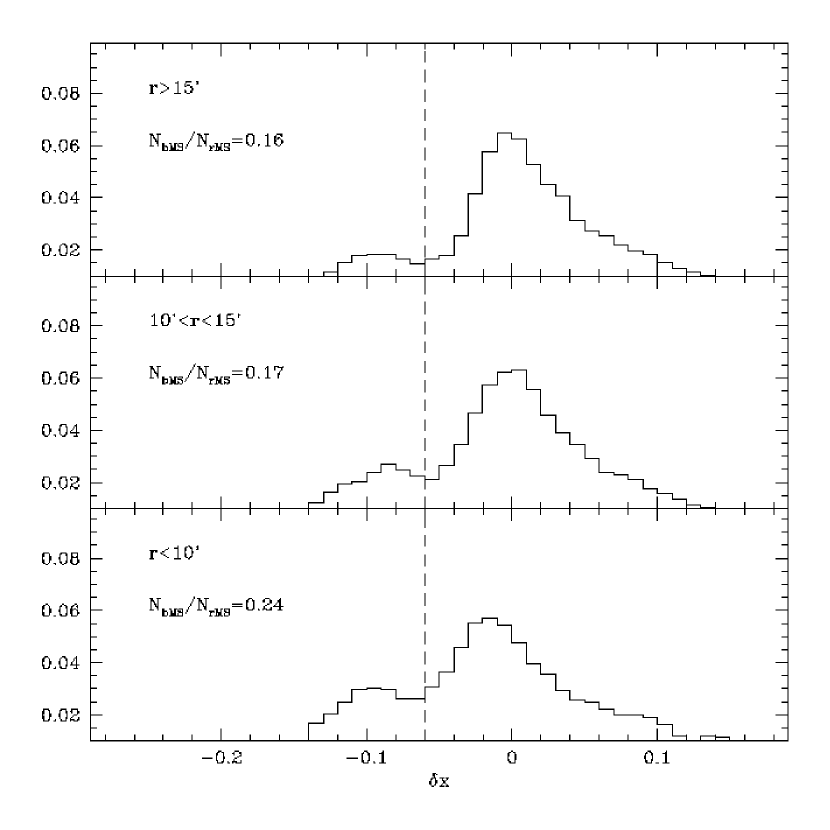
Figure 8.— Distribution of MS stars with respect to the reference mean ridge line calculated in the magnitude range $19.4<R<20.8$ for stars at distance $r<10^{\prime}$ (bottom $panel$), $10^{\prime}<r<15^{\prime}$ (middle $panel$) and $r>15^{\prime}$ (top $panel$) from the cluster center.

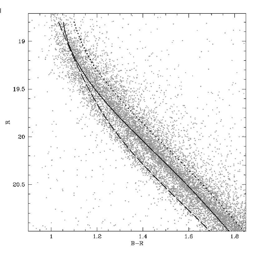
Figure 9.— Isochrone fitting of the MS populations of $\omega$ Cen. Theoretical isochrones with appropriate metallicity and helium abundance ([Fe/H]=-1.6 ; Y=0.246: solid line, [Fe/H]=-1.3 ; Y=0.246:dotted line , Y=0.40: dashed line) are overplotted.

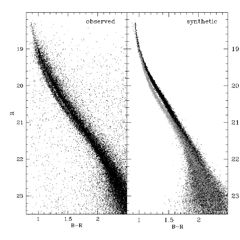
Figure 10.— Comparison between the observed (R, B-R) CMD of $\omega$ Cen (left $panel$) with a synthetic CMD (right $panel$). Black points simulate stars with [Fe/H]=-1.6 and Y=0.246, grey points simulate stars with [Fe/H]=-1.3 and Y=0.40 .

References

- Alexander et al. (1997) Alexander, D. R., Brocato, E., Cassisi, S., Castellani, V., Ciacio, F., Degl’Innocenti, S., 1997, A&A, 317, 90
- Anderson (2002) Anderson J. in ” Centauri: A Unique Window into Astrophysics”, 2002, ed. F. van Leeuwen, J. D. Huges & G. Piotto, ASP Conf.Series, 87
- Bailyn et al. (1992) Bailyn, C. D., Sarajedini, A., Cohn, H., Lugger, P. & Grindlay, J. E., 1992, AJ, 103, 1564
- Bedin et al. (2004) Bedin, L. R., Piotto, G., Anderson, J., Cassisi, S., King, I. R., Momany, Y. & Carraro, G., 2004, ApJ, 605, L125
- Bekki & Norris (2006) Bekki, K. & Norris, J. E., 2006, ApJ, 637, L109
- Bellazzini et al. (2002) Bellazzini, M., Ferraro, F. R., Origlia, L., Pancino, E., Monaco, L., Oliva, E., 2002, AJ, 124, 3222
- Bellazzini et al. (2004) Bellazzini, M., Ferraro, F. R., Sollima, A., Pancino, E., Origlia, L., 2004, A&A, 424, 199
- Chuzoy (2006) Chuzoy, L., 2006, MNRAS, in press
- Fasano & Franceschini (1987) Fasano, G. & Franceschini, A., 1987, MNRAS, 225, 155
- Ferraro et al. (2002) Ferraro, F. R., Bellazzini, M., Pancino, E., 2002, ApJ, 573, 95
- Ferraro et al. (2004) Ferraro, F. R., Sollima, A., Pancino, E., Bellazzini, M., Origlia, L., Straniero, O., & Cool, A., 2004, ApJ, 603, L81
- Jimenez et al. (2003) Jimenez, R., Flynn, C., McDonald, J. & Gibson, B. K., 2003, Science, 299, 1552
- (13) Landolt, A. 1992, AJ, 104, 340
- Lee et al. (2005) Lee, Y. W. et al., 2005, ApJ, 621, L57
- (15) Lodders, K. 2003, ApJ, 591, 1220
- (16) Lub, J. 2002, in A Unique Window into Astrophysics, ed. F. van Leeuwen, J. D. Hughes, & G.Piotto, ASP Conf.Series, Vol. 265, 95
- (17) Makino, J., Akiyama, K., Sugimoto, D., 1997, Ap&SS, 185, 63
- (18) Minniti, D., Rejkuba, M., Funes, S. J., Jos G., & Kennicutt, R. C., 2004, ApJ, 612, 215
- Norris & Da Costa (1995) Norris, J. E., Da Costa, G. S., 1995, ApJ, 447, 680
- Norris et al. (1996) Norris, J. E., Freeman, K. C. & Mighell, K. J., 1996, ApJ, 462, 241
- Norris et al. (1997) Norris, J. E., Freeman, K. C., Mayor, M.& Seitzer, P., 1997, ApJ, 487, L187
- Norris (2004) Norris, J. E., 2004, ApJ, 612, L25
- Pancino et al. (2002) Pancino, E., Pasquini, L., Hill, V., Ferraro, F. R. & Bellazzini, M., 2002, ApJ, 568, L101
- Pancino et al. (2003) Pancino, E., Seleznev, A., Ferraro, F. R., Bellazzini, M. & Piotto, G., 2003, MNRAS, 345, 683
- Peacock (1983) Peacock, J. A., 1983, MNRAS, 202, 615
- Piotto et al. (2005) Piotto, G. et al., 2005, ApJ, 621, 777
- Rey et al. (2000) Rey, S.-C., Lee, Y.-W., Joo, J.-M., Walker, A., & Baird, S., 2000, AJ, 119, 1824
- Rey et al. (2004) Rey, S. C., Lee, Y. W., Ree, C. H., Joo, J. M., Sohn, Y. J. & Walker, A. R., 2004, AJ, 127, 958
- Salaris, Chieffi & Straniero (1993) Salaris, M., Chieffi, A., Straniero, O., 1993, Mem. Soc. Astron. Italiana, 63, 315
- Salaris et al. (2004) Salaris, M., Riello, M., Cassisi, S. & Piotto, G., 2004, A&A, 490, 911
- Salpeter (1955) Salpeter, E. E., 1955, ApJ, 121, 161
- Savage & Mathis (1979) Savage, B. D., Mathis, J. S., 1979, ARA&A, 17, 73
- Schechter et al. (1993) Schechter, P. L., Mateo, M., Saha, A., 1993, PASP, 105, 1342
- Smith et al. (2000) Smith, V. V., Suntzeff, N. B., Cunha, K., Gallino R., Busso, M., Lambert, D. L. & Straniero, O., 2000, AJ, 119, 1239
- Sollima et al. (2005a) Sollima, A., Ferraro, F. R., Pancino E., & Bellazzini, M. 2005a, MNRAS, 357, 265
- Sollima et al. (2005b) Sollima, A., Pancino E., Ferraro, F. R., Bellazzini, M., Straniero, O. & Pasquini, L., 2005b, ApJ, 634, 332
- Sollima et al. (2006) Sollima, A., Borissova, J., Catelan, M., Smith, H. A., Minniti, D., Cacciari, C. & Ferraro, F. R., 2006, ApJ, 640, L43
- Straniero, Chieffi & Limongi (1997) Straniero, O., Chieffi, A. & Limongi, M., 1997, ApJ, 490, 425
- Suntzeff & Kraft (1996) Suntzeff, N. B. & Kraft, R. P., 1996, AJ, 111, 1913
- van Leeuwen & Le Poole (2002) van Leeuwen, F. & Le Poole, R. S., 2002, in ” Centauri: A Unique Window into Astrophysics”, ASP Conf. Series, 265, 41
- Vanture et al. (2002) Vanture, A. D., Wallerstein, G. & Suntzeff, N. B., 2002, ApJ, 569, 984