Theoretical aspects of relativistic spectral features

Abstract

The inner parts of black-hole accretion discs shine in X-rays which can be monitored and the observed spectra can be used to trace strong gravitational fields in the place of emission and along paths of light rays. This paper summarizes several aspects of how the spectral features are influenced by relativistic effects. We focus our attention onto variable and broad emission lines, origin of which can be attributed to the presence of orbiting patterns – spots and spiral waves in the disc. We point out that the observed spectrum can determine parameters of the central black hole provided the intrinsic local emissivity is constrained by theoretical models.

1 Introduction

During the last four decades a picture of galactic nuclei has emerged in which massive black holes reside in the centre. In active galactic nuclei (AGN) accretion discs form around the core and provide most of the radiation emerging from that region. According to this scheme, intense X-rays originate just a few gravitational radii from the black hole horizon. Manifestation of strong gravity has been searched in X-ray spectra of AGN with the main aim of finding the firm evidence for the central black hole (BH) and determining its parameters, namely, mass and angular momentum (for a detailed exposition of the subject, see Peterson 1997; Krolik 1999).

Broad spectral features have been expected in X-rays on the basis of the model in which the iron line is formed on the surface of a geometrically thin, optically thick and relatively cold medium after irradiation by a primary source (Fabian et al. 1989). Nowadays, the general relativistic (GR) iron line profiles provide a powerful tool to measure the mass of the black hole in AGN as well as Galactic black-hole candidates. Blandford & McKee (1982) and Stella (1990) have developed the reverberation technique that employs a response of the line profile following variations of the illuminating primary source. Along the same line of thought, Matt & Perola (1992) proposed to employ variations of the time-integrated line properties – equivalent width, centroid energy and the line width. The method was developed further by many authors (see Fabian et al. 2000; Reynolds & Nowak 2003 for reviews and references). Apart from the mass $M_{\bullet}$, the main parameters of these models are the functional dependency of the intrinsic emissivity over the disc surface, $I(r)$, the specific angular momentum $a$ of the black hole and the inclination $\theta_{\mathrm{o}}$ of the accretion disc with respect to observer’s line of sight. High resolution in spectral and time domains is crucial to accomplish the analysis.

This paper concentrates on gravitational effects that act on the spectral features by smearing them and moving them among energy bins. In this way gravity exerts the influence on the ultimate form of the observed spectrum. We start with a brief summary of the equations describing intensity (and polarization) propagation in the field of a black hole. Detailed exploration of broad spectral features can be considered as a method complementary to studying the overall X-ray continuum (Shaffee et al. 2006) on one side and narrow spectral features (Turner et al. 2004) on the other extreme.

Relativistic effects are often discussed in terms of geometrical optics with photons travelling through the empty spacetime – this formulation is suited quite well to various flavours of ‘hot spots’ on the disc surface, but plasma exists also above the disc where it influences the observed signal to a certain degree. Theoretical approaches have been developed that can tackle more complicated situations, such as the case of dispersive media which may be able to address, more accurately, simultaneous observations in mutually remote parts of the electromagnetic spectrum.

In the second part of the paper we discuss flares and spots as a model for X-ray variability: multiple spots are created on the surface of an accretion disc following the intense irradiation. The observed signal is then modulated by relativistic effects. This scheme is testable and it captures many properties of present observations.

Mean spectra of orbiting spots resemble those of axisymmetric rings and we briefly discuss this degeneracy. It is inherent to time integrated data and can be resolved by increasing sensitivity and time resolution of the observations.

In the present context, the spots represent any kind of localized non-axisymmetric features residing on the disc surface, sharing its orbital motion and modulating the signal. They are thought to result from the illumination of a relatively cold gas of the disc after magnetic reconnection events. Such a possibility was proposed for the X-ray emitting region by Galeev et al. (1979) and developed in many papers (Poutanen & Fabian 1999; Merloni & Fabian 2001; Życki 2002; Czerny et al. 2004, and references cited therein).

The flare/spot scenario can be considered as a generalized model of the phenomenological lamp-post geometry where a point-like X-ray source is located at a specified height on the disc axis (Henri & Pelletier 1991; Martocchia & Matt 1996). Martocchia et al. (2000) and Dovčiak et al. (2004b) demonstrated by confidence contour analysis in the Kerr metric that this scheme can be used to determine free parameters if the resolution of our observations is sufficient and physical mechanisms underlying the line features and the continuum are modeled with sufficient precision, based on a sound understanding of the underlying physics.

New steps towards a detailed physical analysis of the radiation mechanisms forming X-ray spectra have been pursued by several groups (Ballantyne et al. 2001; Nayakshin et al. 2000; Done & Nayakshin 2001; Różańska et al. 2002; Collin et al. 2004; Kallman et al. 2004; Ross & Fabian 2005) and adapted specifically for the orbiting spot model (Czerny et al. 2004; Goosmann et al. 2006). A similar line of reasoning stressing that the intrinsic emission of the disc medium has to be accurately modelled has been now adopted also by Brenneman & Reynolds (2006). Although the implicit assumptions of the codes and numerical approaches of different authors are quite divers, useful comparisons were performed within the overlapping range of the parameter space and can be found in the above-mentioned papers.

More complex geometries of the emitting region should be also explored, such as spiral waves propagating across the disc. This comes in accord with recognition of the importance magnetic torques may have (Krolik et al. 2005), but we can safely conclude that strong gravity of the central BH is very likely the main agent shaping the overall form of the X-ray spectral features from the inner disc.

2 Preliminaries

AGN variability time-scales extend down to a fraction of an hour and even less; this is comparable with the Keplerian orbital period near a massive BH. The period of matter revolving along $r=\mbox{const}$ circular trajectory is $t_{\rm{}orb}=310(r^{\frac{3}{2}}+a)M_{7}$ seconds as measured by a distant observer, where $M_{7}$ is the BH mass in units of $10^{7}$ solar masses.

The orbital period $t_{\rm{}orb}$ is not much longer than the light-crossing time, $t_{\rm{c}}$, because at distances of the order of a few $r_{\rm{}g}$ the bulk speed of accreted material is comparable with the speed of light. Other time-scales relevant for black-hole accretion discs – thermal, sound-crossing, and viscous – are typically longer than $t_{\rm{}c}$. Because gravitation governs the motion near the horizon, characteristic time-scales of the observed variability can be scaled with $M_{\bullet}$. There are, however, various subtleties; the light travel time obviously depends on the inclination of the system with respect to an observer and also on scattering events that photons may experience in the disc corona.

The reprocessed radiation reaches the observer from different regions of the system. Furthermore, if strong-gravity plays a crucial role photons may even follow multiple separate paths, joining each other at the observer. Individual rays experience unequal time lags – for purely geometrical reasons and for relativistic time dilation. The final signal is smeared by GR effects that become dominant in the close vicinity of the hole and are relevant for the source spectrum and its variability (Laor 1991).

The irradiation of the disc from a fluctuating source of primary X-rays does not lead to instantaneous response; time delays occur depending on the geometrical and physical state of the gaseous material (Blandford and McKee 1982; Taylor 1996). A single variability event is therefore made of a primary flare and a complex response due to reflection by the disc matter at various distances from the hole. Here we will neglect the possibility of non-gravitational delays, neither we will touch an interesting possibility that a part of reprocessed radiation is actually due to fast particles impinging on the disc medium (Ballantyne & Fabian 2003; Antonicci & Gomez de Castro 2005). Instead we will concentrate ourselves on geometrical effects connected with GR. Time-resolved spectroscopy offers the most accurate and practical method of revealing GR effects which is accessible with present-day technology.

In the case of persisting patterns ($t\gg{}t_{\rm{c}}$) a substantial contribution to the variability is caused by the orbital motion (Abramowicz et al. 1991; Mangalam & Wiita 1993). Two types of such patterns have been examined in more detail, assuming the disc obeys a strictly planar geometry: spots (which could be identified with vortices in gaseous discs; cf. Abramowicz et al. 1992; Adams, Watkins 1995; Karas 1997), and spiral waves (Tagger et al. 1990; Sanbuichi et al. 1994). Though it may not be feasible with current technology, these basic possibilities are distinguishable. Namely, the difference between short-living flares (which die on the dynamical time-scale) in contrast to the enduring features can be identified in time-resolved spectra (Lawrence & Papadakis 1993; Kawaguchi et al. 2000), but in order to resolve it the geometry of the system has to be constrained. This is not an easy task because obscuration e.g. by a warped disc or off-equatorial clouds may complicate the analysis (Fukue 1987; Abrassart & Czerny 2000; Karas et al. 1992, 2000; Hartnoll & Blackman 2000).

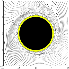
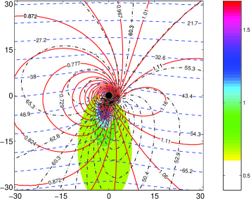
Figure 1: Describing the GR effects acting on radiation from a source near a Kerr black hole ($a=0.998$). Photons emerge from different points of the equatorial plane and proceed to a distant observer (located towards top of the figure), where they are collected in a detector. The light experiences an energy change and focusing effects which influence the observed spectrum. Time delays between photons are important for time-resolved spectroscopy. Left panel: the relativistic frame-dragging is illustrated here by plotting the points of intersection of the rays emerging from the equatorial plane. A polar grid was used, uniformly spaced in the observer plane (inclination $\theta_{\mathrm{o}}=60$ deg; $\theta_{\mathrm{o}}=90$ deg corresponds to edge-on observation, i.e. in the plain of the disc). The points of intersection form ellipses which exhibit progressive distortion near the hole. The frame-dragging is clearly visible (the hole rotates counter-clockwise; the radii of horizon and of the co-rotating innermost stable orbit are indicated by circles around the origin). Right panel: Four sets of contours are shown. They correspond to (i) redshift function (solid lines); (ii) time delay (dashed); (iii) emission angle with respect to the local normal direction (dot-dashed); and (iv) radiation flux enhancement due to gravitational lensing (different levels of shading). Knowledge of these quantities is sufficient to compute the GR effects that are expected in observed spectra. Both plots have been constructed in Boyer-Lindquist coordinates; lengths are expressed in units of $GM_{\bullet}/c^{2}$.

3 GR effects on light from accretion discs

The role of the central gravitational field is illustrated in figure 1. Here, a view of the disc plane is shown as seen from above, along the BH rotation axis (it is assumed that the disc co-rotates with the hole around their common axis). What we see is a complicated interplay of geometrical effects originating from the high curvature and rotation of the BH spacetime, and the abberation effects which result from the orbital motion of matter. All these need to be taken into account when determining the expected lightcurves (figure 2). Proceeed to the contribution by G. Matt in this volume for more details on GR effects seen in X-ray line spectra .

The geometrical optics approximation is adequate and hence the task is reduced to integration of null geodesics. Many people have tackled this problem by following Synge (1967) and assuming a fixed geometry of the spacetime. Such an approach is well substantiated because it is the black hole that is of particular interest, while the disc gravity plays only a secondary role on the spacetime metric (it may be important, however, in gamma-ray burst models in which a companion neutron star becomes tidally disrupted). This situation is useful also for purposes of illustration (the case of a heavy disc poses a mathematically and computationally more challenging task because it requires to search for a simultaneous solution of Einstein’s equations; see Karas et al. 1995; Usui et al. 1998).

The basic properties of BH X-ray spectra from the innermost regions of an accretion disc are well-known (Fabian et al. 2000; Reynolds & Nowak 2003). The so called disc–line scheme has been widely applied because it allows us to study how the spectral characteristics are formed when accretion proceeds in strong gravity (Fabian et al. 1989). The main spectral components are the X-ray continuum – primary and reflected, and the lines – notably, the iron K$\alpha$ line (a doublet with the rest energy of $\simeq 6.4$ keV) and the higher ionisation lines ($\simeq 6.7$–$6.9$ keV). The line is likely formed within a narrow interval of radii outside $r_{\rm{}ms}$ with the local intensity $I(r)$ decreasing outwards. However, the effects of the BH gravity are smeared in real observations in which the signal comes from different, insufficiently resolved regions. Because of the integration time, the mean spectrum does not distinguish an orbiting source, such as a spot, from the entire ring.

Figure 2: Typical profiles of photometric light-curves from an orbiting spot (Karas 1996). The flux has been normalized to the maximum value. Parameters of each panel: (a) $r=3$, $\theta_{\mathrm{o}}=80$ deg (lensing peak dominates the lightcurve near the orbital phase $0.5$); (b) $r=44$, $\theta_{\mathrm{o}}=80$ deg; (c) $r=44$, $\theta_{\mathrm{o}}=20$ deg (Doppler peak dominates near the phase $0.75$). Each curve has been normalized to the maximum flux. The orbital phase captures one revolution of the spot near a maximally rotating black hole.

The gravitational field is described by the metric of Kerr black hole (Misner et al. 1973):

$$ds^{2} = -\frac{\Delta}{\Sigma}\Big{(}dt-a\sin^{2}\theta\;d\phi\Big{)}^{2}+\frac{\Sigma}{\Delta}\;dr^{2}+\Sigma\;d\theta^{2}$$ (1)

$$+\frac{\sin^{2}\theta}{\Sigma}\Big{[}a\;dt-\big{(}r^{2}+a^{2}\big{)}\;d\phi\Big{]}^{2}$$

in Boyer-Lindquist spheroidal coordinates, where functions $\Delta(r)$ and $\Sigma(r,\theta)$ are known. Self-gravitation of the accreted gas is not taken into account in our discussion here. Among the properties of the metric (1) is the fact that the horizon occurs at $\Delta(r)=0$. Assuming sub-maximal rotation of the BH, $|a|\leq 1$, the outer radius is found at the dimension-less $r=1+(1-a^{2})^{1/2}$ and it hides the singularity from a distant observer. As a purely GR effect, once $a\neq 0$ all particles and photons are dragged to co-rotation with the black hole.

Neglecting the disc gravity is an entirely adequate assumption for the inner regions of AGN accretion discs (Novikov et al. 1973). However, the ‘standard’ black hole disc model does not seem to reproduce the required broadening of the iron line even if it is supplemented by a local corona above the disc. Generalized approaches have been discussed and the standard picture of the disc continuum spectrum was reconsidered to account for self-gravity (Laor & Netzer 1989). Karas et al. (1995) examined the gravitational effects the disc might have on the observed line profiles; the increase of the equivalent width was found to be only moderate.

The very existence of the innermost stable orbit is due to general relativity. For a co-rotating equatorial disc this orbit has the radius (Bardeen et al. 1972)

$$r_{\rm{}ms}=3+z_{2}-\big{[}\left(3-z_{1})(3+z_{1}+2z_{2}\right)\big{]}^{\frac{1}{2}},$$ (2)

where $z_{1}=1+\alpha_{+}\alpha_{-}[\alpha_{+}+\alpha_{-}]$, $\alpha_{\pm}=(1{\pm}a)^{\frac{1}{3}}$, and $z_{2}=(3a^{2}+Z_{1}^{2})^{\frac{1}{2}}$. The marginally stable radius spans the range from $r_{\rm{}ms}=1$ (for $a=1$, i.e. a maximally co-rotating BH) to $r_{\rm{}ms}=6$ (for $a=0$, a static BH). Black-hole rotation is limited to an equilibrium value by photon recapture from the disc (which for the standard disc model yields an equilibrium value of $a\dot{=}0.998$; Thorne 1974) and by magnetic torques (Krolik et al. 2005).

For a source of light obeying purely prograde Keplerian motion the orbital velocity is

$$v^{(\phi)}=\Delta^{-1/2}\left(r^{2}-2ar^{1/2}+{a}^{2}\right)\left(r^{3/2}+{a}\right)^{-1}.$$ (3)

Here, velocity is defined with respect to a locally non-rotating observer at the corresponding radius. The corresponding angular velocity is $\Omega(r;a)=(r^{3/2}+{a})^{-1}$, which also determines the orbital period $t_{\rm{}orb}$. In order to derive the time and frequency measured by a distant observer, one needs to take into account the Lorentz factor associated with the orbital motion,

$$\Gamma=\frac{\left(r^{3/2}+{a}\right)\Delta^{1/2}}{r^{1/4}\;\sqrt{r^{3/2}-3r^{1/2}+2{a}}\;\sqrt{r^{3}+{a}^{2}r+2{a}^{2}}}\,.$$ (4)

By ignoring all other sources of gravitation except the central black hole we assume there are no secondary bodies influencing gravitationally the inner disc. (This may not be true in case of binary BHs or in the presence of global magnetic fields that can warp the disc away from a unique plane.) The radiation field is then determined by solving Maxwell’s equations for the electromagnetic field tensor and its dual in a fixed curved spacetime. In the vacuum we write: ${F^{\mu\nu}}_{\!;\nu}=0$, and ${{}^{\star}F^{\mu\nu}}_{\!;\nu}=0$, where the asterisk denotes a dual tensor. Electric field components can be obtained by projection onto observer’s four-velocity, $E^{\alpha}=F^{\alpha\beta}u_{\beta}$, and an electromagnetic wave is defined as an approximate test-field solution of the form

$$F_{\alpha\beta}=\Re e\left[u_{\alpha\beta}\;e^{\Im\psi(x)}\right].$$ (5)

Two scales are introduced at this point. The phase $\psi(x)$ is assumed to be a rapidly varying function, while the amplitudes $u_{\alpha\beta}$ vary slowly. This allows us to define a wave vector, $k_{\alpha}\equiv\psi_{,\alpha}$, which is parallelly transported along the null geodesics, $k_{\alpha;\beta}\,k^{\beta}=0$, $k_{\alpha}k^{\alpha}=0$. The propagation law in the empty space is (Anile & Breuer 1974)

$$DF_{\alpha\beta}-2\theta F_{\alpha\beta}=0,$$ (6)

where $\theta\equiv-\frac{1}{2}{k^{\alpha}}_{;\alpha}$ describes the expansion of null congruences, $D\,\equiv\,u^{\alpha}\nabla_{\alpha}$.

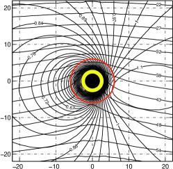
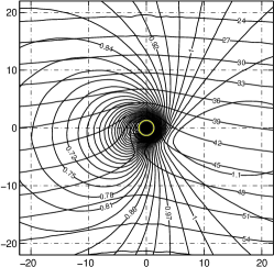
Figure 3: Isocontours of constant light-travel time $\delta{t}$ (approximately horizontal lines) and of the redshift function $1+z$ (loops) are shown in the equatorial plane of the Kerr BH. Two panels are shown for a non-rotating BH ($a=0$, left), and for a maximally rotating BH ($a=1$, right). For $a=0$, three circles are plotted with radii of the horizon, the circular photon orbit, and the marginally stable orbit. The three radii appear to coincide with each other in the maximally rotating case (co-rotating orbits are assumed). In the plunging region (shaded) the form of the isocontours depends on the assumed motion of the material, which no longer maintains Keplerian $r=\mbox{const}$ orbits; magnetic fields likely play a major role here. All values are given in geometrized units, observer’s inclination is $\theta_{\mathrm{o}}=50$ deg.

Having in mind the applications to present-day X-ray observations, the energy shifts, gravitational lensing and time delays are the principal effects which originate from general relativity and can be tested with data that are in our disposal. Polarimetric information goes beyond this limit and has a capability of constraining parameters of our models at a higher level. Different approaches to polarimetry and specific issues of X-ray polarimetry were discussed by various authors, namely, Cocke & Holm (1972), Anile et al. (1974, 1977), Madore (1974), Bičák & Hadrava (1975). In strong gravity, the covariant definition of basic polarimetric quantities is appropriate and it was developed in various flavours: see Breuer & Ehlers (1980) and Anile (1989) for the definition of the polarization tensor, $J_{\alpha\beta\gamma\delta}\,\equiv\,\frac{1}{2}\langle F_{\alpha\beta}F_{\gamma\delta}\rangle$. A recent discussion was given in Broderick & Blandford (2003).

At first, projections $J_{\alpha\beta}=J_{\alpha\beta\gamma\delta}\,u^{\gamma}\,u^{\delta}=\langle E_{\alpha}\bar{E}_{\beta}\rangle$ are introduced. Four parameters $S_{A}$ are then given by $S_{\!{}_{A}}\equiv\frac{1}{2}(k_{\alpha}u^{\alpha})^{2}F_{\!{}_{A}}$, where $F_{\!{}_{A}}$ $(A=0,\,\ldots\,3)$ are again constructed by projecting the polarization tensor (Anile & Breuer 1974). These quantities satisfy the relations $J_{\alpha\beta}u^{\beta}=0$, $J_{\alpha\beta}k^{\beta}=0$, $\omega=u_{\alpha}k^{\alpha}$ and can be connected with the traditional definition of the Stokes parameters (Stokes 1852; Chandrasekhar 1960).

The normalized Stokes parameters are $s_{1}\,\equiv\,S_{1}/S_{0}$, $s_{2}\,\equiv\,S_{2}/S_{0}$, and $s_{3}\,\equiv\,S_{3}/S_{0}$. The degree of linear and of circular polarization is $\Pi_{l}=\sqrt{s_{1}^{2}+s_{2}^{2}}$, $\Pi_{c}=|s_{3}|$, and the total degree of polarization $\Pi=\sqrt{\Pi_{l}^{2}+\Pi_{c}^{2}}$.

Upon propagation through an arbitrary (curved but empty) space-time, the radiation flux obeys the well-known relation, $F_{\!{}_{A,\,\rm em}}\,dS_{{}_{\rm em}}=F_{\!{}_{A,\,\rm obs}}\,dS_{{}_{\rm obs}}$ from which one can relate the redshift $z$ at the point of emission with the redshift at a distant observer,

$$1+z=\frac{(k_{\alpha}u_{\alpha})_{\rm em}}{(k_{\alpha}u_{\alpha})_{\rm obs}},\quad S_{\!{}_{A}}=\frac{k_{\!{}_{A}}}{(1+z)^{2}dS}.$$ (7)

In the Kerr metric–thin disc case, the redshift factor $z$ and the local emission angle $\vartheta$ are given by

$$1+z=\frac{r^{3/2}-3r^{1/2}+2a}{r^{3/2}+{a}-\xi},\quad\cos\vartheta=\frac{g\eta^{1/2}}{r};$$ (8)

$\xi$ and $\eta$ are constants of motion (they are connected with the photon ray and exist in every axially symmetric and stationary spacetime; see figure 3). Let us remark that generalizations to non-Keplerian motion of the reflecting material were discussed by several authors: Reynolds & Begelman (1997) discussed radiation from the plunging region with matter in free-fall motion, and Dovčiak et al. (2004) implemented this possibility in the ky code. Also Fukue (2004) examined the non-negligible radial component of velocity.

To explore GR effects from BH accretion discs, ky is currently the most versatile code available publicly and included in the spectral fitting xspec package. It allows its user to specify time-dependent/non-axisymmetric emissivity $I(t;r,\phi)$ of the disc (e.g. spiral waves), explore the plunging region (e.g. falling blobs), and to vary the black-hole angular momentum as well as the inner edge of the disc as free parameters. The code has also capacity to study GR polarization; this option cannot be currently exploited in practice and we need to wait for future satellites to perform the job. However, it is interesting to note that a complementary task can be partially accomplished with the help of ground based near-infrared observations of the Galaxy Center flares (see also Hollywood & Melia 1997). Future X-ray satellite data will be essential to study GR in the neighbourhood of accreting black holes with outstanding precision.

Figure 4: Radius $r$ at which the maximum energy shift, $g_{+}(r)_{|r=\mbox{const}}$, reaches its peak value as a function of the inclination $\theta_{\mathrm{o}}$. This shows how large excursions of the blue peak of the line can be expected. For $\theta_{\mathrm{o}}>60$ deg the maximum occurs at the marginally stable orbit where the inner edge of the disc is often assumed (details in Pecháček et al. 2005). More complete information about the observed width of the line can be obtained from graphs of the redshift factor and the gravitational lensing, as they vary across the disc surface (see the paper by Matt in this volume).

In a typical situation of an AGN accretion disc, and especially for small radii and intermediate to large inclination angles, the line emission comes from a small fraction of the orbit. This implies that for observations with a moderate signal-to-noise ratios, only a narrow blue horn is expected to appear for brief time. Figure 4 shows how large variations of the line energy arise at different parts of the orbit.

Eq. (7) shows that the polarization properties of the disc emission are modified by the photon propagation in the gravitational field and they may provide additional information about the field structure. Since the reflecting medium has a disc-like geometry, a substantial amount of linear polarization is expected because of Compton scattering. The set of four Stokes parameters describes polarization properties of the scattered light entirely. However, in order to compute the observable characteristics, i.e. count rates of different polarization modes, one has to combine the reflected component with the primary continuum. The polarization degree of the resulting signal depends on the mutual proportion of the two components.

The idea of using polarimetry to gain additional information about compact objects is not a new one. In this context it was proposed by Rees (1975) that polarized X-rays are of high relevance. Pozdnyakov et al. (1979) studied spectral profiles of X-ray iron lines that result from multiple Compton scattering (also Angel 1969; Bonometto et al. 1970; Sunyaev & Titarchuk 1985; Matt 1993). The possibility of detecting gravitational effects on polarized X-rays is very attractive as it has great potential in revealing black holes, but the idea still awaits precise formulation as well as the technology usable for its practical implementation. Temporal variations of polarization were discussed, in particular the case of orbiting spots (Pineault 1977; Connors et al. 1980; Bao et al. 1998). Further aspects of GR were examined by Viironen & Poutanen (2004), Dovčiak et al. (2004a), and Horák & Karas (2006a, b), who studied the role of multiple images.

4 Spots and spirals

In their seminal papers, Cunningham & Bardeen (1972, 1973) studied the radiation from a star revolving in the equatorial plane of a maximally rotating BH. They presented a detailed analysis of periodic variations of the observed frequency-integrated flux that arrives at the observer. The method turns out to be a very practical one, even three decades later when computer capabilities have increased tremendously. However, the potential of their idea cannot be fully exploited until the theory determines the intrinsic emission that emerges locally from the disc. Neither it is well-suited for timing analyses (current status of this effort is summarized by Goosmann in this volume).

Since first attempts, which were largely limited to photometry, many people have developed various modifications of the original semi-analytical approach, especially for the spectroscopy of accretion discs: Cunningham (1975); Gerbal & Pelat (1981); Asaoka (1989); Bao & Stuchlík (1989); Viergutz (1993); Rauch & Blandford (1994); Zakharov (1994); Bromley et al. (1997); Fanton et al. (1997); Bao et al. (1998); Semerák et al. (1999); Martocchia et al. (2000); Schnittman (2005), and others. Computational challenges have been largely overcome thanks to a combination of semi-analytical approaches and sophisticated numerical algorithms. The analytical part of the work is largely based on the remarkable property of the geodesic motion in Kerr metric (due to Carter 1968), which is integrable and can be carried out in terms of elliptical integrals (de Felice et al. 1974; Sharp 1979; Čadež & Calvani 2005). The numerical approach often employs pre-computed data that are stored for the subsequent light-ray reconstruction (Karas et al. 1992; Dovčiak et al. 2004b; Beckwith & Done 2004). Whichever strategy is adopted, the ray-tracing core of the code has to be connected with a radiation transfer routine determining the intrinsic spectrum and, indeed, the understanding of the transfer problem has been tremendously improved in recent years.

The idea of magnetic flares irradiating the disc surface (Merloni & Fabian 2001) gives a promising route towards a more complete physical formulation of the ‘bright-spot’ model that would be based on elementary processes and help reducing the excessive number of degrees of freedom. By employing this approach, Czerny et al. (2004) computed the reprocessed spectra and compared the predicted variability with MCG–6-30-15 observational data. The actual size of the spot is linked with the X-ray flux which originates in flares and depends on the vertical height where the flares occur above the disc plane. The induced rms variability is a function of the energy range of the observation and the model parameters including the BH angular momentum and the position of the disc inner edge. Goosmann et al. (2006) examined different cases with the spot size and height ranging from a fraction of $r_{\rm{}g}$ to several $r_{\rm{}g}$. It is interesting to notice that the lamp-post geometry is a limiting case of the flare/spot model. These results can reproduce the observed features, albeit the present data do not constrain all parameters; for example the spot size cannot be determined.

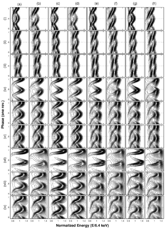
Figure 5: An examplary set of dynamical spectra of a two-arm spiral pattern with a slowly decaying flare. Different cases correspond to the form of the spiral, rotation parameter of the BH, and observer’s viewing angle. These translate to different amplitudes and energy ranges spanned by observed spectra. The model parameters can be assorted in four categories: (A) BH angular momentum: $a=0$ (columns denoted by letters a, c, e, g), and $a=1$ (b, d, f, h). (B) Observer inclination: $\theta_{\mathrm{o}}=20$ deg (the rows denoted by roman numbers i–iii), $\theta_{\mathrm{o}}=50$ deg (iv–vi), and $\theta_{\mathrm{o}}=80$ deg (vii–ix). (C) The extent of the spiral; here, the outer edge is located at: $r_{0}=7$ (i, iv, vii), $r_{0}=13$ (ii, v, viii), and $r_{0}=20$ (iii, vi, ix). (D) The actual form of the spiral structure is defined by the pitch angle $\arctan\alpha$ and the contrast from the background $\beta$: $\alpha=3$, $\beta=8$ (a, b); $\alpha=\sqrt{3}$, $\beta=8$ (c, d); $\alpha=6$, $\beta=8$ (e, f); $\alpha=6$, $\beta=18$ (g, h). For details see Karas et al. (2001).

A complementary picture assumes extended and evolving shapes of the reflection area on the disc. Spiral shapes can arise from an extended spot following its decay by shearing motion under various kinds of instabilities operating in the disc. Such patterns are transient but may last over a substantial fraction of the orbital period, sufficiently long to produce observable effects. Apart from AGN discs they have been invoked also to explain the flares in Sagittarius A^⋆ (Tagger & Melia 2006) for which individual clumps rather than a continuous accretion flow seem to be responsible. Examples and useful templates of the expected spectral line profiles were computed (Chakrabarti & Wiita 1993; Karas et al. 2001; Hartnoll & Blackman 2002; Fukumura & Tsuruta 2004); see figure 5 where a combination of an instantaneous flare and a persisting spiral was assumed. Here, the flare quickly perishes and the spiral dominates the spectrum. The spiral is described by its pitch angle $\arctan\alpha$ (tightly wound spirals are described by large values of the pitch angle) and the contrast $\beta$ (well-defined patterns have a large $\beta$). On the inner side the spiral terminates at $r=r_{\rm{}ms}$. In each panel the spectra were computed in $10^{2}\times 10^{2}$ energy–phase grid by our Kerr metric ray-tracing code.

5 Conclusions

The influence of strong gravity on light provides a possibility to study black holes. However, gravity is not the only agent that shapes the observed spectra; emission mechanisms and radiation transfer in the accreting gas need to be understood reliably. Remarkable progress has been achieved on the way to model the physical processes which govern the form of X-ray reflection spectra emerging from different regions of accretion discs. In spite of this advance the current description still contains some elements of the phenomenological approach and the emission from non-axisymmetric patterns cannot be computed entirely ‘from first principles’. Nonetheless, already at its present formulation the model of a spotted disc helps us to constrain the parameters of accreting black holes. The orbital radius of the peak emission and the disc inclination can be inferred from the variations of the observed line width and the centroid energy. $M_{\bullet}$ can be estimated by comparing the measured orbital period with the value expected for the derived radius. The model of spirals also gives the possibility of tracing the surface structures on accretion discs. Once these are determined the goal of measuring black hole rotation will be feasible with unprecedented accuracy.

- [1] Abramowicz M. A., Bao G., Lanza A., Zhang X.-H.: 1991, A&A 245, 454
- [2] Abramowicz M. A., Lanza A., Spiegel E. A., Szuszkiewicz E.: 1992, Nature, 356, 41
- [3] Adams F. C., Watkins R.: 1995, ApJ, 451, 314
- [4] Angel J. R. P.: 1969, MNRAS, 158, 219
- [5] Anile A. M.: 1989, Relativistic fluids and magneto-fluids (Cambridge: Cambridge University Press)
- [6] Anile A. M., Breuer R. A: 1974, ApJ, 189, 39
- [7] Anile A. M., Pantano P.: 1977, Phys. Lett. A, 61, 215
- [8] Antonicci A., Gómez de Castro A. I.: 2005, A&A, 432, 443
- [9] Asaoka I.: 1989, PASJ, 41, 763
- [10] Ballantyne D. R., Fabian A. C.: 2003, ApJ, 592, 1089
- [11] Ballantyne D. R., Ross R. R., Fabian A. C.: 2001, MNRAS, 327, 10
- [12] Bao G., Stuchlík Z. 1992, ApJ, 400, 163
- [13] Bao G., Wiita P. J., Hadrava P.: 1998, ApJ, 504, 58
- [14] Bardeen J. M., Press W. H., Teukolsky S. A.: 1972, ApJ, 178, 347
- [15] Beckwith K., Done C.: 2004, MNRAS, 353, 362
- [16] Bičák J., Hadrava P.: 1975, A&A, 44, 389
- [17] Blandford R. D., McKee C. F.: 1982, ApJ 255, 419
- [18] Bonometto S., Cazzola P., Saggion A.: 1970, A&A, 7, 292
- [19] Brenneman L. W., Reynolds C. S.: 2006, ApJ, in press
- [20] Breuer R. A., Ehlers J.: 1980, Proc. Roy. Soc. Lond. A, 370, 389
- [21] Broderick A. E., Blandford R. D.: 2003, MNRAS, 342, 1280
- [22] Bromley B. C., Chen K., Miller W. A.: 1997, ApJ, 475, 57
- [23] Čadež A., Calvani M.: 2005, MNRAS, 363, 177
- [24] Carter B.: 1968, Physical Review, 174, 1559
- [25] Chakrabarti S. K., Wiita P. J.: 1993, A&A, 271, 216
- [26] Chandrasekhar S.: 1960, Radiative Transfer (New York: Dover)
- [27] Cocke W. J., Holm D. A.: 1972, Nature Physical Science, 240, 161
- [28] Collin S., Dumont A.-M., Godet O.: 2004, A&A, 419, 877
- [29] Connors P. A., Stark R. F., Piran T.: 1980, ApJ, 235, 224
- [30] Cunningham C. T.: 1975, ApJ, 202, 788
- [31] Cunningham C. T., Baardeen J. M.: 1972, ApJ, 173, L137
- [32] Cunningham C. T., Baardeen J. M.: 1973, ApJ, 183, 273
- [33] Czerny B., Różańska A., Dovčiak M., Karas V., & Dumont A.-M.: 2004, A&A, 420, 1
- [34] de Felice F., Nobili L., Calvani M.: 1974, A&A, 30, 111
- [35] Done C., Nayakshin S.: 2001, MNRAS, 328, 616
- [36] Dovčiak M., Karas V., Matt G.: 2004a, MNRAS, 355, 1005
- [37] Dovčiak M., Karas V., Yaqoob T.: 2004b, ApJSS, 153, 205
- [38] Fabian A. C., Iwasawa K., Reynolds C. S., Young A. J.: 2000, PASP, 112, 1145
- [39] Fabian A. C., Rees M. J., Stella L., White N. E: 1989, MNRAS, 238, 729
- [40] Fanton C., Calvani M., de Felice F., Čadež A.: 1997, PASJ, 49, 159
- [41] Fukue J.: 1987: Nature, 327, 600
- [42] Fukue J.: 2004, Progress of Theor. Phys. Suppl., 155, 329
- [43] Fukumura K, Tsuruta S.: 2004, ApJ, 613, 700
- [44] Galeev A. A., Rosner R., Vaiana G. S.: 1979, ApJ, 229, 318
- [45] Gerbal D., Pelat D.: 1981, A&A, 95, 18
- [46] Goosmann R., Czerny B., Mouchet M., Ponti G., Dovčiak M., Karas V., Różańska A., Dumont A.-M.: 2006, A&A, 454, 741
- [47] Hartnoll S. A., Blackman E. G.: 2000, MNRAS, 317, 880
- [48] Hartnoll S. A., Blackman E. G.: 2002, MNRAS, 332, L1
- [49] Henri G., Pelletier G.: 1991, ApJ, 383, L7
- [50] Hollywood J. M., Melia F.: 1997, ApJSS, 112, 423
- [51] Horák J., Karas V., 2006a, MNRAS, 365, 813
- [52] Horák J., Karas V., 2006b, PASJ, 58, 203
- [53] Kallman T. R., Palmeri P., Bautista M. A., Mendoza C., Krolik J. H.: 2004, ApJSS, 155, 675
- [54] Karas V.: 1996, ApJ, 470, 743
- [55] Karas V.: 1997, MNRAS, 288, 12
- [56] Karas V., Czerny B., Abbrasart A., Abramowicz M. A.: 2000, MNRAS, 318, 547
- [57] Karas V., Bao G.: 1992, A&A, 257, 531
- [58] Karas V., Lanza A., Vokrouhlický D.: 1995, ApJ, 440, 108
- [59] Karas V., Martocchia A., Šubr L.: 2001, PASJ, 53, 189
- [60] Karas V., Vokrouhlický, Polnarev A. G.: 1992, MNRAS, 259, 569
- [61] Kawaguchi T., Mineshige S., Machida M., Matsumoto R., Shibata K.: 2000, PASJ, 52, L1
- [62] Krolik J. H.: 1999, Active Galactic Nuclei (Princeton: Princeton University Press)
- [63] Krolik J. H., Hawley J. F., Hirose S.: 2005, ApJ, 622, 1008
- [64] Laor A.: 1991, ApJ, 376, 90
- [65] Laor A., Netzer H.: 1989, MNRAS, 238, 897
- [66] Lawrence A., Papadakis I.: 1993, ApJ, 414, 85
- [67] Madore J.: 1974, Comm. Math. Phys., 38, 103
- [68] Mangalam A. V., Wiita P. J.: 1993, ApJ, 406, 420
- [69] Martocchia A., Karas V., Matt G.: 2000, MNRAS, 312, 817
- [70] Martocchia A., Matt G.: 1996, MNRAS, 282, 53
- [71] Matt G.: 1993, MNRAS, 260, 663
- [72] Matt G., Perola G. C.: 1992, MNRAS, 259, 433
- [73] Merloni A., Fabian A. C.: 2001, MNRAS, 328, 958
- [74] Misner C. W., Thorne K. S., Wheeler J. A.: 1973, Gravitation (San Francisco: Freeman)
- [75] Nayakshin S., Kazanas D., Kallman T. R.: 2000, ApJ, 537, 833
- [76] Novikov I. D., Thorne K. S.: 1973, in Black Hole Astrophysics, C. DeWitt and B. S. DeWitt (eds), (New York: Gordon & Breach), p. 343
- [77] Pecháček T., Dovčiak M., Karas V., Matt G.: 2005, A&A, 441, 855
- [78] Peterson B. M.: 1997, Active Galactic Nuclei (Cambridge: Cambridge University Press)
- [79] Pineault S.: 1977, MNRAS, 179, 691
- [80] Poutanen J., Fabian A. C.: 1999, MNRAS, 306, 31
- [81] Pozdnyakov L. A., Sobol I. M., Sunyaev R. A.; 1979, A&A, 75, 214
- [82] Rauch K. P., Blandford R. D.: 1994, ApJ, 421, 46
- [83] Rees M. J.: 1975, MNRAS, 171, 457
- [84] Reynolds C. S., Begelman M. C.: 1997, ApJ, 488, 109
- [85] Reynolds C. S., Nowak M. A.: 2003, Phys. Rep., 377, 389
- [86] Ross R. R., Fabian A. C.: 2005, MNRAS, 358, 211
- [87] Różańska A., Dumont A.-M., Czerny B., Collin S.: 2002, MNRAS, 332, 799
- [88] Sanbuichi K., Fukue J., Kojima Y.: 1994, PASJ, 46, 605
- [89] Schnittman J. D.: 2005, ApJ, 621, 940
- [90] Semerák O., Karas V., de Felice F.: 1999, PASJ, 51, 571
- [91] Shaffee R., McClintock J. E., Narayan R., Davis S. W., Li Li-Xin, Remillard R. A.: 2006, ApJ, 636, L113
- [92] Sharp N. A.: 1979, Gen. Rel. Grav., 10, 659
- [93] Stella L.: 1990, Nature, 344, 747
- [94] Stokes G.: 1852, Trans. Cambridge Phil. Soc., 9, 399
- [95] Sunyaev R. A., Titarchuk L. G.: 1985, A&A, 143, 374
- [96] Synge J. L.: 1967, MNRAS, 136, 195
- [97] Tagger M., Henriksen R. N., Sygnet J. F., Pellat R.: 1990, ApJ, 353, 654
- [98] Tagger M., Melia F.: 2006, ApJ, 636, L33
- [99] Taylor J. A.: 1996, ApJ, 470, 269
- [100] Thorne K. S.: 1974, ApJ, 191, 507
- [101] Turner T. J., Mushotzky R. F., Yaqoob T., George I. M., Snowden S. L., Netzer H. et al.: 2004, ApJ, 574, L123
- [102] Usui F., Nishida S., Eriguchi Y.: 1998, MNRAS, 301, 721
- [103] Viergutz S. U.: 1993, A&A, 272, 355
- [104] Viironen K., Poutanen J.: 2004, A&A, 426, 985
- [105] Zakharov A. F.: 1994, MNRAS, 269, 283
- [106] Życki P. T.: 2002, MNRAS, 333, 800