Buoyant magnetic flux ropes in a magnetized stellar envelope

Abstract

Context. The context of this paper is buoyant toroidal magnetic flux ropes, which is a part of flux tube dynamo theory and the framework of solar-like magnetic activity.

Aims. The aim is to investigate how twisted magnetic flux ropes interact with a simple magnetized stellar model envelope—a magnetic “convection zone”—especially to examine how the twisted magnetic field component of a flux rope interacts with a poloidal magnetic field in the convection zone.

Methods. Both the flux ropes and the atmosphere are modelled as idealized 2.5-dimensional concepts using high resolution numerical magneto-hydrodynamic (MHD) simulations.

Results. It is illustrated that twisted toroidal magnetic flux ropes can interact with a poloidal magnetic field in the atmosphere to cause a change in both the buoyant rise dynamics and the flux rope’s geometrical shape. The details of these changes depend primarily on the polarity and strength of the atmospheric field relative to the field strength of the flux rope. It is suggested that the effects could be verified observationally.

1 Introduction

Buoyant magnetic flux tubes are an essential part of the framework of current theories of dynamo action in both the Sun and solar-like stars: it is widely believed that flux tubes are formed by some combination of rotational shear and turbulent convection near the bottom of the convection zones (CZ) of these stars. When sufficiently buoyant the magnetic flux rise in the form of tubular (toroidal) $\Omega$-shaped loops of magnetic field lines. Rising under the influence of rotational forces, the loops finally emerge as slightly asymmetric and tilted bipolar magnetic regions at the surface, see e.g. Fan et al. (1994) and Caligari et al. (1995). During the last decade, it has been established that if they do exist, these flux tubes must in fact be flux ropes of intertwined or twisted field lines; otherwise they would quickly be disrupted by a magnetic “mushrooming” instability, see e.g. Emonet & Moreno-Insertis (1998) and Dorch & Nordlund (1998). It has been shown that the instability is inhibited if the degree of systematic twist is sufficiently high, corresponding to a critical value of the field line pitch angle $\Psi_{c}$ approximately determined by equality between the energy density of the twisted field component and the ram pressure due to the rise of the flux rope e.g. Moreno-Insertis & Emonet (1996).

A fundamental ingredient in all theories of solar-like dynamos is a process where a relatively weak poloidal magnetic field is turned into a toroidal field by differential rotation: it is this toroidal field that eventually gives rise to the flux ropes, which at the end of their existence return a poloidal field component to the CZ, thereby completing the magnetic activity cycle. This dynamo process is gradual and different cycles overlap.

Buoyant magnetic flux ropes have been extensively study through numerical simulations, cf. the reviews in Dorch (2002) and Fan (2004), and the most recent high resolution study in two dimensions by Cheung et al. (2006). However, so far studies of the interaction of flux ropes with poloidal fields have solely dealt with flux ropes that emerge into the solar corona, e.g. Archontis et al. (2004), i.e. not with a magnetic CZ.

The question addressed in this paper is how the polarity and strength of the field in a magnetized convection zone may affect the rise and evolution of twisted flux ropes. When the predominantly toroidal buoyant flux ropes rise through the CZ, they encounter a poloidal magnetic field that has a component perpendicular to the ropes’ axes. However, since the flux ropes are twisted, the transversal field components may be either parallel or anti-parallel to the average magnetic field in the CZ, i.e. the field in the two-dimensional plane perpendicular their toroidal axis.

Several questions relevant to the theory of flux tube dynamos then emerge: e.g. is the rise faster or slower and do more or less magnetic flux reach the surface in the presence of a magnetized convection zone; how does a magnetized convection zone affect the required amount of twist. In this paper I attempt to shed light on these questions by presenting results from idealized numerical 2.5-dimensional MHD simulations of the cross-sections of buoyant flux ropes that interact with a horizontal magnetic layer while they rise.

2 Model

The full compressible MHD-equations are solved using the stagger-code by Galsgaard and others, cf. Galsgaard & Nordlund (1997):

$${\frac{\partial{\bf\rho}}{\partial t}} = -\nabla\cdot\rho{\bf u},$$ (1)

$${\frac{\partial{({\rho}{\bf u})}}{\partial t}} = -\nabla P+{\bf j}\times{\bf B}-\nabla\cdot(\rho{\bf u}{\bf u})+\nu\nabla^{2}\rho{\bf u},$$ (2)

$${\frac{\partial e}{\partial t}} = -\nabla\cdot(e{\bf u})-P\nabla\cdot{\bf u}+Q_{\rm v}+Q_{\rm J},$$ (3)

$$\frac{\partial{\bf B}}{\partial t} = \nabla\times({\bf u}\times{\bf B})+\eta\nabla^{2}{\bf B},$$ (4)

Here $\rho$ is the fluid density, ${\bf u}$ is the velocity, $P$ the gas pressure, ${\bf j}$ is the electric current density, ${\bf B}$ is the magnetic field density and $e$ is the internal energy. In Eq. (2) ${\bf j}\times{\bf B}$ is the Lorentz force and $Q_{{\rm v}}$ and $Q_{{\rm J}}$ are the viscous and Joule dissipation respectively.

The equations are solved numerically on a staggered mesh using derivatives and interpolations that are of 6th and 5th order respectively in a numerical scheme that conserves $\nabla\cdot{\bf B}=0$ exactly. The time stepping is implemented by a third order predictor-corrector method. Numerical solutions are obtained on a high-resolution two-dimensional Cartesian grid of $2048^{2}$ points. The initial set-ups of the models are twofold, consisting of a snapshot of a stratified and magnetized adiabatic CZ-model, and of an idealized twisted magnetic flux rope.

Initially the entropy in the interior of the ropes are set equal to that in the external medium leading to a buoyancy equal to $1/\gamma\beta$ (with $\gamma=5/3$). The coordinate system is chosen such that $x$ is the vertical coordinate, $y$ the horizontal coordinate and $z$ is the coordinate along the axis which is parallel to the rope.

The flux ropes move in a polytropic atmosphere $P=P_{0}(\rho/\rho_{0})^{\gamma}$, where $P_{0}$ and $\rho_{0}$ are the quantities at the initial position of the flux rope corresponding to a pressure scale height of ${\rm H}_{\rm P0}=59$ Mm. The top pressure scale height is one tenth of the bottom scale height ${\rm H}_{\rm P0}$. The upper boundary is well below the position of an imagined photosphere. Horizontally the boundaries are periodic and the physical size of the computational box is 136 Mm in both the vertical and horizontal dimensions corresponding to a height of 2.3 ${\rm H}_{\rm P0}$. The initial position of the flux ropes are set to $x=0.27\leavevmode\nobreak\ {\rm H}_{\rm P0}$.

The initial twist of the flux ropes are given by

$${\rm B}_{z} = {\rm B}_{\rm 0}e^{-(r/R)^{2}}$$ (5)

$${\rm B}_{\phi} = \alpha(r/R)^{3}\leavevmode\nobreak\ {\rm B}_{z}e^{-(r/R)^{2}},$$ (6)

where ${\rm B}_{z}$ is the parallel (axial) and ${\rm B}_{\phi}$ the transversal component of the magnetic field with respect to the ropes’ main axes. ${\rm B}_{\rm 0}$ is the amplitude of the field, $R$ the radius, and $\alpha$ is a field line pitch parameter. The critical pitch of a twisted flux rope needed to prevent the disrupting instability depends on the ratio of the rope’s radius to the local pressure scale height: for thin flux ropes this ratio is small and in the case of the thin flux ropes studied by Emonet & Moreno-Insertis (1998), the critical pitch angle was $10^{\rm o}$. In the following I set the initial radius to $R_{0}=0.14\leavevmode\nobreak\ {\rm H}_{\rm P0}$, i.e. the tubes are non-thin yielding a critical angle of $\Phi_{c}\approx 25^{\rm o}$ according to the expression by Moreno-Insertis & Emonet (1996). To be on the safe side, $\alpha=1.75$ is chosen, so that the initial maximum field line pitch angle is $35.6^{\rm o}$, occurring at the border of the rope at $r=\sqrt{3/2}\leavevmode\nobreak\ R$ for the topology given in Eq. (6). Incidentally this is low enough that a three-dimensional flux rope would not be kink unstable, since to achieve a substantial growth rate this requires a pitch exceeding $45^{\rm o}$, e.g. Galsgaard & Nordlund (1997).

Table 1: List of numerical simulations and their basic parameters: model name, ratio of CZ field to the rope’s twisted field component $\epsilon$, sign of the latter ratio, and ratio of the rope’s axial field to the CZ field strength $\chi$ (only the value of $B_{\rm CZ}$ vary). The horizontal dividing line indicates the approximate position of the lower solar limit, i.e. $\chi_{\odot}\sim 10$.

Model	$\epsilon$	$||$	$\chi$
0	0	N/A	N/A
1A	0.044	-	90
1B	0.044	+	90
2A	0.22	-	18
2B	0.22	+	18
3A	0.44	-	9
3B	0.44	+	9
4A	2.2	-	1.8
4B	2.2	+	1.8

With a grid of 2048 points in each dimension, the flux ropes are resolved by more than 200 grid points while the resolution of the pressure scale height ${\rm H}_{\rm P0}$ is closer to 1000 grid points. From a computational point of view one has to set the ropes’ plasma $\beta$’s lower than the solar values ($10^{4}$—$10^{7}$) to reduce the computational time scale to a reasonable value: $\beta_{0}=107$ is chosen for the initial strength of the buoyancy on the ropes’ axes.

The magnetic layer is implemented by adding a magnetic field of $B_{y}=B_{\rm CZ}$ to the hydrostatic equilibrium at heights $x\geq 0.9\leavevmode\nobreak\ {\rm H}_{\rm P0}$ above the bottom of the computational box. Numerically this results in a steep gradient at that height (see the discussion on diffusion in Section 4).

For convenience I furthermore define $\chi\equiv B_{\rm rope}/B_{\rm CZ}$ for the ratio of the ropes’ axial fields to the CZ field strength, and $\epsilon\equiv B_{\rm CZ}/B_{\phi}$ for the ratio of CZ field to a characteristic value of the ropes’ twisted field components, e.g. its maximum value. In the simulations presented here both $\epsilon$ and $\chi$ are varied by a factor of 50 between the weakest and strongest CZ field strength. For all models $\epsilon\chi$ has the same value $\approx 4$. An estimated value of $\chi$ for the Sun is given by the ratio of the canonical toroidal field strength of 100 kG, to a poloidal field of at most equipartition $B_{\rm eq}\sim 10$ kG, i.e. $\chi_{\odot}\geq 10$.

It is trivial to calculate a simple limit for the strength of the envelope field $B_{\rm CZ}$ relative to the strength of rope by assuming a force balance between the buoyancy of the flux rope and the oppositely directed tension caused by a dent of magnitude $R$ in field lines in the CZ field layer: with an initial buoyancy of $1/\gamma\beta$ the order of magnitude of $\chi$ should exceed

$$\chi_{\rm c}\equiv\sqrt{\gamma\frac{2\leavevmode\nobreak\ {\rm H}_{\rm P0}}{{\rm R}}},$$ (7)

if buoyancy is to overcome the magnetic tension from the field lines in the layer. The size of the ropes in this model results in $\chi_{0}\sim 5$. For the Sun, the approximate lower bound fulfills $\chi_{\odot}>\chi_{\rm c}$ and hence solar flux ropes are expected to be able to rise through the poloidal field layer as assumed by the flux tube dynamo.

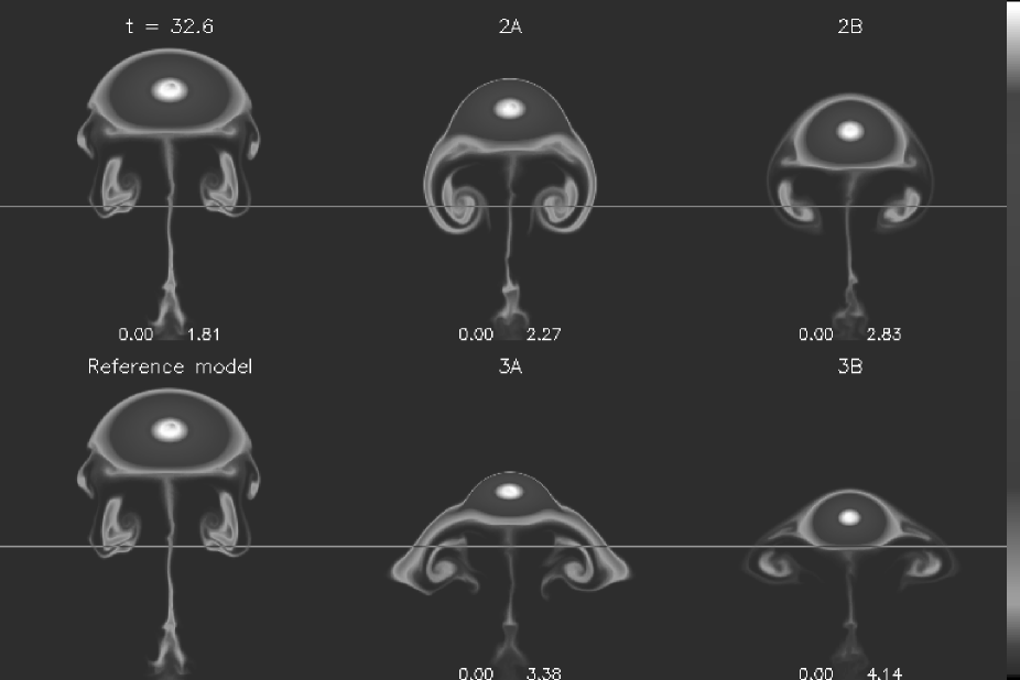
Figure 1: Grey-scale panel showing snapshots of $B_{z}$ at $t\sim 32.6$ time units for models with moderately magnetized envelopes. Minimum (zero) and maximum magnetic field strengths are stated for every snapshot (in units of 354 kG). Vertical dimension corresponds to $x$ in the simulations. Shown are model 0 (shown twice), and in the upper row models 2A and 2B (initial $B_{\rm CZ}/B_{\phi}=18$) and in the lower row models 3A and 3B (initial $B_{\rm CZ}/B_{\phi}=9$). Also shown are horizontal lines indicating the initial position of the magnetized layer.

3 Results

Several models were run, varying parameters such as numerical resolution and $B_{\rm CZ}$, but not the ropes’ initial field strengths. Table 1 lists the models that are discussed in this paper. Except from models 4A and 4B all models have $\chi>\chi_{\rm c}$.

The nine models consist of eight models of flux ropes rising into a magnetized layer corresponding to a poloidal field in a CZ and a single reference model where no CZ field was present model 0.

3.1 Flux conservation and numerical dissipation

With a weak or absent envelope magnetic field, the total magnetic flux through the plane perpendicular to a rope’s axis $\Phi_{\rm z}$ remains constant: it only decreases by 0.1 promille during the simulation runs and hence there is virtually no flux loss due to (unwanted) numerical dissipation. The total magnetic flux through the horizontal boundaries is another matter: the total flux $\Phi_{\rm y}$ through the horizontal boundary decreases constantly by typically 0.5 promille per time unit, leading to a loss of 1–3% during an entire run. This loss could in theory be due to magnetic field being pushed through the upper boundary. However, the upper boundary remains closed to the passage of plasma and as will be discussed subsequently, the flux loss results primarily from natural physical diffusion of the CZ magnetic field layer.

3.2 Buoyant rise of the ropes

The single simulation (model 0, lacking a magnetized stratification) is completely identical to that presented in the review by Dorch (2002) and elsewhere (albeit here in much higher numerical resolution): as the rope rises and expands it approaches a “terminal rise phase” where it rises with a speed approaching a terminal velocity $v_{t}$ (determined by the force balance between buoyancy and drag). In this phase the rope e.g. oscillates due to its differential buoyancy and rise more or less in the same way as an adiabatically rising, non-stretching flux tube obeying an internal polytropic equation of state, see Dorch & Nordlund (1998) and Dorch (2002).

For all the models in Tab. 1, the initial behavior of the ropes is unaffected by the presence of the overlying magnetized layer. When a rope begins to rise due to its buoyancy however, it eventually approaches the layer: while the plasma in front of the rope moves away to “let the rope through”, part of the mass—in front of the rope (because of mass continuity, Eq. 1)—moves upwards along with the rope and pushes on the horizontal magnetic field lines, thereby causing an indent of compressed field in the layer. At some point the tension in the dented field lines becomes sufficient to withstand the compression by the upward flow, and the forefront of the rope and the nearly horizontal field lines begin to approach each other faster. In the models, this happens at a time of $t\sim 50\leavevmode\nobreak\ \tau_{\rm g}$, with $\tau_{\rm g}=\sqrt{{\rm H}_{\rm P0}/g}$.

The most pronounced effect is clearly the case where the CZ field is the strongest, corresponding to $\epsilon=2.2$ in the simulations model 4A and model 4B that have an envelope field of the same order of magnitude as the initial strength of the flux rope and hence $\chi<\chi_{\rm c}$. The rise of these ropes is quickly halted and they never get past the threshold to the magnetized envelope: they remain below the layer while performing damped oscillations eventually becoming a perpendicular (toroidal) magnetic layer, similarly to what happens to weak flux tubes in photospherical simulations, e.g. Magara (2001) and Archontis et al. (2004).

The simulation sets numbered 3A+3B, 2A+2B and 1A+1B respectively, are more interesting in the solar context. These simulations correspond to situations where the rope’s axial strength is approximately 10, 20 and 90 times that in the magnetized envelope: this covers an order of magnitude in the ratio of the envelope’s field to the rope’s twisted field component, $\epsilon$. Figure 1 compares $B_{z}$ for the two first of these simulation sets to the reference model 0 at a late time ($t\sim 95\leavevmode\nobreak\ \tau_{\rm g}$): the effects of the presence of the poloidal layer are clear, and these will be discussed in the following.

Figure 2: Left: the height of the flux ropes (in terms of $H_{\rm P0}$) as a function of time for six models indicated by symbols. In order of increasing strength of the magnetic layer the models are: 1A (squares), 1B (crosses), 2A (stars), 2B (plus), 3A (diamonds) and 3B (triangles). Also shown is reference model 0 (solid line). The vertical dashed line indicates the initial lower boundary of the magnetized layer in the CZ. Right: speed of the flux ropes as a function of time (in units of the sound speed at the initial position of the ropes). Here the thick solid line illustrates the theoretically expected asymptotic behavior of the rise speed for an un-magnetized CZ.

Figure 2 (left) shows the height of the flux ropes as a function of time: in the case of $\epsilon=0.22$ and $\epsilon=0.44$ the CZ field lowers the speed of rise, compared to the reference model. Neither of the two models with $\epsilon=0.44$ reach very far before being halted within the magnetized layer, most easily seen in case of model 3B in Fig. 2 that has an envelope-parallel field, where the flux rope is trapped at a height of $\sim 1.1\leavevmode\nobreak\ H_{\rm P0}$, just in side the magnetic layer.

Figure 2 (right) shows the same trend in terms of the rise speed: the expected evolution for a flux tube rising in a field-free environment is an asymptotical approach to a terminal rise speed. However, with a magnetic CZ corresponding to the high $\epsilon$ values, after reaching a maximum, the rise speed plummets to zero, when the ropes encounter the magnetized layer at time $t\sim 50\leavevmode\nobreak\ \tau_{\rm g}$. An exception may be model 2A that has an anti-parallel twist field: at the end of the simulation this rope still had a substantial non-zero speed, although declining.

On the one hand, as one may naively expect in the four situations just discussed, the parallel-field layers lower the speed more than anti-parallel layers does. This is because of the impossibility of reconnection between the two magnetic flux systems in this case, that would otherwise lower field line tension by removing transversal field from the region above the apex of the flux ropes. On the other hand, consider the cases with $\epsilon=0.044$ and $\chi=90$: these ropes actually rise marginally faster than the CZ field-free reference model, while again the simulation with an anti-parallel twist rises the fastest of the two (see Fig. 2).

Figure 3: Left: maximum axial magnetic field strength as function of time (not height). The field strength for the same six models as in Fig. 2 are plotted with the field strength of the reference model subtracted. Right: the magnetic flux $\Phi_{y}$ through the $xz$-plane as function of time for the same six models as in Fig. 2. The vertical dashed line indicates approximately the time when the ropes’ centers pass the initial lower boundary of the magnetized layer.

Figure 3 (left) shows the decrease of the axial magnetic field strength $B_{z}$ relative to the field of the reference model as a function of time. The axial field of the reference model decreases in a manner similarly to an adiabatically expanding one-dimensional tube, see e.g. Dorch (2002). For the models with non-zero $B_{\rm CZ}$, the deviation from the reference model is substantial: for higher $\epsilon$ the field decreases more slowly with time than the simple model. This is because in the high $\epsilon$ models the flux ropes rise more slowly and hence expand more slowly. In situations where the flux ropes are halted, it is no longer the time scale of the rise that dominates the decreasing field, but the diffusion time, which is much longer. In case of low $\epsilon$ the rise is slightly faster than the field-free reference case and then so are the ropes’ expansion and the decrease of the field strength implying negative $B_{z}-B_{\rm ref}$ as seen in Fig. 3.

In addition, the ropes that have an anti-parallel twisted field component have lower axial field strengths than their parallel-field counterparts when they begin to rise. The explanation of this lies in what happens to the protective twist that surrounds the flux ropes’ cores (see the discussion below).

4 Reconnecting the twist

Figure 4: Left: the maximum field line pitch angles are shown as a function of time for the models 1A (squares) and 1B (crosses) that correspond to $\epsilon=0.044$ and oppositely directed twisted field components. Also shown is the reference model 0 (stars). Right: subsection of the plane around the apex of the rope in model 2A. Shown are the magnetic field (vectors) and current density (grey scale).

Figure 3 (right) shows the flux through the $xz$-plane (i.e. through the plane spanned by the flux rope’s axis and the vertical) as a function of time: at first one may find it surprising that it seems that the low $\epsilon$ models loose flux more rapidly than the ones with a stronger magnetized layer. However, there are two effects that may cause a declining $y$-flux: flux loss out of the computational domain through advection and magnetic dissipation (diffusion). The magnetic layer could in theory be expelled from the computational domain via advection, but the average vertical transport velocity on the top boundary remains negligible, because of the closed upper boundary condition.

The second agent for reducing the $y$-flux is diffusion, but reconnection between the twisted field of the flux rope and the magnetic layer only changes the field lines’ connectivity and does not contribute to diffusion of the $y$-flux. In stead, diffusion takes place at the bottom of the magnetic layer where the vertical gradient of the field initially is very sharp. Hence, natural physical diffusion causes the initial behavior of $\Phi_{y}$ to be identical for all the models up to around time equals 40–50 $\tau_{g}$: the flux decay is proportional to slow exponential decay on a time scale of roughly 6000 $\tau_{g}$.

After the ropes begin to interact with the magnetic layer, the results again depend on $\epsilon$: there is a noticeable difference between the high and low $\epsilon$ models. As mentioned, in the latter models $\Phi_{y}$ begin to decay more rapidly, as the magnetic layer is mixed into the lower lying atmosphere, which initially was field-free: this mixing introduces further diffusion of the $y$-flux through new magnetic gradients developing at small scales.

Figure 5: Magnetic field lines near the front of the flux rope in model 2A at time = 20. The upper most field lines belong to the magnetic layer in the CZ and point to the right, whereas the lower more curved field lines from the flux rope points towards the left. Left: view of the rope’s apex on a scale of $\sim$ 25 Mm. Right: zoom at the apex where the field lines are nearly horizontal.

Figure 4 (left) shows the evolution of the field line pitch angle $\Psi_{\rm max}$ for the two models with $\epsilon=0.044$. These two models have oppositely directed twisted field components compared to the direction of the envelope field. The pitch clearly develops in a manner different from the field-free reference model, and the evolution depends on the direction of the twist: as expected the pitch of the rope in model 1B increases beyond the reference model, as the parallel field lines of the rope’s twisted field is aligned up against the envelope field, which has the same polarity just in front of the rope. In the opposite case the pitch decreases when the rope in model 1A encounters the magnetized layer: the core protecting twist is gradually peeled way by field line reconnection, revealing the less pitched field lines belonging to the ‘interior’ of the rope. It is this effect that causes the dependence on the sign of the twisted rope component on e.g. the declining $y$-flux $\Phi_{y}$ (Fig. 4) and the decrease of the axial field strength $B_{z}$ (Fig. 3, right).

Figure 4 (right) shows a section around the apex of the flux rope of model 2A: the magnetic field vectors change direction across the current sheet that surrounds the upper part of the flux rope. In Fig. 5 (left), the field lines corresponding to the vectors in Fig. 4 are shown for a larger section near the rope’s apex. On this scale the behavior of the magnetic field is very reminiscent of reconnecting field lines around a magnetic null point, leading to an X-type topology: near the central vertical line above the rope’s center, the upper almost stationary field meets an incoming oppositely directed field, leading to reconnection across the null point which separates the two field line systems. The reconnected highly bend field lines move away almost horizontally. However, in Fig. 5 (right), the view is zoomed in on the current sheet by a factor of 10: the reconnecting region of the field clearly does not have a simple X-type topology, but rather a more complicated situation arises where closed magnetic field lines (plasmoids) are formed in the center of the current sheet, e.g. Shibata et al. (1995) and Archontis et al. (2006).

The interaction of the flux rope with the overlying magnetic layer not only changes the flux ropes’ twist through field line reconnection, but also alters the geometrical shape of the ropes: the general tendency is that ropes with a twist directed parallel to the CZ field become more roundish as they rise into and become encapsulated in the magnetic layer, see e.g. the model 2B in Fig. 1—ropes with anti-parallel twist loose some of their protective transversal ‘shielding’ and their axial fields are much more steeply inclined at the ropes’ upper boundaries (e.g. model 2A in Fig. 1).

5 Discussion and conclusion

It can be argued that two-dimensional models have several restrictions compared to the full three-dimensional case: e.g. there is a tendency for enhanced flows due to the lack of the extra degrees of freedom associated with three dimensions. Therefore, one can consider the questions posed in this paper to be addressed here only to a certain order.

On the one hand, the initial naive assumption that one could have—that the effect of the magnetized layer would be to destroy a flux rope with a twist anti-parallel to the polarity of the layer—is wrong. In fact, the opposite is true: even though reconnection within the magnetic layer reduces the twist of the flux ropes, it is easier for them to penetrate the poloidal layer, because the reconnection of field lines allows the ropes to “carve” their way through the layer. This is provided, however, that the flux ropes contain enough transversal flux.

On the other hand, the simple estimate of $\chi_{\rm c}\approx 5$ in Eq. 7 seems to hold in the simulations: in the models with $\chi<\chi_{\rm c}$, the ropes’ buoyancy are strongly damped. However, while ropes with $\chi>\chi_{\rm c}$ are allowed to rise, they may still be halted in the CZ, but the more correct critical limit will have to be a function also of twist, i.e. $\chi_{\rm c}=\chi(\epsilon)$.

It has been shown here that the flux ropes’ dynamics depend on both the strength and sign of the poloidal field: for a relatively strong poloidal field the rise is slower and therefore the flux ropes reach a lower height in the same amount of time. In certain cases the rise can be completely halted. It turns out that anti-parallel twisted ropes reach higher and faster. When it comes to the flux ropes’ topology, the geometrical shape of ropes also depends on the strength and sign of the poloidal field: the apex of anti-parallel twisted ropes are flatter and have steeper magnetic gradients in their axial field. Ideally this could be observed as a seemingly faster passage through horizontal layers (emergence) of the axial part of the flux rope, relative to cases with more moderate vertical gradients in the axial field: e.g. Archontis et al. (2004) have shown that in fact a steep axial gradient is required by flux emergence (their Eq. 10). As to the flux ropes’ twisted field components, reconnection reduces the twist of anti-parallel ropes. If ropes on either sides of the equator are oppositely twisted, this could then in principle be falsified observationally by comparing observations of poloidal field strength in emerging northern and southern active regions.

The most fundamental problems remaining are those of the origin of the twist, and the question of how it arises. One may speculate that twisted field lines could be generated in large-scale flux bundles located near the bottom of the convection zone connecting across the solar equator: such flux bundles would experience a rotating motion since their lower parts are located in a region rotating slower than their uppermost parts. This rotation would twist the magnetic field lines and this twist could be transmitted to the parts of the flux bundle at slightly higher latitudes, thereby possibly giving rise to a twisted toroidal flux system. The sign of a twisted component generated in this geometric manner would always be pointing in the same direction (northwards in the Sun). Hence, in consecutive 11-year half-cycles of the solar dynamo, the twist would alternate between being anti-parallel and parallel to the poloidal field (from which the corresponding toroidal field was generated in the respective cycle). Such an alternation would result a 22-year cycle in the amount of twist in the emerging parts of the toroidal flux ropes, e.g. in the helicity of bipolar magnetic regions.

Fully three-dimensional MHD simulations extending the present study are under way, using the numerical scheme of Archontis et al. (2004).