A Grid of FASTWIND NLTE Model Atmospheres of Massive Stars

Abstract

In the last few years our knowledge of the physics of massive stars has improved tremendously. However, further investigations are still needed, especially regarding accurate calibrations of their fundamental parameters. To this end, we have constructed a comprehensive grid of NLTE model atmospheres and corresponding synthetic spectra in the massive star domain. The grid covers the complete B type spectral range, extended to late O on the hot side and early A on the cool side, from supergiants to dwarfs and from weak stellar winds to very strong ones. It has been calculated with the latest version of the FASTWIND code. The analysis of an extensive sample of OB stars in the framework of the COROT space mission will lead to accurate calibrations of effective temperatures, gravities, mass loss rates etc. This paper contains a detailed description of the grid, which has been baptised as BSTAR06 and which will be available for further research in the near future.

¹ Instituut voor Sterrenkunde, Katholieke Universiteit Leuven, Celestijnenlaan 200D, B-3001 Leuven, Belgium

² Universitätssternwarte München, Scheinerstrasse 1, D-81679 München, Germany

³ Departement Astrofysica, Radboud Universiteit Nijmegen, PO Box 9010, 6500 GL Nijmegen, the Netherlands

1. Introduction

In the last decade, with the advent of high-resolution, high signal-to-noise spectroscopy, massive stars, and the many astrophysical processes influenced by them, have regained considerable interest. Significant improvements have been achieved in the development and accuracy of models predicting the stellar atmospheres and their winds. Still, it is surprising to note how many things we do not understand, just to name, e.g., the formation of structure (loosely called “clumping”) in the stellar wind and its consequences. Though a lot of progress has been made in the O and A type regime, the B type regime in between still suffers from many shortcomings.

Since the detailed spectroscopic analysis of individual objects is a rather time-consuming (and boring!) job, scientists refrained from analysing large samples and never tackled more than a few tens of stars at once. Therefore and unfortunately, knowledge in the B type regime still relies on small number statistics and could thus only gain from large sample studies. As an alternative to (automatic) high precision analyses (e.g., by means of genetic algorithms, Mokiem et al. 2005, or neuronal networks) one could profit from a grid-method, which offers a good compromise between effort, time and precision when an appropriate grid has been set up.

Since one of our goals is to derive effective temperature calibrations for the complete B type spectral range, for stars in different evolutionary phases, in a way as homogeneous as possible, we need both a comprehensive sample of stars and a huge grid of reliable model atmospheres. The first has been supplied to us by the COROT team, and consists of a database of ground-based observations, obtained in preparation of the space mission and for which they need accurate fundamental parameters. The database comprises FEROS, ELODIE and SARG spectra of some 350 massive OBA stars brighter than 9.5 mag. To satisfy our second need, we developed an appropriate and extensive grid of model atmospheres in the way discussed in Section 3.

2. Input Physics and Line Profiles

BSTAR06 is a grid of NLTE, line-blanketed, unclumped model atmospheres, calculated by means of the recent version of the atmosphere code FASTWIND. From this grid we want to retrieve, within a minimum of time, the fundamental parameters of huge samples of hot massive stars with winds. This will be done by comparing synthetic and observed spectra in a way which is as automated as possible. One can follow the evolution of the code through the years in the papers by Santolaya-Rey et al. (1997), Herrero et al. (2002) and Puls et al. (2005). We refer to the latter for a detailed description of the code and the involved input physics.

So far, we have calculated selected optical and IR line profiles for the elements H, He and Si, since these provide appropriate and sufficient diagnostics to derive the stellar and wind parameters of B type stars. In particular, the different ionisation stages of silicon (i.e., Si II, Si III and Si IV) will be used to fix the effective temperature T_eff. Once we know the latter, we can easily derive the surface gravity, log $g$, from the wings of the Balmer lines. Since H$\alpha$ forms further out in the atmosphere than the other Balmer lines, it is affected by the wind, and enables good diagnostic for the wind parameters $\dot{M}$ (the mass loss rate), v_∞ (the terminal wind velocity) and $\beta$ (the velocity field exponent), at least if H$\alpha$ is not too much in absorption (i.e., the wind is not too weak). The method used to determine the physical parameters is described in full detail in Lefever, Puls, & Aerts (2006).

3. Description of the BSTAR06 Grid

The BSTAR06 grid has been set up to cover the complete parameter space of B type stars. As such a grid shall also be a good starting point for a (follow-up) detailed spectroscopic analysis of massive stars, it has been constructed as representative and dense as possible within a reasonable computation time.

In total, we have calculated 264 915 models. We consider 33 effective temperature gridpoints, ranging from 10 000 K to 32 000 K, in steps of 500 K below 20 000 K and in steps of 1 000 K above. In this way we will be able to deal with all stars with spectral types within early A until late O.

As we will analyse massive stars in different evolutionary stages, from main sequence up to supergiants, the gravities comprise the range of $\log g$ = 4.5 down to 80% of the Eddington limit, in steps of 0.1, thus resulting in a mean number of 28 values at each effective temperature point.

For each ($T_{\rm eff}$, log $g$)-gridpoint, we have adopted one ’typical’ value for the radius, $R_{*}$, keeping in mind that a rescaling to the ‘real’ values is required once concrete objects are analyzed. In most cases, the actual radius can then be determined from the visual magnitude, the distance of the star and its reddening. As a first approximation for the grid, the radius $R_{*}$ and the mass $M_{*}$ are determined from interpolation between evolutionary tracks, so that the grid is fully consistent with stellar evolution.

The chemical composition has been chosen to be representative for the typical environment of massive stars. As we consider only H, He and Si explicitely, we have varied only the helium and silicon abundance, whereas for the remaining background elements (responsible, e.g., for radiation pressure and line-blanketing), we have adopted a solar composition, following Asplund et al. (2005). For helium, three different abundances have been incorporated: He/H = 0.10, 0.15 and 0.20 by number. As discussed, e.g., in Lefever et al. (2006), the silicon abundance in B stars is still subject to discussion. Depending on sample and method, values range from solar to a depletion by typically 0.3 dex, both with variations by $\pm$ 0.2 dex. Therefore, also for silicon three abundance values have been adopted, i.e., the solar value ($\log$ (Si/H) = -4.49 by number, Asplund et al. 2005) and an enhancement and depletion by a factor of two, i.e., $\log$ (Si/H) = -4.19 and -4.79.

Since our grid should enable the analysis of stars of different luminosity class and thus wind-strength, we incorporated seven different values for the wind-strength parameter, $\log Q$ (cf. Puls et al. 1996), with $Q$ = $\dot{M}/(v_{\infty}\,R_{\ast})^{1.5}$. As for the radius, we were forced to assume a ’typical’ value for the terminal wind velocity, $v_{\infty}$, in order to reduce extent of the grid. To this end, terminal wind velocities for supergiants have been either interpolated from an existing, but rather crude grid of late O/early B type stars, either estimated from observed values (Kudritzki & Puls 2000, amongst others). For non-supergiants, we used a similar scaling relation as Kudritzki & Puls (2000), i.e., $v_{\infty}$ = C $\cdot v_{\rm esc}$ (see their equation 9), but with $C=2.5$ for $T_{\rm eff}\geq 24\,000K$, an interpolation between 1.4 and 2.5 for $20\,000K<T_{\rm eff}<24\,000K$ and an interpolation between 1.0 and 1.4 for lower temperatures. By fixing $R_{\ast}$ and $v_{\infty}$ in this way, we end up with a wide spread in mass-loss rates for each predescribed $Q$-value. The wind velocity law is determined by the $\beta$-exponent, for which we considered 5 values in the grid: 0.9, 1.2, 1.5, 2.0 and 3.0 for the most extreme cases.

Finally, for calculating the NLTE model atmospheres we used a microturbulent velocity, $v_{\rm micro}$, of 8, 10 and 15 km/s for the temperature regimes $T_{\rm eff}<15\,000K$, $15\,000K\leq T_{\rm eff}<20\,000K$ and $T_{\rm eff}\geq 20\,000K$, respectively, whereas for all synthetic line profiles (from all models) microturbulent velocities of 6, 10, 12, 15 km/s have been used, with an additional value of 3 km/s for $T_{\rm eff}\leq 20\,000K$ and 20 km/s for $T_{\rm eff}>20\,000K$.

4. Grid Analysis: Some Representative Figures

4.1. Models Located in the HRD

In Fig.1 we display the position of our models in the Hertzsprung-Russell Diagram (HRD), in comparison with evolutionary tracks of stars with initial stellar masses between 0.4 and 40 M_⊙. Obviously, we completely cover the evolutionary sequences of these stars, from MS to SG phase, within the temperature range of the B type stars.

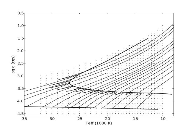
Figure 1.: Location of the BSTAR06 grid models (dots) in the ($T_{\rm eff}$, log $g$)-plane, compared to standard evolutionary models without taking into account rotation and a stellar wind (Pamyatnykh 1999), starting at the right at an intial stellar mass of 4 M_⊙, until 40 M_⊙ at the left. The ZAMS and TAMS are indicated by thick solid lines.

4.2. Diagnostic Lines and their Isocontours of Equivalenth Width

Figure 2.: Isocontours in the ($T_{\rm eff}$, log $g$) plane for several diagnostic lines. Isocontours shown are for weak winds only. Left panel: Si II 4128 (top), Si III 4552 (middle) and Si IV 4116 (bottom). Right panel: He I 4471 (top), He II 4541 (middle) and H$\gamma$ (bottom).

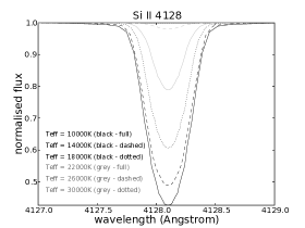
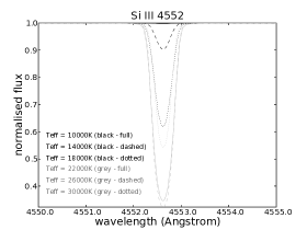
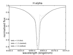
Figure 3.: A simplified, but representative, picture of the effects of $T_{\rm eff}$ on the Si II, III and IV lines (left panels) and the wind properties log $Q$, $\beta$ and $v_{\infty}$ on the H$\alpha$ profile (right panels).

Figure 4.: A simplified, but representative, picture of the influence of the gravity on the wings of H$\gamma$ (left panel: top), of the microturbulent velocity on Si II 4128 (left panel: bottom) and the effect of changing the He and Si abundance (right panels).

Fig.2 shows the isocontours for the equivalent width (EW) of some selected lines. They are based on the complete model grid and represent the dependence of each line on both the effective temperature and the gravity.

Si lines have been chosen because of their strong dependence on temperature. When Si II, Si III and Si IV are considered in parallel, they unambigously define the effective temperature. This is demonstrated in the left panels of Fig.2, by the isocontours for a representative Si line for each of the three ionisation stages: Si II 4128, Si III 4552 and Si IV 4116. Increasing the temperature in the lower temperature region results in an opposite effect regarding the EW of Si II and Si III. Whereas, in the higher temperature region, a similar effect can be observed between Si III and Si IV. This behaviour is demonstrated directly in the line profiles shown in the left panels of Fig.3.

The same is true for He. In the low temperature region, where He I becomes insensitive to gravity, it is the most sensitive diagnostics for changes in the effective temperature (note the almost vertical isocontour). At higher temperatures, where He I looses its diagnostic sensitivity with respect to $T_{\rm eff}$, He II takes over (see Fig.2 - right panel - top and middle). In these regions He I remains useful, but now as a good gravity indicator (note the almost horizontal isocontours). In this way, He I will provide us with a second check for the derived $T_{\rm eff}$ and log $g$ values, but, most important, will allow to derive the He-abundance (from the absolute strength of the lines, see below).

Isocontours of H$\gamma$ (Fig.2 - lower right panel) show that it is equally dependent on $T_{\rm eff}$ and log $g$. Since we can fix $T_{\rm eff}$ already from the Si lines, we can easily determine the gravity by fitting its wings, since these are most affected by even small changes in surface gravity (see Fig.4). Thus, H$\gamma$ is our main gravity indicator.

To obtain the best possible information about the wind properties, we need a line which is sufficiently affected by changes in the wind parameters. The best suited line is H$\alpha$, which is formed in the outer photosphere and lower/intermediate wind. In the right panels of Fig.3, we show the influence of the wind strength parameter log $Q$, the velocity-field exponent $\beta$ and the terminal wind velocity v_∞ on the shape of the resulting (P Cygni) profile.

Of course, this is just the easy picture. There are more things which influence the line profiles, in particular microturbulent velocity v_micro and abundance (He and Si). Their effects are shown in Fig.4, and we will note here only that both quantities have to be derived in parallel, by a rather complex procedure, which nevertheless can be automatized as well.

For reason of brevity, we have restricted ourselves to these figures, because they show the sensitivity to the most fundamental parameters of the star. More could have been drawn, such as the influence of the rotational velocity and the macroturbulent velocity v_macro, which enter the (synthetic) profiles by simple convolutions.

5. Discussion

We have computed a dense grid of NLTE atmosphere models with and without winds covering all spectral types B. The computations were performed continuously during a period of seven months on a dedicated Linux cluster with 20 CPUs (3800 MHz processors with 4 Gb RAM memory and 8 Gb Swap memory). Whenever available these 20 CPUs were extended with 40 extra CPUs (among which 8 more of 3800MHz and 32 of 3400MHz).

In order to avoid unnecessary repetition of the computation of such a huge grid, we will offer BSTAR06 to the community for further research in the near future.

By translating the different effects of the individual parameters on the selected line profiles into code, one can finally perform an automated line profile fitting procedure. This process is currently in its phase of development. Once the automated tool does exist, we will be able to analyse B type stars in a fast and effective way, which hopefully leads to a better understanding of this hot star regime. In particular, the interpretation of the COROT grid should lead to a much better calibration of hot stars across the whole B type spectral range.

Acknowledgments.

We thank Alex de Koter and Rohied Mokiem very heartily for many fruitful discussions and their very useful suggestions for the construction of the model grid. We are also very grateful to Erik Broeders who helped a lot with the technical aspects of the grid calculations.

=======================================

Discussion

Maíz Apellániz: For this grid, will you release the full SEDs or just the line profiles?

Lefever: Only the H, He and Si profiles will be released. More line profiles can easily be added using the calculated model structure, if individual users would require this.

Maíz Apellániz: Once you remove systematic uncertainties, is it possible to measure B-star temperatures with optical-NIR photometry?

Lefever: As far as I know, this is only true for main-sequence stars (not for giants or supergiants). However, this is still based on LTE models, whereas we want to include also the NLTE effects occurring in these massive stars.

Cohen: How do you account for the broadening of the hydrogen lines?

Lefever: Stark broadening is included to correctly treat the broadening of the hydrogen lines.

Adelman: How do these models compare with the recent TLUSTY O and B model grid?

Lefever: TLUSTY is a plane-parallel code, whereas the FASTWIND models assume spherical symmetry. TLUSTY does not include any wind, whereas this is a prerequisite to deal with supergiants.

Adelman: I agree with Dr. Maíz Apellániz that one can get good effective temperatures and surface gravity results for main-sequence band mid- to late-B stars. The use of NLTE model atmospheres is necessary when NLTE effects influence the continuum.

Sterken: Sure, but this work deals with massive stars way above the main sequence.

=======================================

References

- Asplund et al. (2005) Asplund, M., Grevesse, N., & Sauval, A. J. 2005, ASP Conf. Ser. 336: Cosmic Abundances as Records of Stellar Evolution and Nucleosynthesis, 336, 25
- Herrero et al. (2002) Herrero, A., Puls, J., & Najarro, F. 2002, A&A, 396, 949
- Kudritzki & Puls (2000) Kudritzki, R.-P., & Puls, J. 2000, ARA&A, 38, 613
- Lefever, Puls, & Aerts (2006) Lefever, K., Puls, J., & Aerts, C. 2006, submitted to A&A
- Mokiem et al. (2005) Mokiem, M. R., de Koter, A., Puls, J. et al. 2005, A&A, 441, 711
- Pamyatnykh (1999) Pamyatnykh, A. A. 1999, Acta Astronomica, 49, 119
- Puls et al. (1996) Puls, J., Kudritzki, R.-P.; Herrero, A. et al. 1996, A&A, 305, 171
- Puls et al. (2005) Puls, J., Urbaneja, M.A., Venero, R., et al. 2005, A&A, 435, 669
- Santolaya-Rey et al. (1997) Santolaya-Rey, A. E., Puls, J., & Herrero, A. 1997, A&A, 323, 488
=======================================