The Impact of Baryonic Cooling on Giant Arc Abundances

Abstract

Using ray tracing for simple analytic profiles, we demonstrate that the lensing cross section for producing giant arcs has distinct contributions due to arcs formed through image distortion only, and arcs form from the merging of two or three images. We investigate the dependence of each of these contributions on halo ellipticity and on the slope of the density profile, and demonstrate that at fixed Einstein radius, the lensing cross section increases as the halo profile becomes steeper. We then compare simulations with and without baryonic cooling of the same cluster for a sample of six clusters, and demonstrate that cooling can increase the overall abundance of giant arcs by factors of a few. The net boost to the lensing probability for individual clusters is mass dependent, and can lower the effective low mass limit of lensing clusters. This last effect can potentially increase the number of lensing clusters by an extra $50\%$. While the magnitude of these effects may be overestimated due to the well known overcooling problem in simulations, it is evident that baryonic cooling has a non-negligible impact on the expected abundance of giant arcs, and hence cosmological constraints from giant arc abundances may be subject to large systematic errors.

1. Introduction

Soon after the discovery of giant arcs (Lynds & Petrosian, 1986; Soucail et al., 1987) and their subsequent interpretation as gravitational lensing events (Paczynski, 1987), Grossman & Narayan (1988) realized that the statistics of these relatively rare events can be used as a cosmological probe. This idea was greatly expanded by Miralda-Escude (1993a) and Wu & Hammer (1993) who used arc statistics to constrain the mass distribution of clusters and the high redshift galaxy population (Miralda-Escude, 1993b; Bezecourt et al., 1998). Attempts to derive cosmological parameters from arc abundances soon followed, and concluded that giant arc abundances had a relatively mild cosmological dependence (Wu & Mao, 1996).

These early studies used simple analytical models of cluster mass distributions, which turn out to severely under-predict lensing probabilities relative to clusters in numerical simulations (Bartelmann & Weiss, 1994; Bartelmann et al., 1995). Nevertheless, it seemed reasonable to expect that the scaling of arc abundances with cosmology should be broadly consistent with predictions from analytic prescriptions, so it was surprising when the first numerical study to investigate arc abundances in various cosmologies (Bartelmann et al., 1998) found not only that there were order of magnitude differences in the predictions from different cosmologies, but also that the abundance of giant arcs expected in the now-standard $\Lambda\mbox{CDM}$ cosmology is an order of magnitude lower than the observed abundance (Le Fevre et al., 1994).

The claimed sensitivity of giant arc abundances to cosmology and the strong inconsistency between theory and observations found by Bartelmann et al. (1998) generated an explosion of both theoretical and observational studies. On the observational front, new arc samples with more clearly defined selection functions became available (Luppino et al., 1999; Zaritsky & Gonzalez, 2003; Gladders et al., 2003). At the same time, the cosmological community mounted an extensive theoretical effort to search for possible systematics and/or theoretical uncertainties in order to determine whether the disagreement was real.

The theoretical program has revealed that the problem of giant arc statistics is extremely rich, with predictions being sensitive to details of both background galaxies and cluster properties. Concerning sources, many models for giant arc abundances have assumed circular sources, but source ellipticity can significantly boost the number of giant arcs in the sky Bartelmann et al. (1995); Keeton (2001). Assumptions about the distribution of source radii appear to be important (Miralda-Escude, 1993b; Oguri, 2002; Ho & White, 2005). The redshift distribution of sources plays a significant role (Wambsganss et al., 2004; Dalal et al., 2004) and in fact contributes much of the theoretical uncertainty in modern predictions (Hennawi et al., 2005).

There are also several systematics associated with the lens population. For instance, while many studies have assumed spherically symmetric mass distributions (e.g., Hattori et al., 1997; Hamana & Futamase, 1997; Molikawa et al., 1999; Cooray, 1999a, b; Williams et al., 1999), many others have pointed out that halo ellipticity significantly increases giant arc abundances (e.g., Grossman & Narayan, 1988; Bartelmann et al., 1995; Oguri, 2002; Meneghetti et al., 2003b). Moreover, halo triaxiality can give rise to order of magnitude variations in the lensing probability of a given cluster with viewing angle (Oguri et al., 2003; Dalal et al., 2004), and therefore must be treated properly in arc abundance predictions. Lensing probabilities for individual clusters appear to be significantly enhanced during mergers (e.g., Torri et al., 2004; Meneghetti et al., 2005b; Fedeli et al., 2006), though such episodes appear to be rare and transient enough that the overall lens populations is not significantly biased towards a cluster merging population (Hennawi et al., 2005).

One final related trend, noted in both analytical and numerical works, is that lensing probabilities are very sensitive to the radial density profiles of lensing clusters (e.g., Miralda-Escude, 1993a; Hattori et al., 1997; Oguri et al., 2001; Meneghetti et al., 2005a; Hennawi et al., 2005). Consequently, clear predictions for the distribution of cluster density profiles must be in place for arc abundance predictions to become robust.

Systematics that do not seem to have significant effects on lensing probabilities have also been identified. For instance, studies in which a central galaxy is “painted” on the center of simulated clusters suggest that this additional mass component has minimal impact on the expected giant arc abundance (Molikawa & Hattori, 2001; Meneghetti et al., 2003a; Dalal et al., 2004). Likewise, the presence of substructures and/or galaxies in the cluster also seems to have a negligible effect on lensing probabilities (Grossman & Narayan, 1988; Flores et al., 2000; Meneghetti et al., 2000; Hennawi et al., 2005). Line of sight projection effects (Wambsganss et al., 2005) also appear to be unimportant (Hennawi et al., 2005).

At present, there seems to be general agreement between theory and observations (Dalal et al., 2004; Hennawi et al., 2005; Horesh et al., 2005), although the situation is not completely clear (Li et al., 2005). The new agreement arises from the coherent contributions of various effects, with no single systematic explaining the order of magnitude effects observed by Bartelmann et al. (1998). Recent analytical (Kaufmann & Straumann, 2000; Bartelmann et al., 2003) and numerical (Meneghetti et al., 2005a) studies suggest that variations in the arc abundance between different cosmologies are factors of a few rather than an order of magnitude, further relaxing any real tension between theory and observations. What seems clear at this time is that arc abundances are closer to old cosmology than to precision cosmology: agreement is to be understood at the factor of two level, even if current observations did not suffer from small number statistics.

Given the complexity of the problem, it is important to consider whether there are any additional systematic effects that alter theoretical predictions. The goal of this paper is to study one such possibility: the impact of baryonic cooling on cluster mass profiles. Numerical simulations that include cooling have shown that once baryons have cooled and sunk to the center of the halo to form the cluster’s central galaxy, the dark matter halo itself contracts in response to the increased central density (Blumenthal et al., 1986; Kochanek & White, 2001; Gnedin et al., 2004; Sellwood & McGaugh, 2005). The effects of this contraction are significant, and include a steepening of the inner regions of the halo profile, a boost to the mass enclosed within a fixed radius $r$, and an increase of the degree of spherical symmetry of the mass distribution (Kazantzidis et al., 2004). Since arc abundances are known to be sensitive to cluster density profiles we expect that baryonic cooling may significantly affect the predictions. Indeed, recent work by Puchwein et al. (2005) has shown that baryonic cooling enhances the lensing probability of very massive clusters ($M\gtrsim 10^{15}\ \mathrm{M}_{\odot}$) by a factor of $\sim$2–4. Puchwein et al. (2005) did not consider, however, the effect of baryonic cooling on smaller clusters, which is particularly significant given that the median mass of the cluster lens sample (see Hennawi et al., 2005) is well below that considered in Puchwein et al. (2005).

In this work, we extend the analysis of the impact of baryonic cooling on arc statistics to clusters of considerably smaller masses. In particular, we demonstrate that baryonic cooling affects lensing probabilities for low mass clusters more than for high mass clusters, both because low mass clusters have a larger cooled mass fraction, and because lensing in low mass clusters is more confined to the central regions that are strongly affected by cooling. We also demonstrate that baryonic cooling has a strong isotropization effect for both the lensing probability of individual cluster as a function of viewing angle, and the spatial distribution of arcs around the cluster center. In order to understand why baryonic cooling can have such significant impact on the lensing cross section, we develop a theoretical framework that allows us to interpret the lensing probability associated with each cluster as a function of the minimum length to width ratio of the arcs considered. We have found that our theoretical framework can be used to better interpret and contextualize results from previous works, providing an intuitive base upon which the sensitivity of arc statistics to various cluster parameters can be deduced in a qualitative fashion.

2. Lensing Cross Sections

Lensing probabilities are usually characterized in terms of cross sections, so for completeness we review the concept of the lensing cross section. Let ${\rm NewA}$ denote the number of giant arcs per unit area in the sky, expressed as,

$${\rm NewA}=\int dz_{s}dz_{l}d\mathbf{p}\ \frac{d{\rm NewA}}{dz_{s}dz_{l}d\mathbf{p}}$$ (1)

where $d{\rm NewA}/dz_{s}dz_{l}d\mathbf{p}$ is the number of giant arcs due to lenses at redshift $z_{l}$, given sources at redshift $z_{s}$ with structure parameters $\mathbf{p}$ (such as radius and ellipticity). Our immediate goal is to compute $d{\rm NewA}/dz_{s}dz_{l}d\mathbf{p}$. Let $\mathbf{x}$ denote a position vector on the source shell at redshift $z_{s}$ behind a cluster at redshift $z_{l}$. If $r(\mathbf{x})$ is the length to width ratio of the image of a source at position $\mathbf{x}$, then the expected number of arcs with a length to width ratio larger than $\ell$ behind this cluster can be written as $d{\rm NewA}(\ell)=dn_{s}\sigma(\ell;\mathbf{p})$. Here $dn_{s}$ is the number density of sources at redshift $z_{s}$ with parameters $d\mathbf{p}$: $dn_{s}=(dn_{s}/d\mathbf{p})(dV/dz_{s})dz_{s}d\mathbf{p}$. Also, $\sigma(\ell;\mathbf{p})$ is the area of the source plane over which the image of the source satisfies $r(\mathbf{x})>\ell$. This area $\sigma(\ell)$ is called the lensing cross section, and is defined as

$$\sigma(\ell)=\int_{r(\mathbf{x})>\ell}d^{2}\mathbf{x}\ w(\mathbf{x};\ell)$$ (2)

where $w(\mathbf{x};\ell)$ is the number of images of a source placed at point $\bf{x}$ with a length to width ratio larger than $\ell$. If we now denote the average lensing cross section of mass $m$ halos as $\langle\sigma|m;z_{s},z_{l},\mathbf{p}\rangle$, it follows that the number of expected arcs is given by

$$\frac{d{\rm NewA}}{dz_{s}dz_{l}d\mathbf{p}} = \frac{dn_{s}(\mathbf{p};z_{s})}{d\mathbf{p}}\frac{dV}{dz_{s}}$$

$$\times\int dm\ \frac{dn_{\rm halos}}{dm}(m,z_{l})\frac{dV}{dz_{l}}\langle\sigma|m;z_{s},z_{l},\mathbf{p}\rangle,$$

where $dn_{\rm halos}/dm$ is the number density of halos of mass $m$ at redshift $z_{l}$. We can see that the lensing signal is fully characterized by the average lensing cross section $\langle\sigma|m;z_{s},z_{l},\mathbf{p}\rangle$ and the halo mass function $dn/dm$.

To summarize, in order to compute the expected number of giant arcs in the universe one needs to know:

• The halo abundance $dn/dm$ as a function of lens redshift $z_{l}$.

• The source abundance $dn_{s}/d\mathbf{p}$ as a function of source redshift $z_{s}$ and structure parameters $\mathbf{p}$.

• The average lensing cross section for halos of mass $m$, as a function of lens and source redshift and source structure parameters.

Given the evident complexity of the problem, studies that analyze the dependence of lensing cross sections on various parameters are particularly important: they help identify aspects of the theory that need to be well characterized to obtain robust predictions for arc abundances. As we shall see, the lensing cross section $\sigma(\ell)$ tends to exhibit some robust qualitative features, so in this paper we devote considerable effort to understanding these general features in order to provide a robust framework in which we can better interpret our numerical results.

3. Lensing Algorithm and Selection Function

The idea behind our code is simple enough: simulation outputs are used to construct three dimensional pixelized density maps of the clusters, which are then projected to create pixelized surface density maps. Using Fast Fourier Transforms, we compute the gravitational potential, angular deflection, and inverse magnification tensor at each grid point in the lens plane. Following Hennawi et al. (2005), we map each lens plane pixel back to the source plane, where we lay down a grid and associate each source plane pixel with all lens plane pixels contained within it. This yields a lookup table that allows us to quickly find which image (lens plane) pixels are lit given a set of lit source pixels. Circular sources are then placed along an additional coarser grid on the source plane, referred to as the placement grid. For each source, we identify its images and measure their lengths and widths. The lensing cross section for arcs above a given length to width ratio is then estimated from the number of placement pixels which generate appropriate arcs, weighted by the area of each placement grid pixel and the number of arcs produced by said source. All of the various parameters relevant for the algorithm (e.g., grid scales, grid extent, number of pixels, etc.) are chosen to ensure that the resulting cross sections are accurate to 10% or better. We note that because our goal is to estimate the relative change in the lensing cross section of a cluster due to baryonic cooling, we do not expect our conclusions to be very sensitive to assumptions about source size and shape. We have therefore opted to make simple assumptions, and leave a detailed analysis of how source properties affect lensing cross sections to future work.

The details of our algorithm are presented in Appendix A, including various procedures to secure a $10\%$ accuracy in the cross section, and several techniques to improve the speed of the algorithm. In this study, we have chosen to focus on tangential arcs only. This is not only because interpretation of the results is simpler when neglecting radial arcs (see Appendix A, and the discussion in the following sections), but also because we expect the observational selection function for tangential arcs to be simpler than that of radial arcs since the former are more prominent and reside further away from a cluster’s central galaxy than their radial counterparts.

4. Analytic Models

We first study the cross section function $\sigma(\ell)$ for a variety of simple analytical models in order to develop a general understanding of its features. This basic framework will be used in section 5 to analyze the cross section function of numerical clusters.

4.1. The Models

We study halos with projected density profiles of the form

$$\kappa=\frac{b}{2}\ \frac{f(q)h(\beta)}{(q^{2}x^{2}+y^{2})^{\beta/2}}$$ (4)

where $q$ is the projected axis ratio, and $b$ corresponds to the Einstein radius of the profile when $q=1$. The function $f(q)$ is defined by demanding that the mass contained within a circle of radius $b$ be independent of the axis ratio $q$. The parameter $\beta$ is the logarithmic slope of the profile, and $h(\beta)$ is defined by setting $h(1)=1$ and demanding that the mass contained within a circle of radius $b$ be independent of $\beta$. The special case $\beta=1$ corresponds to the Singular Isothermal Ellipsoid (SIE), and the spherically symmetric SIE case is called the Singular Isothermal Sphere (SIS). For an SIS, the relation between Einstein radius and velocity dispersion is

$$b=4\pi\left(\frac{\sigma_{v}}{c}\right)^{2}\frac{D_{ls}}{D_{os}}$$ (5)

where $D_{ls}$ and $D_{os}$ are the angular diameter distances between the lens and the source and between the observer and the source, respectively.

In what follows, we consider two sets of models. For the first set, we fix $\beta=1$ (SIE) and then consider Einstein radii corresponding to velocity dispersions $\sigma_{v}/(10^{3}{\,{\rm km\ s}^{-1}})\in\{0.6,0.7,0.8,0.9,1.0\}$. We also take $q\in\{1.0,0.9,0.8,0.7,0.6,0.5,0.4\}$ for a total of 35 models. For the second set, we fix the Einstein radius to that of an SIS with velocity dispersion $\sigma_{v}=10^{3}{\,{\rm km\ s}^{-1}}$, and then consider density slopes $\beta\in\{0.4,0.6,0.8,1.0,1.2,1.4\}$. We use the same set of axis ratios, for a total of 35 additional models. In all cases we assume typical lens and source redshifts of $z_{l}=0.3$ and $z_{s}=1.5$.

4.2. $\ell$ Maps and Cross-Sections

Since the lensing cross section $\sigma(\ell)$ is simply the area of the source plane in which source produces arcs with length to widths larger than $\ell$, we begin our analysis by looking at $\ell$ maps for our analytic SIE models.

The $\ell$ map of a cluster is defined as the function $\ell(\mathbf{x})$ on the source plane, where $\ell(\mathbf{x})$ is the maximum length to width ratio among all tangential arcs produced by a source centered on $\bf{x}$. Figure 1 shows the $\ell$ map for an SIE profile with velocity dispersion $\sigma_{v}=10^{3}{\,{\rm km\ s}^{-1}}$ and axis ratio $q=0.8$. The topography of the map for the lens is quite striking. In particular, there is a discontinuity all around the lens’s caustic (shown in the figure as a solid black line). The width of this “ribbon” is approximately $2R$ where $R$ is the radius of the source, indicating that all sources placed within this ribbon touch the caustic, and therefore correspond to sources in which distinct images merge to form a single long arc.

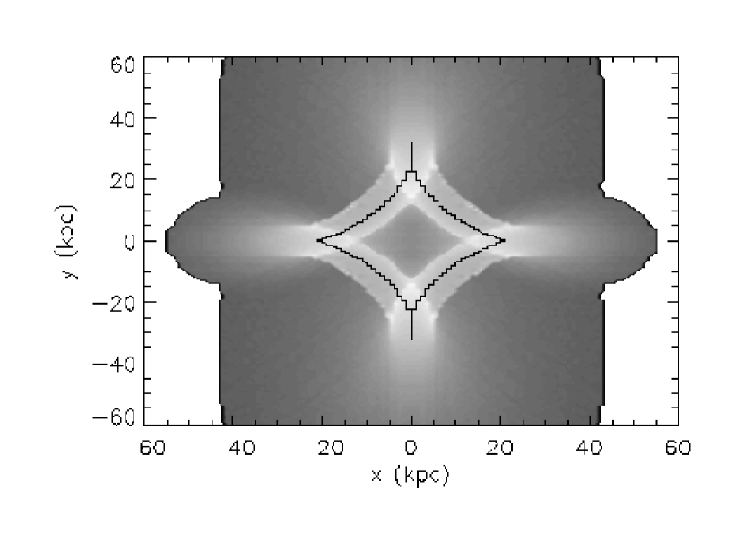
Figure 1.— $\ell$ map for a singular isothermal ellipsoid with $\sigma_{v}=10^{3}{\,{\rm km\ s}^{-1}}$ and $q=0.8$ aligned with the $y$ axis. The map shows the function $\ell(\mathbf{x})$, where $\ell(\mathbf{x})$ is the largest $\ell$ value of all tangential arcs created by a source centered on $\bf{x}$. $\ell$ values are low for dark regions and high for bright regions. The white outside region was not searched for arcs. Finally, the dark, diamond shape solid line is the lens’s caustic. There is a clear discontinuity in the $\ell$ map all around the caustic, corresponding to sources which touch the caustic, and whose longest arcs are therefore formed through the merging of two (fold arcs) or three (cusp arcs) distinct images. The dichotomy between distortion and image merging arcs is also reflected in the shape of the cross section curve $\sigma(\ell)$, as seen Fig. 2.

We therefore introduce a distinction between arcs formed through distortion of a source, and arcs formed through the merging of several images. Moreover, a closer look at the ribbon around the lens’s caustic reveals that there is an additional discontinuity around the lens’s cusps, where not two but three images merge to produce a single arc. To differentiate between these two types of arcs, we shall refer to them as fold arcs and cusp arcs, respectively.

The difference between distortion arcs and image merging arcs is readily apparent in the shape of the cross section function $\sigma(\ell)$, shown in Figure 2 for various SIE profiles at fixed axis ratio $q=0.7$ and for velocity dispersions $\sigma_{v}/(10^{3}{\,{\rm km\ s}^{-1}})=0.6,0.7,0.8,0.9,$ and $1.0$. Each cross section curve exhibits a clear transition, or knee, at some length to width ratio $\ell_{t}$ where it goes from being distortion dominated and roughly power-law, to image merging dominated and roughly exponential in nature. The value of this transition scale $\ell_{t}$ clearly scales with the Einstein radius of the lens, reflecting the fact that sources will be more strongly distorted before touching the caustic for more massive clusters.

Figure 2.— Lensing cross section $\sigma(\ell)$ curves for SIE profiles with axis ratio $q=0.7$. The velocity dispersions of the SIE halos are, from top to bottom, $\sigma_{v}/(10^{3}{\,{\rm km\ s}^{-1}})=1.0,0.9,0.8,0.7,0.6$, and the assumed source radius is $5\ {\,{\rm kpc}}$. The cross section function exhibits a transition between a roughly power law regime at low $\ell$ values, and a roughly exponential regime at high $\ell$. The $\ell$ value at which the transition occurs ($\ell_{t}$) corresponds to the scale at which the lensing cross section switches from being dominated by distortion arcs to being dominated by image merging arcs. The points show the actual results; the solid lines show phenomenological fits discussed in Appendix C.

Since the generic shape of the cross section function $\sigma(\ell)$ — a power law at low $\ell$, and a falling exponential at high $\ell$ — is mainly driven by the difference between distortion arcs and image merging arcs, it is not surprising to learn that this shape is robust to changes in the halo parameters. Our main goal for the rest of this section is to understand how the various features of the lensing cross section function (its amplitude, the position of the transition scale, etc.) depend on the various halo parameters, so that we may better interpret the cross section functions from the numerically simulated clusters.

4.3. The Role of Ellipticity

Figure 3 shows the cross section function $\sigma(\ell)$ of three SIE profiles with velocity dispersion $\sigma_{v}=10^{3}{\,{\rm km\ s}^{-1}}$ and axis ratios $q=0.9$ (diamonds), $q=0.7$ (triangles), and $q=0.5$ (squares). For illustration purposes, we have displaced the $q=0.9$ data upwards by a factor of three, and the $q=0.5$ data downwards by the same amount. The solid lines going through the points represent power law - exponential fits (see Appendix C). It is evident that the transition scale $\ell_{t}$ depends strongly on ellipticity. In particular, the more circular the profile, the larger the value for the transition scale $\ell_{t}$. This reflects the fact that for a circular profile, merging images correspond to rings and typically have large $\ell$ ratios of order $\ell\approx(\pi b)/(2R)$. As the halo becomes more elliptical, arcs straighten out and the images no longer curve around the Einstein radius of the cluster, resulting in a smaller transition scale $\ell_{t}$.

Figure 3.— Lensing cross sections for SIE profiles with a velocity dispersion $\sigma_{v}=10^{3}{\,{\rm km\ s}^{-1}}$ and axis ratios $q=0.5,0.7,0.9$. For illustration purposes, we have displaced the $q=0.9$ data upwards by a factor of three, and the $q=0.5$ data downwards by the same amount. The solid lines are our best fit models. We see that the transition scale $\ell_{t}$ moves towards lower $\ell$ values as the ellipticity of the halo increases. Also shown with dotted lines are all cross section curves with their natural amplitudes. We see that as the halo becomes more elliptical, the amplitude of the image merging contribution to the cross section increases, reflecting the increase in the length of the tangential caustic. The amplitude of the image distortion contribution, however, appears to be roughly independent of halo ellipticity (at fixed Einstein radius).

Also shown in Figure 3 as dotted lines are the un-displaced (i.e., properly normalized) cross section curves for the $q=0.9$ and $q=0.5$ SIE halos. These curves demonstrate that as the halo becomes more elliptical the amplitude of the image merging contribution (high $\ell$) to the cross section increases reflecting the fact that more elliptical halos have longer tangential caustics. More surprising, however, is the fact that the amplitude of the image distortion contribution (low $\ell$) appears to be roughly independent of ellipticity, as evidenced by the fact that all three halos have almost identical cross sections at $\ell\approx 5$. We can understand this result qualitatively as follows: if we take a spherical halo and deform it into an elliptical one, the shear induced by the ellipticity will half the time add to the monopole shear, and half the time subtract from it. Consequently, the net cross section will be roughly unaffected, as illustrated above.

There is one last point of interest that can be garnered from Figure 3: the maxim that elliptical profiles make better lenses is not always correct. More specifically, given a halo of a specified Einstein radius and a $\ell$ ratio of interest, the ellipticity with the highest cross section is that for which the transition scale $\ell_{t}$ is equal to the $\ell$ ratio of interest. For instance, since the cross section quickly falls beyond $\ell_{t}$, at high $\ell$ values ($\ell\gtrsim\pi b/2R$) and fixed Einstein radius only circular profiles are effective lenses.

4.4. The Role of the Density Slope

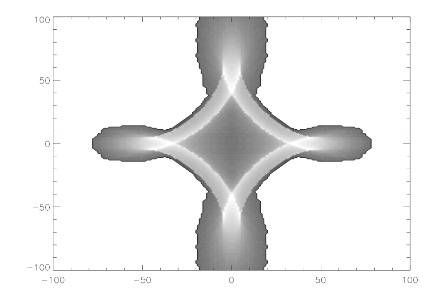
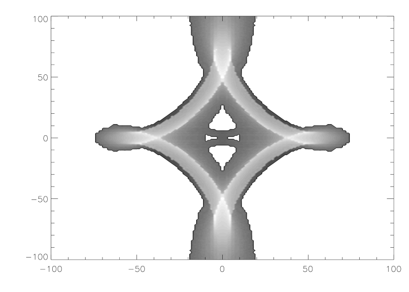
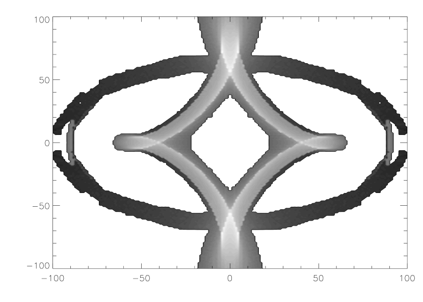
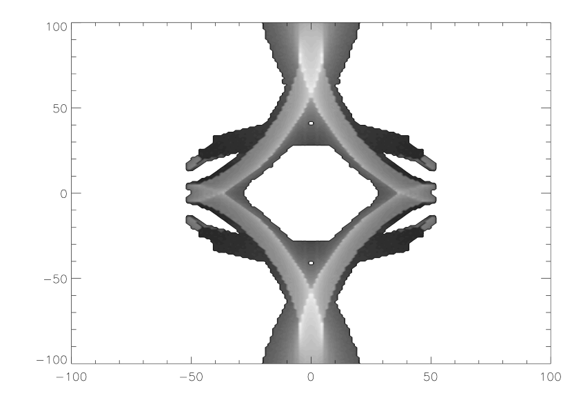
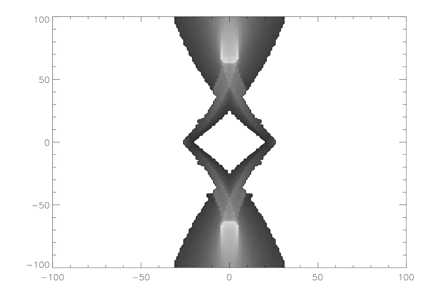
Figure 4.— $\ell$-maps for power-law profiles with axis ratio $q=0.6$, for profile slopes $\beta=1.4$ (top-left), $\beta=1.2$ (top-right), $\beta=1.0$ (middle-left), $\beta=0.8$ (middle-right), $\beta=0.6$ (bottom-left), and $\beta=0.4$ (bottom-right). The long axis of the lens is always along the $y$ axis. The Einstein radius is fixed to that of an SIS with a velocity dispersion $\sigma_{v}=10^{3}\ {\,{\rm km\ s}^{-1}}$. We have used the same gray scale in all maps to allow easy comparison between them. Note that fold arcs and distortion arcs not aligned with the long axis of the lens quickly become smaller (have smaller $\ell$ values) as $\beta$ decreases. For extremely shallow profiles, this reduction in $\ell$ can be so severe that fold arcs may become much smaller than single image arcs along the long axis of the lens, and the fold arc contribution to the cross section becomes unresolved. As a final note, the dark rings seen in some of the maps are due to sources placed along the radial caustic after we filter out the $\ell$ values from the corresponding radial arcs.

To understand how the slope of the density profile affects lensing, we first look at the $\ell$ maps of a series of analytic models. Figure 4 shows the maps for various power-law profiles where we fixed the Einstein radius to that of an SIS with velocity dispersion $\sigma_{v}=10^{3}{\,{\rm km\ s}^{-1}}$ and the axis ratio to $q=0.6$. In order to facilitate comparison between the various maps, we have used the same gray scale in all panels.

We see that the division of arcs into single image, fold, and cusp arcs is generic. What is striking is the strong impact of the profile slope on the length to width ratios of fold, and to a lesser extent, cusp arcs. The “ribbon” around the lens’s caustic decreases monotonically in intensity as $\beta$ decreases, and is even truncated in the case of the $\beta=0.4$ profile. The cusp arcs of the flatter profiles also appear to have smaller length to width ratios than their counterparts in steep profiles, but the difference is less extreme.

A similar pattern is also evident in the image distortion component of the maps, where we see that the length to width ratio of sources not aligned with the long axis of the lens decreases quickly as the profile becomes shallower. We can explain these patterns through a heuristic argument as follows. Consider a small source located off the long axis of the lens. If the halo is highly elliptical, the local curvature of the mass distribution is low and hence the shear induced through ellipticity is low. Likewise, flattening of the profile reduces the shear induced by the mass distribution by making it more uniform, so flat, elliptical profiles are poor lenses if the source is off the long axis of the lens. If a source is along the long axis of the lens, however, the curvature of the mass distribution is high and the resulting images are strongly distorted, even if the profile itself is shallow. Thus, highly elliptical flat profiles will only produce arcs when the sources are placed along the long axis of the lens.

Figure 5.— Cross sections for power law profiles of various slopes $\beta$. The axis ratio is fixed at $q=0.6$, and the Einstein radius is that of an SIS with a velocity dispersion $\sigma_{v}=10^{3}{\,{\rm km\ s}^{-1}}$. The corresponding $\ell$ maps can be seen in Fig. 4. Note that the curves for $\beta\geq 0.8$ are all similar in shape, with the transition scale $\ell_{t}$ decreasing monotonically with $\beta$, reflecting the lower $\ell$ value of fold arcs for shallow profiles. At $\beta=0.6$ the profile becomes so flat that single image arcs along the long axis of the lens can be substantially larger than fold arcs. Consequently, the single image contribution to the cross section “spills over” into the fold arc regime, qualitatively changing the features of the cross section. Further flattening of the profile — the $\beta=0.4$ case — results in such small fold arcs that their contribution to the cross section becomes completely washed out by the single image contribution. The cusp arc contribution, however, becomes prominent, and the generic shape of the cross section is once again similar to that of the steeper $\beta\gtrsim 0.8$ profiles.

Let us now turn our attention to the cross section function $\sigma(\ell)$, shown in Figure 5 for the sample cases from Figure 4. Focus first on the top four curves, corresponding to $\beta=1.4,1.2,1.0,$ and $0.8$. All four of these have the characteristic two-component shape, with the transition scale $\ell_{t}$ decreasing as the profile becomes shallower. This agrees with our expectations: the transition scale $\ell_{t}$ for these curves is roughly the minimum length to width ratio of fold arcs. Since fold arcs become smaller as the profile becomes shallower, the corresponding transition scale decreases.

Turning to the $\beta=0.6$ curve, however, we see that there is no obvious transition. Furthermore, the $\beta=0.4$ curve has a transition that occurs at larger values than the transition for the $\beta=0.8$ case. This behavior may seem puzzling at first, but is easily understood as follows. As $\beta$ decreases from $\beta=0.8$, fold arcs keep getting smaller and smaller, so at some point distortion arcs from sources placed along the long axis of the lens become longer than off-axis fold arcs. In other words, the distortion component of the cross section will “spill over” into the fold arc region, thereby erasing the clear transition observed in the steeper profiles. As $\beta$ is further decreased, fold arcs become negligible, and a new transition becomes evident, but now the transition is between distortion arcs and cusp arcs. This explains why the $\beta=0.4$ transition occurs at higher length to width ratios than the $\beta=0.8$ transition.

There is an additional trend apparent in the cross section functions shown in Figure 5: as the profile gets shallower, the amplitude of the image distortion contribution to the cross section decreases with $\beta$, even though the Einstein radius of the various profiles has been held fixed. This reflects the fact that flat profiles induce little gravitational shear, and are thus not very effective at distorting the images of sources.

5. Simulated Clusters

5.1. The Cosmological Simulations

Next, we analyze high-resolution cosmological simulations of six cluster-size systems in the “concordance” flat $\Lambda$CDM model: $\Omega_{M}=1-\Omega_{\Lambda}=0.3$, $\Omega_{b}=0.04286$, $h=0.7$ and $\sigma_{8}=0.9$, where the Hubble constant is defined as $H_{0}=100\,h{\,{\rm km\ s}^{-1}}{\,{\rm Mpc}}^{-1}$, and $\sigma_{8}$ is the power spectrum normalization on an $8h^{-1}$ Mpc scale. The simulations were done with the Adaptive Refinement Tree (ART) $N$-body$+$gasdynamics code (Kravtsov, 1999; Kravtsov et al., 2002), a Eulerian code that uses adaptive refinement in space and time, and (non-adaptive) refinement in mass (Klypin et al., 2001) to reach the high dynamic range required to resolve cores of halos formed in self-consistent cosmological simulations. The simulations presented here are a subset of the simulated cluster sample presented in Kravtsov et al. (2006) and Nagai et al. (2006), and we refer the reader to these papers for more details. Here we summarize the main parameters of the simulations and list the basic properties of clusters at $z$=0 in Table 1.

High-resolution simulations were run using a 128³ uniform grid and 8 levels of mesh refinement in the computational boxes of $120h^{-1}$ Mpc for CL1-CL3 and $80h^{-1}$ Mpc for CL4-6, which corresponds to the dynamic range of $128\times 2^{8}=32768$ and peak formal resolution of $80/32768\approx 2.44h^{-1}$ kpc, corresponding to the actual resolution of $\approx 2\times 2.44\approx 5h^{-1}$ kpc. Only the region of $\sim$3–10$h^{-1}$ Mpc around the cluster was adaptively refined, while the rest of the volume was followed on a uniform $128^{3}$ grid. The mass resolution corresponds to the effective $512^{3}$ particles in the entire box, or the Nyquist wavelength of $\lambda_{\rm Ny}=0.469h^{-1}$ and $0.312h^{-1}$ comoving Mpc for CL1-3 and CL4-6, respectively, or $0.018h^{-1}$ and $0.006h^{-1}$ Mpc in the physical units at the initial redshift of the simulations. The dark matter particle mass in the region around the cluster was $9.1\times 10^{8}h^{-1}\ \mathrm{M}_{\odot}$ for CL1-3 and $2.7\times 10^{8}h^{-1}\ \mathrm{M}_{\odot}$ for CL4-6, while other regions were simulated with lower mass resolution.

We repeated each cluster simulation with and without radiative cooling and processes of galaxy formation. The first set of “adiabatic” simulations have included only the standard gas dynamics for the baryonic component without gas cooling and star formation. The second set of simulations included gas dynamics and several physical processes critical to various aspects of galaxy formation: star formation, metal enrichment and thermal feedback due to supernovae (type II and type Ia), self-consistent advection of metals, metallicity dependent radiative cooling and UV heating due to cosmological ionizing background (Haardt & Madau, 1996). Throughout this paper, we refer to the adiabatic simulations and simulations with cooling and star formation simply as “adiabatic” and “cooling” run, respectively.

In the cooling run, the cooling and heating rates take into account Compton heating and cooling of plasma, UV heating, and atomic and molecular cooling and are tabulated for the temperature range $10^{2}<T<10^{9}$ K and a grid of metallicities, and UV intensities using the Cloudy code (ver. 96b4, Ferland et al., 1998). The Cloudy cooling and heating rates take into account metallicity of the gas, which is calculated self-consistently in the simulation, so that the local cooling rates depend on the local metallicity of the gas. Star formation in these simulations was done using the observationally-motivated recipe (e.g., Kennicutt, 1998): $\dot{\rho}_{\ast}=\rho_{\rm gas}^{1.5}/t_{\ast}$, with $t_{\ast}=4\times 10^{9}$ yrs. The code also accounts for the stellar feedback on the surrounding gas, including injection of energy and heavy elements (metals) via stellar winds and supernovae and secular mass loss.

Starting from the well-defined cosmological initial conditions, these simulations follow the formation of galaxy clusters and capture the dynamics of dark matter, stars and ICM self-consistently. These simulations can therefore be used to examine the effects of gas cooling and star formation on the density profiles (e.g., Gnedin et al., 2004) and shapes (Kazantzidis et al., 2004) of dark matter halos as well as the roles of substructure present in a realistic cosmological context. Although the magnitude of the effects are likely overestimated in the current simulations due to overcooling problem, the effects of baryon cooling we discuss below are generic.

Table 1Properties of simulated clusters from cooling runs at z=0

Name		$R_{\rm 500c}$	$M_{\rm 500c}^{\rm gas}$	$M_{\rm 500c}^{\rm tot}$
		($h^{-1}$ Mpc)	($10^{13}h^{-1}\ \mathrm{M}_{\odot}$)	($10^{14}h^{-1}\ \mathrm{M}_{\odot}$)
CL1		1.160	8.19	9.08
CL2		0.976	5.17	5.39
CL3		0.711	1.92	2.09
CL4		0.609	1.06	1.31
CL5		0.661	1.38	1.68
CL6		0.624	1.22	1.41

5.2. Surface Density Maps and Ray Tracing

To create the surface density map of a cluster, we begin by nesting $2h^{-1}\ \mathrm{Mpc}$ and $8h^{-1}\ \mathrm{Mpc}$ boxes on the center of the cluster (defined as the position of the most bound dark matter particle in the halo). The boxes have $256$ and $64$ pixels to a side, respectively, and the density at each grid point is computed with a cloud in cell algorithm. The 3D density maps are projected along the region $0\leq r/(1h^{-1}\ \mathrm{Mpc})\leq 1$ and $1\leq r/(1h^{-1}\ \mathrm{Mpc})\leq 4$ for the small and large boxes respectively, and the resulting surface density maps added to produce a 2D surface density map which is $8h^{-1}\ \mathrm{Mpc}$ in extent and reaches a resolution of $7.8h^{-1}\mathrm{kpc}$ in the central regions.

Given the surface density map, we use Fast Fourier Transforms to compute the angular deflection and inverse magnification tensor at each lens plane grid-point. We then select a small region near the center of the lens plane, and refine the lens plane grid using bilinear interpolation. The refined lens plane resolution $r_{l}$ is defined in terms of the source plane resolution $r_{s}$ via $r_{l}=r_{s}/\mbox{max}(\lambda_{\mathrm{R}})$ where $r_{s}$ is the source plane grid resolution and max($\lambda_{\mathrm{R}}$) is the maximum value of the radial eigenvalue $\lambda_{\mathrm{R}}$ over all pixels where $|\lambda_{\mathrm{R}}/\lambda_{\mathrm{T}}|>0.9\ell_{min}$ (i.e., all pixels relevant for lensing). The source plane resolution $r_{s}$ is itself defined via $r_{s}=R/N$ where $R$ is the source radius and $N$ is the number of pixels that “fit” within $R$, for which we take $N=5\sqrt{2}$ as our default value. Finally, once the lens and source plane grids are defined, we link each source plane pixel to every lens plane pixel that maps to it, resulting in a lookup table that can quickly generate the lensed image of any source on the source grid.

5.3. The Impact of Gas Cooling in Lensing Cross Sections

Figure 6.— $\ell$ maps for CL2 in the adiabatic (top) and cooling (bottom) simulations. We have used the same gray scale for both maps to facilitate comparison. The difference between the two maps is dramatic. In particular, adiabatic clusters can produce arcs only for sources located along the major axis of the lens, and these are cusp arcs; fold arcs provide a negligible contribution to the lensing cross section. Cooling clusters, on the other hand, exhibit a much more isotropic arc distribution, and should exhibit prominent fold arcs. These qualitative features are exactly what we would expect given that adiabatic clusters tend to be flat and highly elliptical, whereas cooling clusters are less elliptical and have much steeper profiles in the inner regions of the cluster. These maps are characteristic of all adiabatic and cooling maps we examined in which the central density peak was relatively isolated.

We start by analyzing one of the relaxed clusters with an isolated central density peak to illustrate the general features. Figure 6 shows the $\ell$ maps of the adiabatic and cooling runs of CL2, viewed along a given line of sight. The difference between the two maps is dramatic: the adiabatic cluster is strongly asymmetrical, and arcs can only be produced if sources are placed along the long axis of the lens. The cooling cluster, by contrast, can produce arcs for sources at all azimuthal angles. The cross section for fold arcs is very small in the adiabatic cluster, but prominent in the cooling cluster. These are exactly the trends we would expect based on our analytic models given that adiabatic clusters are flat and highly elliptical, whereas cooling clusters tend to be less elliptical and have much steeper inner density profiles.

Next, we study the effect of gas cooling and star formation on the cross section function $\sigma(\ell)$. Figure 7 shows the average cross section for both the adiabatic and cooling simulations. The impact of baryonic cooling is immediately evident: at $\ell=5$, the boost in the cross section due to cooling is a factor of $\approx 4$. The cooling cluster is capable of forming much larger arcs than the adiabatic cluster because gas cooling enhances the mass in the central regions of the cluster, steepens its density profile, and makes the halo less elliptical. All of these effects make the transition scale $\ell_{t}$ shift to larger values. The net effect is a dramatic increase in the length to width ratio of the arcs that the cluster can produce. Turning this around, we infer that the minimum mass cluster that can produce arcs above some given $\ell$ is smaller with cooling than without. Reducing the effective mass cut may significantly increase the number of lensing clusters, depending on the steepness of the halo mass function. We make an estimate of this effect in section 6.

Figure 7.— The average cross section and its variance among 25 random lines of sight for a massive cluster with a relatively isolated central density peak in cooling (solid line) and adiabatic (dashed line) simulations. Cooling boosts the average cross section by a factor of $\approx 4$ at low $\ell$ and significantly more at higher $\ell$. In addition, it significantly reduces the variance among lines of sight. Finally, note that the cooling cluster is a much more effective lens, capable of producing significantly larger arcs than the adiabatic cluster. This implies that cooling decreases the lower mass cut in lensing-selected clusters.

Also striking in Figure 7 is the difference in the variance in the cross section among different lines of sight: the cooling simulation exhibits considerably smaller variance than the adiabatic one. In the absence of gas cooling, the lensing cross section varies strongly with viewing angle (see also Dalal et al., 2004). This is due to the combined effects of the flatness of the NFW profile and triaxiality of a halo. That is, if the inner density profile is shallow, a small boost to the density due to changes in the viewing angle can dramatically increase the Einstein radius and hence the lensing cross section, resulting in a large dispersion in the cross sections for different lines of sight. In the cooling simulations, by contrast, the Einstein radius and cross section of the lens remain relatively unchanged as we vary the viewing angle. The main reason is that gas cooling steepens the inner density profile of the cluster, making the cross section less sensitive to boosts in the projected mass. The fact that the cooling clusters are less triaxial also contributes to the reduced variance, but is not a dominant effect.

5.4. The Impact of Substructures

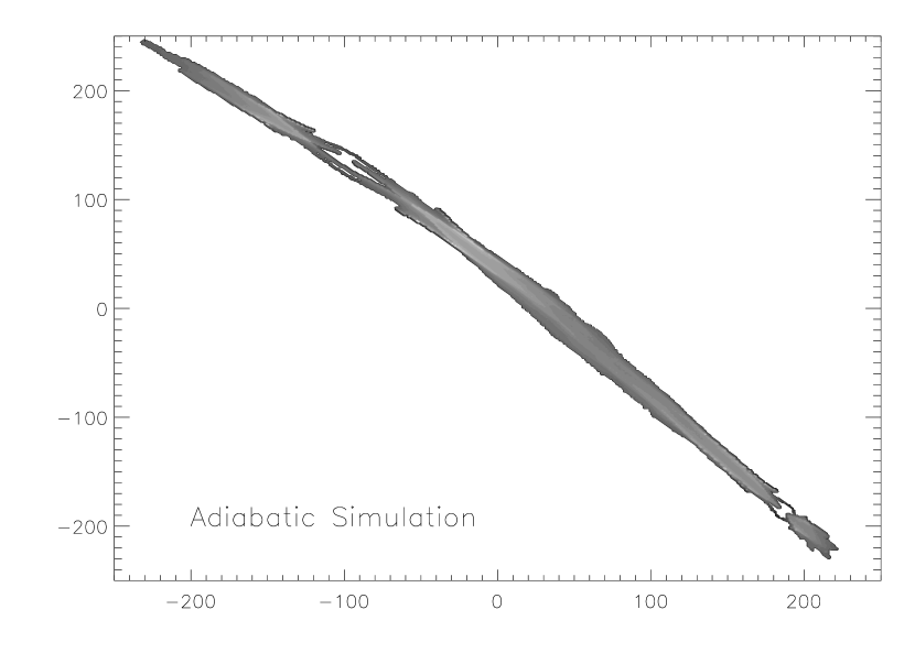
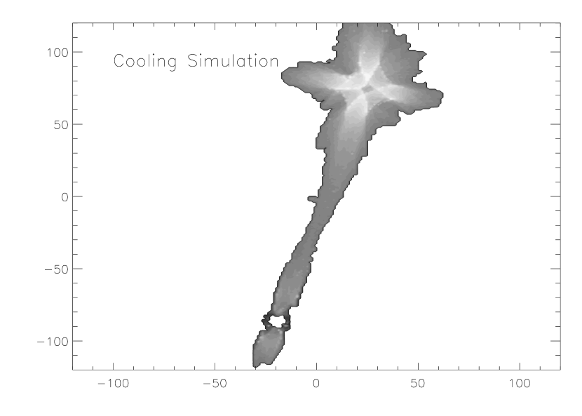
Figure 8.— $\ell$ maps of clusters in which there is substructure near the main density peak. The top panel shows an adiabatic cluster, and the bottom panel shows a cooling cluster (not the same cluster). The basic map topology around the central density peak is largely unaffected by the substructure, though we often found a “bridge” connecting the central density peak with the nearest substructure. This bridge enhances the lensing cross section for moderate length to width ratios, but in general we expect the effect to be modest.

We now examine the effects of substructure on the lensing cross section. Figure 8 shows two typical $\ell$ maps for clusters with substructure, for both adiabatic (top panel) and cooling (bottom panel) simulations. In both cases, substructure leads to the appearance of “bridges” between the central density peak and the most nearby substructure.

It is apparent from the maps, however, that such bridges provide only a modest contribution to the lensing cross section of the largest arcs in both the adiabatic and the cooling clusters, in qualitative agreement with previous estimates of the impact of substructure on the lensing cross section (Meneghetti et al., 2000; Flores et al., 2000; Hennawi et al., 2005).

Figure 9.— The average cross section and its variance for our most massive cluster (CL1). This cluster has substructures present near its central density peak, yet the average cross section function $\sigma(\ell)$ exhibits the same general features seen for the isolated central density peak case examined in Fig. 7. We found this to be true of all the clusters we considered. Thus, the presence of substructures does not appear to significantly affect the impact of baryonic cooling on arc abundances.

Figure 9 shows the average cross section for cluster CL1 over 25 random line of sight projections. Even though the central density peak of CL1 is not isolated, the impact of baryonic cooling on the lensing cross section is strikingly similar to that of CL2, which did have an isolated central density peaks (cf. Fig. 7). In particular, the lensing cross section is still boosted by a factor of $\approx 3$ in the cooling run, and the transition length to width ratio $\ell_{t}$ is again shifted to larger values. We found this to be the case in all of our simulated clusters. We conclude that substructures do not significantly change how baryonic cooling affects arc formation. A complete quantitative characterization of these effect, however, requires a larger cluster sample than what is available to us at this time.

6. The Impact of Baryonic Cooling on Giant Arc Abundance Estimates

As discussed in section 2, estimating the number of giant arcs per unit area in the sky involves characterizing the average lensing cross section $\langle\sigma|m;z_{l},z_{s},\mathbf{p}\rangle$ for halos of mass $m$ as a function of redshift and for a range of source structure parameters (e.g., radius and ellipticity). Since our lens sample is limited to a handful of clusters, we cannot provide a robust estimate of $\langle\sigma|m;z_{l},z_{s},\mathbf{p}\rangle$, even ignoring dependencies on source structure parameters. It is thus evident that extrapolation of our results is necessary, and will involve some guesswork. In light of these difficulties, we have opted to use the simplest possible scaling arguments to estimate the ratio of the number of giant arcs expected in cooling simulations to the number expected in simulations with only adiabatic gas physics.

Our analysis begins by noting that eq. (2) can be written as a product,

$$\frac{dn_{arcs}}{dz_{s}dz_{l}d\mathbf{p}}=g(z_{s},z_{l},\mathbf{p})\ \tau(\ell;z_{s},z_{l},\mathbf{p}),$$ (6)

where

$$g(z_{s},z_{l},\mathbf{p})=\frac{dn_{s}(\mathbf{p};z_{s})}{d\mathbf{p}}\frac{dV}{dz_{s}}\frac{dV}{dz_{l}},$$ (7)

and

$$\tau(\ell;z_{s},z_{l},\mathbf{p})=\int dm\ \frac{dn}{dm}\sigma(\ell|m,z_{s},z_{l},\mathbf{p}).$$ (8)

The quantity $\tau$ is the lensing optical depth, and it contains all of the effects of baryonic cooling on arc abundances. (The function $g(z_{s},z_{l},\mathbf{p})$ does not depend on the internal structure of the lenses.) In particular, the ratio of arcs in the cooling and adiabatic simulations is simply

$$\frac{N_{cool}}{N_{ad}}=\frac{\tau_{cool}}{\tau_{ad}}=\frac{\int dm\ (dn/dm)\ \sigma_{cool}(\ell|m)}{\int dm\ (dn/dm)\ \sigma_{ad}(\ell|m)}.$$ (9)

Our goal is to estimate this ratio. Even this simple scenario requires significant extrapolation from our small sample of clusters, so we again opt for making the argument as simple as possible. We have then

$$\tau_{ad}=\int_{m_{ad}}dm\ \frac{dn}{dm}\sigma_{ad}(\ell|m).$$ (10)

where $m_{ad}$ is the mass cutoff for the adiabatic case and we assume a power law scaling $\sigma_{ad}=C_{ad}m^{\gamma}$. For an SIS lens, $\gamma\approx 1.3$. For a power law halo mass function $dn/dm=Am^{-\alpha}$ we have then

$$\tau_{ad}=\frac{AC_{ad}}{\alpha-\gamma-1}\frac{1}{m_{ad}^{\alpha-\gamma-1}}.$$ (11)

A similar expression holds for $\tau_{cool}$, with $C_{cool}=\lambda C_{ad}$ where $\lambda$ is the net boost to the lensing cross section due to cooling, $\lambda\approx 3$. We see then that

$$\frac{\tau_{cool}}{\tau_{ad}}=\lambda\left(\frac{m_{ad}}{m_{cool}}\right)^{\alpha-\gamma-1}.$$ (12)

The second factor in parenthesis on the right hand side represents the additional boost to the optical depth due to the lowering of the halo mass cutoff. To give a rough estimate for this term, note that the cutoff mass must occur when $\ell\approx\ell_{t}(m)$. We know that $\ell_{t}^{cool}(m)>\ell_{t}^{ad}(m)$, but due to our small cluster sample, we do not know how $\ell_{t}$ scales with mass in either case. However, we can make some progress if we assume a power law scaling between $\ell_{t}$ and $m$, and further assume that cooling only changes the amplitude of this scaling by some fixed factor $f$. In that case, the mass cutoffs $m_{ad}$ and $m_{cool}$ are related via

$$km_{ad}^{\beta}=\ell=fkm_{cool}^{\beta}$$ (13)

where $\beta$ is the slope of the relation $\ell_{t}(m)=km^{\beta}$ for adiabatic clusters. For spherical halos, we know that $\ell_{t}\approx\pi b/2R$, so in general we expect $\ell_{t}\propto b\propto\sigma^{1/2}\propto m^{\gamma}$, and hence $\beta\approx\gamma/2$. Finally, the ratio $f=\ell_{t}^{cool}/\ell_{t}^{ad}\approx 1.5$ in the simulations, which results in

$$\frac{\tau_{cool}}{\tau_{ad}}=\lambda f^{2(\alpha-\gamma-1)/\gamma}.$$ (14)

For $\alpha\approx-3$ as appropriate for clusters, and $\gamma\approx 1.3$ as expected for SIS lenses, we find $(\alpha-\gamma-1)/\beta\approx 1$, meaning the decrease in the halo mass cut due to cooling can further enhance the number of arcs in the sky by about $50\%$. This is smaller than the net increase due to the boost in cross section, but still far from negligible. Moreover, for extremely large arcs, the corresponding mass scale will be larger and hence the mass function will be steeper, thereby enhancing the importance of the change in the mass cutoff scale due to baryonic cooling.

7. Discussion and Comparison With Previous Work

Perhaps the most obvious point of comparison for our work is the work of Puchwein et al. (2005), who studied the impact of baryonic cooling on very massive ($M\gtrsim 10^{15}\ \mathrm{M}_{\odot}$) clusters. To the extent that our analysis overlap, our results are in agreement and we concur with their conclusions: baryonic cooling boosts the lensing cross section of the most massive clusters by a factor of $\approx 2-4$, and this boost is primarily driven by the steepening of the profile. For smaller mass clusters, this boost can be significantly larger, which can in turn significantly increase the number of arcs systems in the universe depending on the minimum length to width ratio of the arcs considered.

In addition to the work by Puchwein et al. (2005), there have been several other studies that investigated the impact of the presence of the massive central galaxy found at the center of most clusters (Meneghetti et al., 2003b; Dalal et al., 2004; Ho & White, 2005). These studies noted that when a mass model for the central cluster galaxies is tacked on numerically simulated dark matter halos the lensing cross section for the cluster is relatively unchanged. This demonstrates that the halo’s response to the baryonic concentration at the center is critically important, and strongly supports our argument that the enhancement to the lensing cross section is driven by the associated steepening of the halo profile.

Incidentally, we expect that the steepening of the halo profile induced by cooling will have an additional interesting effect which we have thus far ignored: it should increase the sensitivity of lensing cross sections to the assumed source redshift. Wambsganss et al. (2004) used the approximation $\mu\approx|\lambda_{\mathrm{R}}/\lambda_{\mathrm{T}}|\approx\ell$ in estimating the impact of source redshift on lensing cross sections, and demonstrated that a broad redshift distribution enhances the lensing optical depth. Subsequent work (e.g., Dalal et al., 2004; Li et al., 2005) demonstrated that the sensitivity to source redshift was overestimated in Wambsganss et al. (2004) since their approximation $\mu\approx\ell$ is exact only for SIS profiles, with shallower profiles resulting in less sensitivity to the source redshift distribution. Given that baryonic cooling tends to both steepen and circularize the halo mass profile, we expect the cooling clusters to be more sensitive to the assumed redshift distribution.

Another interesting way in which our work can be related to previous studies is to ask whether the general theoretical framework developed here can shed some light on previous results. For instance, we have already seen that the question of the isotropy of the lensing cross section is a strong function of the sharpness of the halo density profile, in agreement with the arguments by Dalal et al. (2004) for flat, dark matter only profiles. Likewise, our theoretical framework can help explain how the lensing cross section scales with mass. At low masses, the arc cross section is dominated by merging arcs, and thus should quickly drop with decreasing mass. Conversely, above the mass cutoff, the lensing cross section should become dominated by distortion arcs and have a much more mild mass dependence. This characteristic behavior of a rapidly rising cross section at low masses transitioning into a flatter regime seems to be at least in qualitative agreement with the cross section mass scaling found by Hennawi et al. (2005).

This same type of reasoning can be used to estimate the dependence of lensing cross section on source radii. For instance, consider first the case in which the minimum length to width ratio of interest $\ell\ll\ell_{t}$ where $\ell_{t}$ is the transition scale for a given cluster and source size. In this limit, the cross section is completely distortion dominated and hence source size independent (see appendix B for details). If $\ell\lesssim\ell_{t}$, increasing $\ell_{t}$ will slightly boost the image merging cross section, so we expect the lensing cross section to increase with increasing source size. Conversely, at $\ell\gtrsim\ell_{t}$, the length to width ratio of a source at a fixed distance $d<R$ from the caustic will decrease with increasing source radius due since the source then extending out to regions of lower eigenvalue ratio. This implies that the contour of fixed $\ell$ moves closer to the caustic, and hence the lensing cross section will decrease with increasing source radius.

Based on these arguments, we expect the scaling of the lensing cross section $\sigma(\ell)$ with source radius to be quite complicated. This brings up the question of why should we only consider arcs as a function of their length to width ratio? While early works (e.g., Grossman & Narayan, 1988; Miralda-Escude, 1993a) considered arc abundances as a function of arc length, width, and length to width ratio, this is no longer the case. We expect that the move towards considering only length to width ratios came from the naive expectation that the corresponding cross section would be source radius independent (e.g. Wu & Hammer, 1993). Such a result would imply that arc abundances could be predicted without detailed knowledge of the radius distribution of high redshift galaxies, an observationally challenging problem. Unfortunately, $\sigma(\ell)$ does depend on source radii, so the advantage of considering $\sigma(\ell)$ only is considerably lessened. Rather, given that the source radius dependence of $\sigma(L)$ and $\sigma(\ell)$ are necessarily different, it may be possible to use the abundance of giant arcs as a function of length, width, and length to width ratio simultaneously in order to remove source radii dependences on the predictions. Alternatively, it may be the case that giant arc abundances are better suited to provide constraints on the properties of high redshift galaxies (e.g., Bezecourt et al., 1998). We shall not attempt to resolve this question here.

Figure 10.— The lensing cross section for an SIE profile with axis ratio $q=0.8$ is shown above with diamonds. Also shown as triangles is our estimate for the distortion contribution to the lensing cross section obtained from our best fit model to the data (see Appendix C). The solid line is obtained using the semi-analytic prescription of Fedeli et al. (2006), while the dashed line is the source plane area over which the eigenvalue ratio satisfies $|\lambda_{\mathrm{R}}/\lambda_{\mathrm{T}}|>\ell$. Finally, the dotted line is the result from the semi-analytic prescription of Fedeli et al. (2006) after subtracting the amplitude at the transition scale $\ell_{t}$ as determined by our best fit. As expected, the resulting cross section is in excellent agreement with our best fit estimate of the distortion contribution to the lensing cross section.

The general distinction between distortion and image merging arcs we have introduced also has repercussions for semi-analytic calculations of lensing cross sections. In particular, Fedeli et al. (2006) argued that one may obtain accurate cross sections using a simple method in which the eigenvalue ratio of the inverse magnification tensor is mapped onto the source plane, and then convolved with the appropriate top hat filter for the source under consideration. Since such an algorithm explicitly ignores the possibility of image merging, it is evident that it will underestimate lensing cross sections whenever image merging arcs provide a non-negligible contribution to the total lensing cross section, as shown in Figure 10. Moreover, at fixed length to width ratio the underestimate will become less severe as halo mass increases, an expectation that is fully consistent with the data shown in Fedeli et al. (2006). Note that for the massive clusters considered in Fedeli et al. (2006), we do indeed expect excellent agreement between the semi-analytic estimates and the true lensing cross section.

As a final application of our results, we consider now the multiplicity ratio, the number of clusters with multiple arcs over the number of clusters hosting a single arc. This ratio was first introduced by Gladders et al. (2003) to argue that there must be a population of super lenses: clusters of ordinary mass that for some unknown reason, most likely projection effects, have extraordinarily large cross sections relative to other clusters of comparable mass. This raises the interesting question of how does baryonic cooling affect the multiplicity ratio for a fixed cosmology.

We estimate the impact of baryonic cooling on the multiplicity ratio as follows: the probability $P(2^{+}|1^{+})$ that a cluster with at least one arc host two or more arcs is given by

$$P(2^{+}|1^{+})=\int d\mu P(2^{+}|\mu)P(\mu|1^{+})$$ (15)

where $P(2^{+}|\mu)$ is the probability of observing more than one arc in a halo where the expected number of arcs is $\mu$. $P(\mu|1^{+})$ is the probability that a halo hosting at least one arc has an expectation number of arcs $\mu$. By Bayes’s theorem,

$$P(\mu|1^{+})=\frac{P(1^{+}|\mu)P(\mu)}{P(1^{+})}$$ (16)

and the probability that a halo host at least one arc is

$$P(1^{+})=\int d\mu\ P(1^{+}|\mu)P(\mu).$$ (17)

Putting it all together we find

$$P(2^{+}|1^{+})=\frac{\int d\mu\ (P(2^{+}|\mu)P(1^{+}|\mu)P(\mu)}{\int d\mu\ P(1^{+}|\mu)P(\mu)}.$$ (18)

To compute the multiplicity ratio, we assume Poisson statistics for $P(N|\mu)$, the probability of a halo hosting $N$ arcs given its expectation value $\mu$. For $P(\mu)$ we use the fact that for a halo of mass $m$, $\mu\propto\sigma\propto m^{\gamma}$, so that $P(\mu)\propto\mu^{-\alpha+\gamma-1}$ where $\alpha$ is the slope of the halo mass function at the lensing scale. Finally, the integrals of the above expression are truncated at a lower limit $\mu_{0}$ where we naively expect $0.1\lesssim\mu_{0}\lesssim 1$. Assuming $\mu_{0}$ is the expected number of giant arcs due to clusters at the cutoff mass $m_{ad}$ or $m_{cool}$, we obtain

$$\frac{(\mu_{0})_{cool}}{(\mu_{0})_{min}}=\frac{\sigma_{cool}(m_{cool})}{\sigma_{ad}(m_{ad})}\approx\lambda/f^{2}\approx 1.5$$ (19)

where to obtain a numeric value we used $\gamma\approx 1.3$ as appropriate for an SIS. Thus, even though cooling lowers the lensing mass cutoff, it may slightly increase the effective cutoff in $\mu$, and thus slightly enhance the multiplicity ratio. Perhaps more important, however, is to recognize the fact that our above argument shows that the natural expectation value for the multiplicity ratio is in the range $\approx 0.2-0.6$ as can be directly computed from equation 18, and that this ratio should be fairly robust to details of the halo profile and cosmology, as observed by Ho & White (2005).

8. Summary and Conclusions

Using simple analytic halo density profiles, we have investigated how lensing cross sections depend on various halo parameters. In particular, we found that the lensing cross section has three distinct contributions corresponding to arcs formed through image distortion only, merging of two images, and merging of three images. Moreover, $\sigma(\ell)$ exhibits a knee at the scale which the cross section goes from being distortion dominated to image merging dominated, and the latter component falls exponentially fast with increasing length to width ratio.

We then proceeded to investigate how these various contributions to the lensing cross section depend on halo properties. In particular, we found that while the image merging contribution to the cross section increases with increasing halo ellipticity, the distortion contribution remains relatively constant, except for the fact that it gets truncated at a smaller transition scale $\ell_{t}$. In other words, $\ell_{t}$ decreases with increasing ellipticity. We also investigated the impact of the slope of the profile on the lensing cross section, and found that at fixed Einstein radius, steeper profiles result in more effective lenses, and more circular distribution of arcs about the cluster center. We also noted that the ratio of cusp arcs to fold arcs appears to be very sensitive to the slope of the density profile.

Based on these observations, we argued that the probability for finding arcs of a given length to width ratio should quickly rise with mass below some mass threshold $M_{min}$, and that above this mass cut the scaling should become much flatter. We also discussed how the distinction between arcs formed through image merging and arcs formed through distortion leads to a non-trivial dependence of the lensing cross section on the assumed source radius.

We also investigated the impact of baryonic cooling on the lensing cross section, and found that the steepening of the halo density profile in response to the central baryon condensation enhances the lensing cross section at low $\ell$ by about a factor of three, and lowers the mass threshold $M_{min}$ for halos to become effective lenses. The latter effect helps further increase arc abundances by about $50\%$. Moreover, cooling clusters had a significantly larger probability of forming fold arcs than adiabatic clusters, and their lensing cross section was much less dependent upon the line of sight projection axis than adiabatic clusters. Both of these effects are also explained by the steepening of the halo profile brought about by the contraction of the halo in response to the condensation of cooling baryons at the center. Finally, we also argued that substructures did not appear to significantly enhance lensing cross sections, and that the multiplicity ratio, i.e. the number of lenses that exhibit multiple arcs, is only moderately affected by the details of the mass distribution of the lenses.

Given the sensitivity of arc abundances to baryonic processes, it is difficult to see this observable becoming a tool for precision cosmology in the near future. Conversely, as the range of cosmological parameters get narrower from other observations, this same sensitivity can be used to probe cluster properties and/or the properties of high redshift galaxies. Concerning this last possibility, it seems clear that a systematic analysis similar to the one carried here aimed at understanding how various source properties affect lensing cross section would be a fruitful endeavor which we intend to carry out.

Acknowledgments: E.R. would like to thank Scott Dodelson for a careful reading and helpful suggestions throughout the development of this work. This work was supported in part by the Kavli Institute for Cosmological Physics through the grant NSF PHY-0114422. DN is supported by the Sherman Fairchild Postdoctoral Fellowship at Caltech. AVK is supported by the National Science Foundation (NSF) under grants No. AST-0206216 and AST-0239759 and by NASA through grant NAG5-13274. The authors would also like to thank KICP Thunch, where many conversations related to this topic took place.

Appendix A Lensing Algorithm

In this section, we describe the details of our lensing algorithm, including various procedures to secure a 10% accuracy in the cross section and several techniques to improve the speed of the algorithm.

A.1. Source Placement, and Image Identification and Classification

Having defined the lens and source plane grids, we define the placement grid resolution $r_{p}$ via $r_{p}=R/N$ with $N=5$ as our default value, which is fine enough to adequately resolve the source plane region where sources touch the caustic of the lensing cluster. Now, for our most massive systems, the placement grid may easily have $\gtrsim 2000$ pixels per side with $\lesssim 1\%$ of these pixels producing giant arcs. We therefore seek an efficient algorithm for source placement and image processing.

We proceed as follows. We begin by first placing sources on all grid pixels that map onto a region where $\lambda_{\mathrm{R}}/\lambda_{\mathrm{T}}>0.9\ell_{min}$ and iteratively place sources along the edges of the above region until the placement of additional source do not result in new arcs. We record the position, length, and width of every image generated, as well as the corresponding source position.

The images of an individual sources are processed as follows. First, a list of all lit (not necessarily contiguous) image pixels is made. A random pixel is selected, and we move along the $x$ and $y$ axis until we hit the edge of the image, collecting all lit pixels as we go along. For each pixel collected, we then move in the orthogonal direction, and iterate until no new pixels are collected. We also keep track of edge pixels. The output of this procedure is thus a list of each of the disjoint images along with the edges of each of these images. We note that the procedure described above is much more efficient than the simple neighboring pixel search which is typically employed.

Consider now a single arc. To compute the length and width of the arc we first identify the image pixel containing the center of the source (call it $C$), the pixel farthest from it (call it $F_{1}$), and the pixel $F_{2}$ farthest from $F_{1}$. The length of the image is defined to be that of the circular arc defined by the points $F_{1}\,C\,F_{2}$ plus one pixel unit, the latter being a geometrical correction introduced by Puchwein et al. (2005). Finally, we define the width of the image via $\pi LW=4A$ where $A$ is the area of the image, $L$ is its length, and $W$ its width. Our definition is motivated by the fact that for an ellipse, $\pi LW=4A$.

Figure 11.— Effects of ring images on the lensing cross section $\sigma(\ell)$. The triangles and diamonds points show $\sigma(\ell)$ as a function of L/W with and without ring images for an SIS profile with velocity dispersion $\sigma_{v}=10^{3}{\,{\rm km\ s}^{-1}}$ and lens and source redshifts $z_{l}=0.3$ and $z_{s}=1.5$. This shows that failure to treat rings as such can result in biased lensing cross sections of circularly symmetric profiles. The solid line fit is our analytic fit composed of a power-law distortion component (dotted line) plus a constant contribution corresponding to the cross section for forming rings (dashed line). Note that the total cross section with rings consists of the cross section without rings plus a constant contribution corresponding to the cross section for forming rings, $\pi R^{2}$.

A.2. Circular Profiles and Formation of Rings

There is one special case that our algorithm does not treat properly: that of sources that produce full Einstein rings, since for the latter $A\approx 2\pi LW$ where $W$ is the width of the ring. The obvious way to correct for this is to classify images as arcs or rings, but this can be laborious. Instead, we have opted for a statistical approach. The basic idea is simple: assuming rings are formed, the width distribution of the longest arcs in the sample will be bimodal with a large gap of about a factor of two corresponding to the transition between disjoint arcs and rings. We can thus identify rings by searching for this gap, and then identifying all of the wide “arcs” as rings. Operationally, we identify all arcs with lengths and widths larger than some length and width cuts $L_{cut}$ and $W_{cut}$ as rings, where we set $L_{cut}$ to be 80$\%$ of the length of the widest arc and a width cut $W_{cut}$ to be the median width of all arcs with $L<L_{cut}$. Figure 11 shows the effects of rings on the lensing cross section $\sigma(\ell)$. It shows that failing to treat rings properly resulting in an underestimate of the giant arc cross section for high $\ell$ values since rings are being misidentified as relatively small (low $\ell$) arcs. To correct for this, in this work we simply assign to all rings a length to width ratio $\ell=$max$(\ell)$ where max$(\ell)$ is the maximum length to width ratio of all other arcs.

A.3. Selection Function: Choosing Tangential Arcs

Arcs can form in one of two ways: through strong distortion along the tangential direction, or through the merging of different images of a single source. This is true for both tangential and radial arcs. Therefore, the cross section $\sigma(\ell)$ generally consists of four distinct contributions. However, we have chosen to focus on tangential arcs only, since tangential arcs are much more prominent and easily identifiable than radial arcs. Observationally, this has the advantage that the purity and completeness of a tangential arc sample will be higher than that of a radial arc sample. It is therefore important to identify and remove radial arcs when computing the cross section for tangential arcs.

We have chosen to identify radial arcs through a statistical procedure similar to the one used to identify rings. In particular, we exploit the fact that radial arcs tend to be not just magnified along the radial direction, but also demagnified along the tangential direction. In other words, the radial arcs create a distinct population of images branching out from the main population and reaching the low L and low W part of the plane. We therefore tag all arcs with $L<L_{cut}$ and width $W<W_{cut}$ as radial arcs. The cuts are defined through the following algorithm: first we find the median width of all arcs above the minimum length to width cut $\ell_{min}$, which is our first estimate for $W_{cut}$. We then lower $W_{cut}$ in steps of $0.5r_{p}$ where $r_{p}$ is the placement grid resolution until the increase in the number of arcs with $W>W_{cut}$ is less than $5\%$. The length cut $L_{cut}$ is defined as $L_{cut}=W_{cut}\ell_{min}$ where $\ell_{min}$ is the minimum length to width ratio of arcs considered. We found these cuts cleanly separate the tangential and radial branches.

Appendix B Validity of the Small Source Approximation

One of the key steps in our lensing finding algorithm is selecting all source placement grid pixels where the eigenvalue ratio $\lambda_{\mathrm{R}}/\lambda_{\mathrm{T}}$ is larger than 90$\%$ of the minimum length to width ratio considered. This selection is based on the expectation that for infinitely small sources, the eigenvalue ratio $\lambda_{\mathrm{R}}/\lambda_{\mathrm{T}}$ will be precisely the length to width ratio $\ell$ of the resulting image. A natural question that arises then is to what extent is this small source approximation valid.

Figure 12 illustrates the relation between $L/W$ and $\lambda_{\mathrm{R}}/\lambda_{\mathrm{T}}$ for an SIE model with $\sigma_{v}=10^{3}{\,{\rm km\ s}^{-1}}$ and $q=0.8$. Each point in the figure represents a source that does not touch the lens’s caustic, while sources that touch the tangential caustic are shown as diamonds. This shows that the agreement between $\lambda_{\mathrm{R}}/\lambda_{\mathrm{T}}$ and $\ell$ is excellent provided the source in question does not touch the lens’s caustic. This strongly suggests that the generalization of the eigenvalue ratio $\lambda_{\mathrm{R}}/\lambda_{\mathrm{T}}$ estimate for $\ell$ to elliptical sources proposed by Keeton (2001) should be accurate for distortion arcs, as was indeed found by Fedeli et al. (2006).

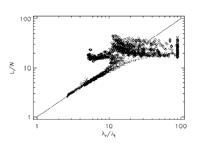
Figure 12.— $\ell$ vs. eigenvalue ratio. The plot is constructed as follows: we begin with an SIE profile with a velocity dispersion $\sigma_{v}=10^{3}{\,{\rm km\ s}^{-1}}$ and an axis ratio $q=0.8$. For each source we place on the source plane, we find its largest arc, and the eigenvalue ratio $\lambda_{\mathrm{R}}/\lambda_{\mathrm{T}}$ at the center of said arc. To keep the $x$-axis small, we set $\lambda_{\mathrm{R}}/\lambda_{\mathrm{T}}=90$ for sources in which $\lambda_{\mathrm{R}}/\lambda_{\mathrm{T}}>90$. Dots represent sources which do not touch the tangential caustic, whereas diamonds correspond to sources that do touch the tangential caustic. It is evident from the figure that the linear approximation $\ell=\lambda_{\mathrm{R}}/\lambda_{\mathrm{T}}$, shown here with the solid line, is a good one even for strongly distorted images, but that the agreement fails if the source touches a caustic. This reflects the fact that the length of these arcs is set by the merging of two images.

Appendix C Fitting Function for Lensing Cross Sections

In this section, we develop an analytic fitting function to the lensing cross sections useful for both analytic and numerical models of galaxy clusters. The idea is based on the realization that at low $\ell$, the lensing cross section curve is dominated by distortion arcs is well fit by a power law, whereas at large $\ell$ ratios, the cross section is dominated by image merging arcs, and is better fit by an exponential fall off. So, the total cross section $\sigma(\ell)$ can be expressed as a sum of these two components:

$$\sigma(\ell)=\sigma_{distortion}(\ell)+\sigma_{merging}(\ell)$$ (C1)

where

$$\sigma_{distortion}(\ell)=\left\{\begin{array}[]{ll}\sigma_{0}\left[\left(\frac{\ell_{0}}{\ell}\right)^{\nu}-\left(\frac{\ell_{0}}{\ell_{d,max}}\right)^{\nu}\right]&\mbox{if}\ \ell<\ell_{d,max},\\ 0&\mbox{if}\ \ell>\ell_{d,max},\end{array}\right.$$ (C2)

and

$$\sigma_{merging}(\ell)=\left\{\begin{array}[]{ll}\sigma_{c}&\mbox{if}\ \ell<\ell_{t},\\ \sigma_{c}\exp\left[-(\ell-\ell_{t})/\ell_{s}\right]&\mbox{if}\ \ell>\ell_{t},\end{array}\right.$$ (C3)

In the above expressions, $\ell_{d,max}$ is the maximum length to width ratio of distortion arcs, and $\ell_{t}$ is the minimum length to width ratio of image merging arcs. The subscript $c$ denotes ‘caustic’, in that image merging sources are those that touch the lens’s caustic.

While $\ell_{d,max}$ tends to be difficult to resolve, we may simply set $\ell_{d,max}=\ell_{t}$ in the above equation. This results in the fitting function:

$$\sigma(\ell)=\left\{\begin{array}[]{ll}\sigma_{0}\left[\left(\frac{\ell_{0}}{\ell}\right)^{\nu}-\left(\frac{\ell_{0}}{\ell_{t}}\right)^{\nu}\right]+\sigma_{c}&\mbox{if}\ \ell\leq\ell_{t}\\ \sigma_{c}\exp\left[-(\ell-\ell_{t})/\ell_{s}\right]&\mbox{if}\ \ell>\ell_{t}\end{array}\right.$$ (C4)

Our ansatz in equation C4 provides an excellent fit to the data whenever the distortion and image merging contributions can be cleanly separated. All fits were done with logarithmic sampling on $\ell$, and assuming an arbitrary $10\%$ error bar at each point. Furthermore, the $\chi^{2}$ surface typically exhibits only one deep minima, implying that degeneracies between the various parameters do not exist when the two components of the lensing cross section are clearly distinct.

Figure 13.— Correlations between the fitting parameters of equation C4. In addition to the correlation between $\ell_{t}$ and $\ell_{s}$ shown by a dashed line, there is an additional correlation between $\ell_{t}$ and the parameter $\ell_{*}$ defined through $\sigma_{0}(\ell_{0}/\ell_{*})^{\nu}=\sigma_{c}$. This latter correlation is shown with the solid line. We have used a least square fitting to define the correlation parameters, and have considered only data in which the cross section function exhibited a clear transition scale, with the added provision that the image merging contribution to the cross section by dominated by fold arcs. Note that the $\ell_{*}$ values have been displaced upwards by five units for illustration purposes. Also shown above are the best fit values obtained from $x$, $y$, and $z$ projections of simulated clusters including cooling and star formations, divided into clusters with a relatively isolated central component (triangles) and clusters with large amounts of substructure near the central density peak (crosses). Note that the best fit relation obtained from our analytic profiles appears to be satisfied by numerical clusters as well.

Note that every parameter has a concrete physical meaning, but these parameters are clearly correlated. For example, we expect the parameters $\ell_{t}$ and $\ell_{s}$ to be correlated, since $\ell_{s}$ is a measure of how quickly the length to width ratio of an arc decreases as the source moves away from the lens’s caustic, and $\ell_{t}$ is the minimum length to width ratio such a source can have while still touching the caustic. Another interesting correlation is between the parameter $\ell_{*}$ and $\ell_{t}$ where $\ell_{*}$ is defined via

$$\sigma_{c}=\sigma_{0}(\ell_{0}/\ell_{*})^{\nu}.$$ (C5)

Thus, $\ell_{*}$ is the length to width ratio at which the image merging cross contribution to the cross section is as large as the image distortion contribution. Figure 13 shows that a clear and tight correlation exists between $\ell_{t}$ and $\ell_{s}$ (dashed line) and between $\ell_{t}$ and $\ell_{*}$ (solid line) for both analytical and simulated cluster data spanning a large range of ellipticities, halo profiles, and Einstein radii. The best fit lines to the $\ell_{t}$–$\ell_{s}$ and $\ell_{t}$–$\ell_{*}$ correlations are given by

$$\ell_{s} = 0.748+0.409\ell_{t},$$ (C6)

$$\ell_{*} = 0.260+0.620\ell_{t}.$$ (C7)

Note that in Figure 13, the $\ell_{*}$ values have been displaced upwards by five units for illustration purposes.

The presence of strong correlations among fit parameters suggests that five parameters are not needed to adequately fit the data; three parameters will suffice, namely $\sigma_{0}$, $\nu,$ and $\ell_{t}$. It turns out that there is a tight correlation between $\nu$ and $\ell_{t}$ as well, further suggesting that lensing cross section curves $\sigma(\ell)$ may, in general, be characterized through only two parameters, an amplitude $\sigma_{0}$ and a transition scale $\ell_{t}$. This is intriguing since the minimal number of parameters to describe a halo are three: an Einstein radius, an ellipticity, and slope profile $\beta$, which raises the interesting question of whether it is possible for two different halos to have the exact same lensing cross section function $\sigma(\ell)$.

References

- Bartelmann et al. (1998) Bartelmann, M., Huss, A., Colberg, J. M., Jenkins, A., & Pearce, F. R. 1998, A&A, 330, 1
- Bartelmann et al. (2003) Bartelmann, M., Meneghetti, M., Perrotta, F., Baccigalupi, C., & Moscardini, L. 2003, A&A, 409, 449
- Bartelmann et al. (1995) Bartelmann, M., Steinmetz, M., & Weiss, A. 1995, A&A, 297, 1
- Bartelmann & Weiss (1994) Bartelmann, M. & Weiss, A. 1994, A&A, 287, 1
- Bezecourt et al. (1998) Bezecourt, J., Pello, R., & Soucail, G. 1998, A&A, 330, 399
- Blumenthal et al. (1986) Blumenthal, G. R., Faber, S. M., Flores, R., & Primack, J. R. 1986, ApJ, 301, 27
- Cooray (1999a) Cooray, A. R. 1999a, ApJ, 524, 504
- Cooray (1999b) —. 1999b, A&A, 341, 653
- Dalal et al. (2004) Dalal, N., Holder, G., & Hennawi, J. F. 2004, ApJ, 609, 50
- Fedeli et al. (2006) Fedeli, C., Meneghetti, M., Bartelmann, M., Dolag, K., & Moscardini, L. 2006, A&A, 447, 419
- Ferland et al. (1998) Ferland, G. J., Korista, K. T., Verner, D. A., Ferguson, J. W., Kingdon, J. B., & Verner, E. M. 1998, PASP, 110, 761
- Flores et al. (2000) Flores, R. A., Maller, A. H., & Primack, J. R. 2000, ApJ, 535, 555
- Gladders et al. (2003) Gladders, M. D., Hoekstra, H., Yee, H. K. C., Hall, P. B., & Barrientos, L. F. 2003, ApJ, 593, 48
- Gnedin et al. (2004) Gnedin, O. Y., Kravtsov, A. V., Klypin, A. A., & Nagai, D. 2004, ApJ, 616, 16
- Grossman & Narayan (1988) Grossman, S. A. & Narayan, R. 1988, ApJ, 324, L37
- Haardt & Madau (1996) Haardt, F. & Madau, P. 1996, ApJ, 461, 20
- Hamana & Futamase (1997) Hamana, T. & Futamase, T. 1997, MNRAS, 286, L7
- Hattori et al. (1997) Hattori, M., Watanabe, K., & Yamashita, K. 1997, A&A, 319, 764
- Hennawi et al. (2005) Hennawi, J. F., Dalal, N., Bode, P., & Ostriker, J. P. 2005, ApJ Submitted. astro-ph/0506171.
- Ho & White (2005) Ho, S. & White, M. 2005, Astroparticle Physics, 24, 257
- Horesh et al. (2005) Horesh, A., Ofek, E. O., Maoz, D., Bartelmann, M., Meneghetti, M., & Rix, H.-W. 2005, ApJ, 633, 768
- Kaufmann & Straumann (2000) Kaufmann, R. & Straumann, N. 2000, Annalen der Physik, 9, 384
- Kazantzidis et al. (2004) Kazantzidis, S., Kravtsov, A. V., Zentner, A. R., Allgood, B., Nagai, D., & Moore, B. 2004, ApJ, 611, L73
- Keeton (2001) Keeton, C. R. 2001, ApJ, 562, 160
- Kennicutt (1998) Kennicutt, R. C. 1998, ApJ, 498, 541
- Klypin et al. (2001) Klypin, A., Kravtsov, A. V., Bullock, J. S., & Primack, J. R. 2001, ApJ, 554, 903
- Kochanek & White (2001) Kochanek, C. S. & White, M. 2001, ApJ, 559, 531
- Kravtsov (1999) Kravtsov, A. V. 1999, PhD thesis, New Mexico State University
- Kravtsov et al. (2002) Kravtsov, A. V., Klypin, A., & Hoffman, Y. 2002, ApJ, 571, 563
- Kravtsov et al. (2006) Kravtsov, A. V., Vikhlinin, A. A., & Nagai, D. 2006, ApJ, in press (astro-ph/0603205)
- Le Fevre et al. (1994) Le Fevre, O., Hammer, F., Angonin, M. C., Gioia, I. M., & Luppino, G. A. 1994, ApJ, 422, L5
- Li et al. (2005) Li, G.-L., Mao, S., Jing, Y. P., Bartelmann, M., Kang, X., & Meneghetti, M. 2005, ApJ, 635, 795
- Luppino et al. (1999) Luppino, G. A., Gioia, I. M., Hammer, F., Le Fèvre, O., & Annis, J. A. 1999, A&AS, 136, 117
- Lynds & Petrosian (1986) Lynds, R. & Petrosian, V. 1986, BAAS, 18, 1014
- Meneghetti et al. (2005a) Meneghetti, M., Bartelmann, M., Dolag, K., Moscardini, L., Perrotta, F., Baccigalupi, C., & Tormen, G. 2005a, A&A, 442, 413
- Meneghetti et al. (2003a) Meneghetti, M., Bartelmann, M., & Moscardini, L. 2003a, MNRAS, 346, 67
- Meneghetti et al. (2003b) —. 2003b, MNRAS, 340, 105
- Meneghetti et al. (2000) Meneghetti, M., Bolzonella, M., Bartelmann, M., Moscardini, L., & Tormen, G. 2000, MNRAS, 314, 338
- Meneghetti et al. (2005b) Meneghetti, M., Jain, B., Bartelmann, M., & Dolag, K. 2005b, MNRAS, 362, 1301
- Miralda-Escude (1993a) Miralda-Escude, J. 1993a, ApJ, 403, 497
- Miralda-Escude (1993b) —. 1993b, ApJ, 403, 509
- Molikawa & Hattori (2001) Molikawa, K. & Hattori, M. 2001, ApJ, 559, 544
- Molikawa et al. (1999) Molikawa, K., Hattori, M., Kneib, J.-P., & Yamashita, K. 1999, A&A, 351, 413
- Nagai et al. (2006) Nagai, D., Vikhlinin, A. A., & Kravtsov, A. V. 2006, ApJ, submitted (astro-ph/0609247)
- Oguri (2002) Oguri, M. 2002, ApJ, 573, 51
- Oguri et al. (2003) Oguri, M., Lee, J., & Suto, Y. 2003, ApJ, 599, 7
- Oguri et al. (2001) Oguri, M., Taruya, A., & Suto, Y. 2001, ApJ, 559, 572
- Paczynski (1987) Paczynski, B. 1987, Nature, 325, 572
- Puchwein et al. (2005) Puchwein, E., Bartelmann, M., Dolag, K., & Meneghetti, M. 2005, A&A, 442, 405
- Sellwood & McGaugh (2005) Sellwood, J. A. & McGaugh, S. S. 2005, ApJ, 634, 70
- Soucail et al. (1987) Soucail, G., Fort, B., Mellier, Y., & Picat, J. P. 1987, A&A, 172, L14
- Torri et al. (2004) Torri, E., Meneghetti, M., Bartelmann, M., Moscardini, L., Rasia, E., & Tormen, G. 2004, MNRAS, 349, 476
- Wambsganss et al. (2004) Wambsganss, J., Bode, P., & Ostriker, J. P. 2004, ApJ, 606, L93
- Wambsganss et al. (2005) —. 2005, ApJ, 635, L1
- Williams et al. (1999) Williams, L. L. R., Navarro, J. F., & Bartelmann, M. 1999, ApJ, 527, 535
- Wu & Hammer (1993) Wu, X.-P. & Hammer, F. 1993, MNRAS, 262, 187
- Wu & Mao (1996) Wu, X.-P. & Mao, S. 1996, ApJ, 463, 404
- Zaritsky & Gonzalez (2003) Zaritsky, D. & Gonzalez, A. H. 2003, ApJ, 584, 691